Sage Journals: Discover world-class research

Abstract

Selection of appropriate operating conditions is an important attribute to pay attention for in electrical discharge machining (EDM) of steel parts. The achievement of EDM process is affected by many input parameters; therefore, the computational relations between the output responses and controllable input parameters must be known. However, the proper selection of these parameters is a complex task and it is generally made with the help of sophisticated numerical models. This study investigates the capacity of Adaptive Nero-Fuzzy Inference System (ANFIS), genetic expression programming (GEP) and artificial neural networks (ANN) in the prediction of EDM performance parameters. The datasets used in modelling study were taken from experimental study. According to the results of estimating the parameters of all models in the comparison in terms of statistical performance is sufficient, but observed that ANFIS model is slightly better than the other models.

1. Introduction

Recently, as a result of advances in technology, the use of a variety of materials with superior properties has become commonplace. Manufacturing of these materials is extremely difficult or impossible via traditional machining process; however, EDM is a mostly used process for manufacturing such parts [1]. In EDM process, material is removed rapidly and repeatedly by spark discharges across the gap between the workpiece and the tool, both of them are immersed in a dielectric. Surface roughness (R_a), material removal rate (MRR), and electrode wear ratio (EWR) are the most important output parameters from the point of efficiency and quality. Many input parameters affect these performance parameters; therefore, the appropriate selection of the input parameters is needed.

Determining the optimum process parameters is important in terms of increasing the surface quality, reducing the processing time, and the tools wear [2]. But metal removal process in EDM has a nonlinear, randomness, and time varying properties [3]. EDM process is requiring much skill or effort but it has a quite complex mechanism and its mechanism is still not exactly understood. The application area of EDM process is limited due to its disadvantages such as lower productivity, a high specific energy consumption, and longer processing time. To create a model that can predict EDM performance by using input parameters with high accuracy is very difficult. However, a quantitative relationship between the performance parameters and controllable input parameters is often needed in EDM. Mathematical models help to know the effects of different process variables on the output performances and enhance the operating performance by applying some of the theoretical outcomes [4]. Therefore, researches are concentrating on the optimization and the process modeling of EDM in order to develop the productivity and finishing capability in last decades. Some regression methods have been applied for modelling the EDM process [5]. Because of the advantages of the artificial intelligence systems, many researchers studied to find the relationships between input and output parameters in EDM process by using soft computing techniques.

Indurkhya and Rajurkar [6] presented an ANN model. MRR and surface roughness estimating capability of different ANN algorithms were investigated by Tsai and Wang [7, 8]. Lin et al. investigated the grey relational analysis based on an orthogonal array and fuzzy-based Taguchi method for optimizing the EDM process [9]. A hybrid ANN and GA methodology to modeling and optimization of EDM were used by Wang et al. [10]. An artificial feed forward NN based on the Levenberg-Marquardt backpropagation technique was developed to estimate the MRR by Panda and Bhoi [11]. For the selection of EDM process parameters, Yilmaz et al. developed a fuzzy logic-based system [12]. Mandal et al. used an ANN and backpropagation algorithm for modelling and optimizing the EDM process [2]. Salman and Kayacan developed a model between EDM inputs and R_a by using GEP [13]. Rao et al. developed a hybrid model using ANN and GA for modelling and optimization of surface roughness (R_a) in EDM [14]. Maji and Pratihar used (ANFIS) to establish input-output relationships of an electrical discharge machining both in forward as well as reverse directions in 2010 [15]. Joshi and Pande reported an intelligent approach for process modelling and optimization of (EDM) [16]. Though many modelling studies for EDM process have been done until now, these models are based on several assumptions and they cannot be generalized to all conditions; therefore, modelling studies will go on in the future.

However, a comprehensive study to compare the performances of GEP, ANN, and ANFIS for modelling of important EDM performances is still missing. The aim of this study is to compare the mostly used soft computing techniques which are ANN, ANFIS, and GEP in prediction accuracy of the EDM process. In this study, soft computing techniques are applied on the outcomes of experimental works. Discharge current, pulse on-time, and pulse off-time were taken as input parameters and surface roughness, electrode wear ratio, and material removal rate are taken as the output parameters. Using the experimental dataset, ANFIS, ANN, and GEP models are developed and then their performances were compared.

2. Experimental Studies

The die sinking EDM machine (Furkan Model M50A) with servo head (constant gap) is used to conduct the experiments. Twelve mm depth blind holes were formed using different parameters. Electrode was copper with 20 mm diameters and dielectric liquid was kerosene. During the experiments, pulse off-time (T_off), pulse on-time (T_on), and discharge currents (I) were taken as variable parameters. Gap voltage, flushing pressure, and polarity were kept constant. Values of these parameters are shown in Table 1. The work material used in this study was DIN 1.2080 tool steel. The dimension of the work material was 60 mm in diameter and 30 mm in height.

Table 1:

Machining conditions in EDM.

	Levels

Variable parameters
Discharge current, I (A)	3, 6, 12.5, 25, 50
Pulse on-time, T_on (μs)	3, 6, 12, 24, 48, 99, 201, 402, 801, 1602
Pulse off-time, T_off (μs)	3, 6, 12, 24, 48, 99, 201
Constant parameters
Dielectric	Kerosene
Gap voltage (volt)	60–80 V
Dielectric flushing pressure	0.1 MPa
Polarity of tool electrode	Positive, +

Machining performances of EDM are influenced be various process parameters and these parameters can be varied in each stage of EDM. Selection of variable and constant input parameters is based on work experience, handbook values, and researchers' reports [17 –19]. General EDM performances parameters are surface roughness, MRR, and EWR except for the electrode material type and dielectric fluid [17].

MRR in EDM is an important factor to estimate the time of finishing the machined part. MRR in EDM process is an important factor because of its vital effect on the industrial economy. MRR is commonly described as material volume per min (mm³/min) and calculated as the removed mass from the workpiece material during the machining by dividing into the machining time and density of workpiece. MRR value is calculated from the following equation:

MRR = \frac{W_{f} - W_{i}}{t \times ρ} = {mm}^{3} / \min,

(1)

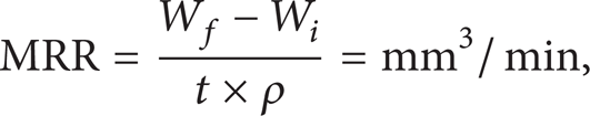
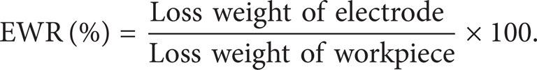
where W_i = initial mass of workpiece material (g), W_f = final mass of workpiece material (g), t = operating time (min), and ρ = density of workpiece (g/mm³). Accuracy of the product size is influenced by electrode wear and therefore much research is being done to minimize electrode wear. Minimum discharge current gives minimum electrode wear but in that case MRR will decrease. Conversely the high current gives a high MRR with high electrode wear. Completely elimination of electrode wear is not possible, but it can be reduced by selecting optimum settings of input parameters. The ratio of loss weight of the electrode to the loss weight of workpiece material is defined as EWR and mostly expressed as a percentage as

EWR (%) = \frac{Loss weight of electrode}{Loss weight of workpiece} \times 100 .

(2)

One of the most important quality parameters of the EDM process is workpiece surface roughness. Average surface roughness (R_a) among the various amplitude parameters is mostly used in EDM process. In this study, in order to measure surface roughness values of machined samples, Mahr stylus instrument (MarSurf XR 20 with GD 25) available was used. Experimental results of three performances and prediction of all models are given at Tables 13 –17.

3. Modelling Study

The artificial intelligence approaches have lately emerged as promising for developing a useful model for the complex systems. The purpose of this study is to present a proficient and incorporated approach to establish a model that can accurately predict the performances of EDM process by correlating the input parameters. Therefore, the well-known soft computing methods such as ANFIS, GEP, and ANN were compared for predicting performances. Thus the precision, efficiency, and quality of EDM process can be improved by choosing the best model.

3.1. Development of Genetic Programming (GP) Models

GP is an artificial intelligence method which has many application areas like engineering, science, and industrial and mechanical models [20 –22]. GP proffers a solution as a result of the evolution of computer programs by using natural selection methods. Genetic programming (GP) was developed by Koza [23]. GP is a propagation of the traditional genetic algorithm (GA). Ferreira invented an evolutionary algorithm called gene expression programming (GEP) to predict mathematical models by using experimental data in 2001 [24]. GEP includes simple linear chromosomes of fixed length like that used in GA and forked forms of various sizes and shapes similar to the parse trees of GP [25].

In this study GeneXproTools 4.0 program was used to develop mathematical models which are used to estimate MRR, EWR, and R_a values. Primarily the chromosomes of a number of individuals are produced fortuitously in the GEP process. Then the chromosomes are stated as expression trees (ETs), evaluated based on a fitness function, and selected by fitness to reproduce with modification by means of genetic operations. The new generation of solutions experiences the same process and the process is repeated until the stop condition is fulfilled. The fittest individual is used as the final solution [26].

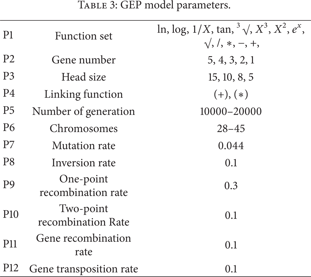
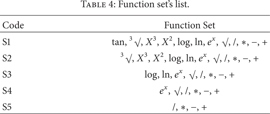
Experimental parameters and their ranges are shown in Table 2, and parameters which are used for construction of GEP models are specified in Table 3. The list of function set is presented in Table 4. The data obtained from experimental study is separated into two parts as training and test sets to find out explicit formulations. The results of GEP models obtained from different combinations are presented in Table 5. Longer computational time was needed for training all of these combinations. Hence a subset of these combinations was chosen to analyse the GEP performance's algorithm for estimating the MRR, EWR, and R_a. The optimal settings obtained from GEP models are shown as bold in Table 5. Consequently, these optimal settings are used for the estimation of all performances.

Table 2:

Input and output parameters of GEP models.

	Code	Variables	Symbol	Range

Input	d0	Discharge current (Ampere)	I	3–50
Input	d1	Pulse on-time (μs)	T _on	3–1602
Input	d2	Pulse off-time (μs)	T _off	3–201
Output 1	F1	Material removal rate (mm³/min)	MRR	3.4–390
Output 2	F2	Electrode wear ratio (%)	EWR	0.01–45
Output 3	F3	Surface roughness (μm)	R _a	1.4–18

Table 3:

GEP model parameters.

P1	Function set	ln, log, 1/X, tan, ³ √, X³, X², e^x, √,/, *, −, +,
P2	Gene number	5, 4, 3, 2, 1
P3	Head size	15, 10, 8, 5
P4	Linking function	(+), (*)
P5	Number of generation	10000–20000
P6	Chromosomes	28–45
P7	Mutation rate	0.044
P8	Inversion rate	0.1
P9	One-point recombination rate	0.3
P10	Two-point recombination Rate	0.1
P11	Gene recombination rate	0.1
P12	Gene transposition rate	0.1

Table 4:

Function set's list.

Code	Function Set

S1	tan, ³ √, X³, X², log, ln, e^x, √,/, *, −, +
S2	³√, X³, X², log, ln, e^x, √,/, *, −, +
S3	log, ln, e^x, √,/, *, −, +
S4	e^x, √,/, *, −, +
S5	/, *, −, +

Table 5:

The results obtained from GEP models.

				MRR			EWR			R _a
				R² error			R² error			R² error
P1	P2	P3	P4	P5	Train	Test	P5	Train	Test	P5	Train	Test

1	2	5	+	12115	0.992	0.986	12169	0.980	0.983	12964	0.966	0.964
S1	2	5	*	18751	0.994	0.979	19907	0.915	0.923	10272	0.993	0.990
S1	3	8	+	18725	0.995	0.987	15916	0.947	0.923	11373	0.993	0.992
S1	3	8	*	17185	0.987	0.961	12170	0.967	0.978	11268	0.968	0.976
S1	4	10	+	18022	0.995	0.995	15130	0.918	0.900	11514	0.977	0.957
S1	4	10	*	14363	0.993	0.990	13788	0.919	0.820	13170	0.992	0.988
S1	5	15	+	14628	0.992	0.992	15273	0.941	0.910	19517	0.990	0.983
S1	5	15	*	18125	0.995	0.988	14868	0.869	0.871	17871	0.991	0.993
S2	2	5	+	17574	0.993	0.989	12716	0.954	0.964	12239	0.992	0.993
S2	2	5	*	18880	0.991	0.990	17180	0.900	0.891	11899	0.992	0.991
S2	3	8	+	17606	0.993	0.991	11404	0.980	0.862	10227	0.984	0.985
S2	3	8	*	18607	0.991	0.889	15687	0.981	0.932	10314	0.991	0.991
S2	4	10	+	13058	0.988	0.987	12108	0.941	0.907	14376	0.989	0.979
S2	4	10	*	18954	0.957	0.955	12564	0.854	0.868	11353	0.984	0.982
S2	5	15	+	14440	0.994	0.991	18056	0.941	0.923	19195	0.991	0.987
S2	5	15	*	12960	0.993	0.979	12577	0.926	0.904	17192	0.903	0.948
S3	2	5	+	14480	0.991	0.985	13080	0.952	0.957	10129	0.987	0.988
S3	2	5	*	14780	0.994	0.994	14465	0.956	0.916	11534	0.992	0.992
S3	3	8	+	14169	0.989	0.985	16631	0.981	0.891	10807	0.992	0.990
S3	3	8	*	13686	0.995	0.992	14565	0.974	0.927	11011	0.971	0.955
S3	4	10	+	17130	0.995	0.989	11764	0.944	0.910	10863	0.983	0.981
S3	4	10	*	18529	0.994	0.864	11405	0.961	0.938	13042	0.991	0.992
S3	5	15	+	11502	0.994	0.994	17243	0.926	0.905	18962	0.981	0.949
S3	5	15	*	11890	0.986	0.975	17553	0.927	0.913	19290	0.993	0.993
S4	2	5	+	12340	0.981	0.981	11981	0.977	0.965	15561	0.991	0.990
S4	2	5	*	13152	0.993	0.992	10536	0.978	0.986	14886	0.985	0.764
S4	3	8	+	12879	0.985	0.982	15429	0.955	0.947	13396	0.973	0.968
S4	3	8	*	15082	0.995	0.978	11563	0.981	0.980	13043	0.992	0.994
S4	4	10	+	18092	0.990	0.987	10491	0.909	0.908	10552	0.993	0.994
S4	4	10	*	19587	0.993	0.992	18350	0.885	0.820	13543	0.982	0.989
S4	5	15	+	12021	0.995	0.993	12543	0.928	0.930	17273	0.991	0.977
S4	5	15	*	12165	0.972	0.992	16252	0.680	0.780	16555	0.990	0.888
S5	2	5	+	19635	0.996	0.995	18978	0.976	0.976	15273	0.979	0.980
S5	2	5	*	12069	0.993	0.994	11267	0.977	0.979	15865	0.900	0.896
S5	3	8	+	14075	0.995	0.989	12766	0.809	0.765	11841	0.815	0.898
S5	3	8	*	18934	0.995	0.993	16346	0.983	0.988	12751	0.951	0.903
S5	4	10	+	17575	0.995	0.987	10901	0.975	0.937	10802	0.987	0.820
S5	4	10	*	15170	0.990	0.995	16341	0.903	0.768	13875	0.948	0.945
S5	5	15	+	12506	0.992	0.965	19621	0.956	0.914	12004	0.973	0.950
S5	4	10	*	11042	0.975	0.963	10924	0.821	0.801	17834	0.977	0.968

In this study three statistical parameters were used for measuring performance of GEP models. They are coefficient of correlation (R²), mean square error (MSE), and mean absolute error (MAE). Table 6 shows the best statistical results obtained from GEP formulation.

Table 6:

Best statistical results obtained from GEP formulation.

Statistical parameters	(MRR)		(EWR)		(R_a)
Statistical parameters	Training	Testing	Training	Testing	Training	Testing

MSE	55.351	162.23	3.5504	3.6266	0.0966	0.2201
MAE	5.4858	8.3515	1.2967	1.2536	0.2361	0.3378
R ²	0.996	0.995	0.983	0.988	0.993	0.994

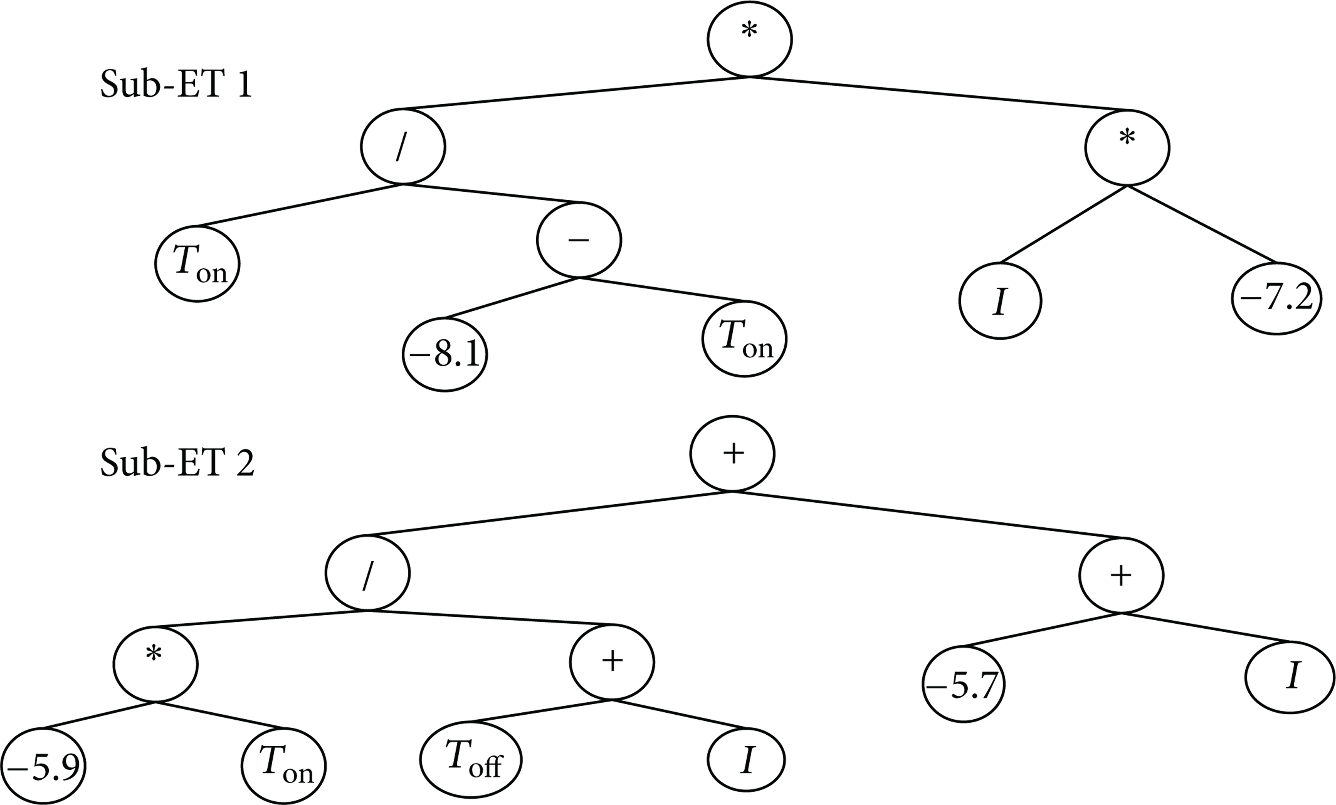
Test and training datasets used for construction of all models are selected randomly. Regarding the MRR, EWR, and R_a formulation, 30 training data and 10 test data were used. The offered GP formulations must be suitable range as remarked in Table 2. The formulations resulting from training values are checked by test values. The GEP modelling results in the expression tree form are presented in Figures 1, 2, and 3 which correspond to the following equations:

\begin{matrix} MRR = \frac{7.2 \times I \times T_{on}}{8.1 + T_{on}} + \frac{- 5.9 \times T_{on}}{T_{off} + I} + I - 5.7, \\ EWR = \frac{- 4.8 \times (I \times T_{on} + T_{on})}{((T_{off} / T_{on}) + I + T_{on})} \times \frac{- 5.1}{T_{on} + ((T_{on}^{2} + T_{off}) / I^{2})} \times 1.93, \\ R_{a} = {(2 \times T_{on} \times I)}^{1 / 4} - T_{on} - 2 \times T_{off} + T_{off} - e^{[- 8.7 - e^{I - T_{off}} - 8.6]} + T_{off} - e^{[I - e^{I + 1.9} + 0.1 + I]} + T_{on} e^{[I - ((T_{on} - I) / (I - 9)) + I + T_{on}]} . \end{matrix}

(3)

Figure 1:

Expression tree for MRR.

Figure 2:

Expression tree for EWR.

Figure 3:

Expression tree for R_a.

3.2. Development of Artificial Neural Networks (ANN) Models

An artificial neural network is a model which runs like a human brain by using many neurons consecutively. The network collects information by a learning process [26]. Complex problems whose analytical or numerical solutions are difficult to be obtained and can be solved by utilizing adaptive learning ability of neural networks [27]. Neural networks are generally classified according to their network topology (i.e., feedback or feedforward) and learning or training algorithms (i.e., supervised or unsupervised). Multilayer perceptron (MLP) which is the most common neural network model is a feedforward neural network with one or more hidden layers [28]. MLP is a supervised type network as it needs a desired output to learn. The main advantage of MLP is that it is easy to use and its capability of approximating arbitrary functions in terms of mapping abilities. The requirement of longer training time and lots of training data (typically three times more training samples than network weights) are the main disadvantages.

Normally, the network consists of an input layer of source neurons, at least one middle layer or hidden layer of computational neurons, and an output layer of computational neurons. A multilayer perceptron with one hidden layers is shown in Figure 4. Each layer in a multilayer neural network has its own specific function. The function of input layer is accepting the input signals from environment and redistributing these signals to each neuron in the hidden layer. The function of output layer is receiving the output signals from the hidden layer and creating the output model of the entire network. Neurons in the hidden layer perceive the features; the weights of the neurons represent the features hidden in the input patterns. These features are then used for determining the output pattern by the output layer.

Figure 4:

Three-layered feed forward neural network topology.

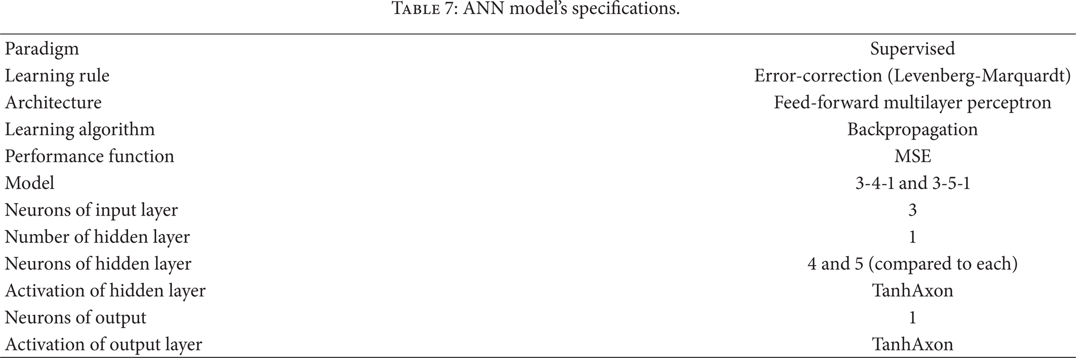
In this study, an ANN model was designed in MATLAB (version 7.0) environment. This developed ANN model's specifications are listed in Table 7. The developed ANN model consists of one input layer, one hidden layer, and one output layer. The inputs to be used in the ANN are the same as the ones in GEP models.

Table 7:

ANN model's specifications.

Paradigm	Supervised
Learning rule	Error-correction (Levenberg-Marquardt)
Architecture	Feed-forward multilayer perceptron
Learning algorithm	Backpropagation
Performance function	MSE
Model	3-4-1 and 3-5-1
Neurons of input layer	3
Number of hidden layer	1
Neurons of hidden layer	4 and 5 (compared to each)
Activation of hidden layer	TanhAxon
Neurons of output	1
Activation of output layer	TanhAxon

Firstly training and test data sets were created, and then the best structure of MLP for this application was developed by training of different types of transfer and output functions for layers and also different numbers of hidden layers and its neurons were developed as well, and at the end, the neural network model was established by comparing the network prediction to validation data (10% of the data). In this study, the neuron numbers in the hidden layer were used as a main parameter to obtain the best ANN structure. Therefore, they were changed until achieving the minimum mean squared error. Regarding the MRR, EWR, and R_a formulation, 30 training, 4 validation, and 6 tests data were used as training and test sets. From this trial and error study, TanhAxon function was found tobe the most compatible one for the hidden layer and output layer in all tested ANN models. TanhAxon squashes the range of each neuron in the layer to between −1 and 1. Such nonlinear elements provide a network with the ability to make soft decisions. The output of the jth neuron after activation can be evaluated by using following equation:

\begin{matrix} f (x) = \frac{e^{2 x} - 1}{e^{2 x} + 1}, f (x) ∊ (- 1,1) . \end{matrix}

(5)

Before training ANN, input data set was scaled between 0 and 1 for normalization. There are a variety of practical reasons why standardizing the inputs can make training faster and reduce the chances of getting stuck in local optima. Normalization was done by using following equation;

U_{Nor} = \frac{U_{actual}}{U_{\max}},

(4)

where U_Nor is the normalized value, U_actual is the actual value obtained from experiment, U_max is the maximum observation value of the data set. The normalized data set was then used as inputs to ANN.

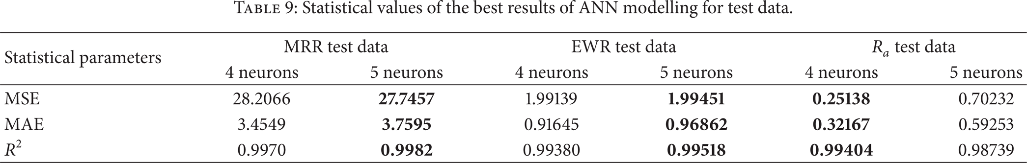
Statistical parameters of ANN models are presented in Tables 8 and 9, where; R², MSE, and MAE correspond to the coefficient of correlation, mean square error and the mean absolute error. Table 8 shows the performances of the best ANN models for training phase. Table 9 shows the performances of the best ANN models for test data which consists of test and validation data. The patterns used in test and training sets are selected in systematic randomly. It seems that the network with 5 neurons in its hidden layer has better performance than the network with 4 neurons in its hidden layer for all training phases. On the other hand, though, the former has better performance for MMR and EWR test data, and the latter has showed better performance for R_a test data.

Table 8:

Statistical values of the best results of ANN modelling for training data.

Statistical parameters	MRR train data		EWR train data		R_a train data
Statistical parameters	4 neurons	5 neurons	4 neurons	5 neurons	4 neurons	5 neurons

MSE	11.0836	3.4706	0.58164	0.01511	0.01345	0.00134
MAE	2.2148	1.3690	0.52516	0.10309	0.08537	0.02819
R ²	0.9994	0.9998	0.99718	0.99993	0.99911	0.99991

Table 9:

Statistical values of the best results of ANN modelling for test data.

Statistical parameters	MRR test data		EWR test data		R_a test data
Statistical parameters	4 neurons	5 neurons	4 neurons	5 neurons	4 neurons	5 neurons

MSE	28.2066	27.7457	1.99139	1.99451	0.25138	0.70232
MAE	3.4549	3.7595	0.91645	0.96862	0.32167	0.59253
R ²	0.9970	0.9982	0.99380	0.99518	0.99404	0.98739

3.3. Development of Adaptive Nero-Fuzzy Inference System (ANFIS) Models

Fuzzy logic (FL) and neural networks (NN) supply two different methodologies to achieve an appropriate solution for uncertainty. Appropriate hybridization of fuzzy logic and neural networks technologies lead to overcoming the weakness of one with the strength of the other and so provide efficient solution to a range of problems belonging to different domains. A specific approach in Neuro-Fuzzy development is the Adaptive Neuro-Fuzzy Inference System (ANFIS) [29 –31]. The ANFIS learning method works similarly to the neural networks' one. In ANFIS system, membership functions parameters are adjusted using either a backpropagation algorithm alone or in combination with a least squares type of method by using a given input/output data set. This adjustment allows your fuzzy systems to learn from the data from modelling [29].

Figure 5 shows a typical ANFIS architecture with two inputs (x and y), the linguistic labels (A1, A2, B1, and B2) associated with this node function, the normalized firing strengths (W_i), and the node label (Π). ANFIS is a Sugeno-type fuzzy system in five-layered feed-forward network structure. A fuzzification process is performed in the first layer, the second layer is the rule layer, and each neuron in this layer corresponds to a single Sugeno-type fuzzy rule. The membership functions (MFs) are normalized in the third layer. The fourth layer is defuzzification layer where the consequent parts of the rules are executed. The fifth layer computes the overall ANFIS output as the summation of all input signals [32].

Figure 5:

A typical ANFIS architecture [29].

In this study, to build an ANFIS model and to predict the MRR, EWR, and R_a, the Adaptive Nero-Fuzzy Inference System (ANFIS) editor of MATLAB was used. The toolbox helps you to create fuzzy systems by using a backpropagation algorithm alone or in combination with a least squares method. Training and testing data set used in ANFIS models are the same as those used in ANN and GEP models. Here, testing data set was used as a checking data set. A checking data set is employed for verifying the ANFIS model generalization capabilities, except for training set. An initial FIS for training of ANFIS implementing subtractive clustering on the input/output data given is created by the model. A fast identification of parameters is obtained by using the hybrid learning algorithm so the necessary time to approach the convergence is reduced.

A membership function (MF) is a curve that defines how each point in the input space is mapped to a membership value (or degree of membership) between 0 and 1. The ANFIS toolbox includes 11 built-in membership function types: trimf, trapmf, gauss, bell, and so forth. The number of membership functions, MFs, and the type of input and output membership functions are chosen in the toolbox. In this study, due to their smoothness and concise notation, Gaussian and bell membership functions were chosen for inputs. The numbers of MFs were changed from 3-3-3 to 6-6-6. It means that 64 × 2 = 128 tries were carried out for each performance parameter. MF type was selected linear as the output membership function and epoch number was taken as 100.

Tables 10 and 11 show statistically the performances of the best ANFIS models that have Gaussian and bell membership functions for training and test phase, respectively. After training and testing, the number of MFs was fixed for each input variable, when the ANFIS model reaches the more acceptable satisfactory level at gauss MFs. For the best models, ANFIS architectures are illustrated in Table 12.

Table 10:

Statistical values of the best results of ANFIS modelling for training data.

Statistical parameters	MRR train data		EWR train data		R_a train data
Statistical parameters	GbellMF's (434)	GaussMF's (434)	GbellMF's (666)	GaussMF's (666)	GbellMF's (343)	GaussMF's (444)

MSE	37.4509	1.9850	0.0162	1.9852	0.0330	0.0100
MAE	3.0676	0.7010	2.8726	0.7009	0.1081	0.0420
R ²	0.9979	0.9999	0.9999	0.9999	0.9978	0.9996

Table 11:

Statistical values of the best results of ANFIS modelling for testing data.

Statistical parameters	MRR test data		EWR test data		R_a test data
Statistical parameters	GbellMF's (434)	GaussMF's (434)	GbellMF's (666)	GaussMF's (666)	GbellMF's (343)	GaussMF's (444)

MSE	72.0726	71.5620	0.0013	1.4000	1.9228	0.0670
MAE	5.5172	5.5080	14.4491	0.9860	0.6852	0.1780
R ²	0.9944	0.9944	0.9632	0.9961	0.9738	0.9973

Table 12:

ANFIS architecture and training parameters.

MFs type	MRR	EWR	R _a
MFs type	Gauss	Gauss	Gauss

Number of nodes	124	474	158
Number of linear parameters	192	864	256
Number of nonlinear parameters	22	36	36
Total number of parameters	214	900	292
Number of fuzzy rules	48	216	64
NumMFs input 1	4	6	4
NumMFs input 2	3	6	4
NumMFs input 3	4	6	4

Table 13:

Statistical values of MRR modelling for training and testing sets.

Statistical parameters	MRR training sets			MRR test sets
Statistical parameters	GEP	ANN	ANFIS	GEP	ANN	ANFIS

MSE	55.352	3.4706	1.985	162.236	27.7457	71.562
MAE	5.486	1.3690	0.701	8.352	3.7595	5.508
R ²	0.9968	0.9998	0.9999	0.9958	0.9982	0.9944

Table 14:

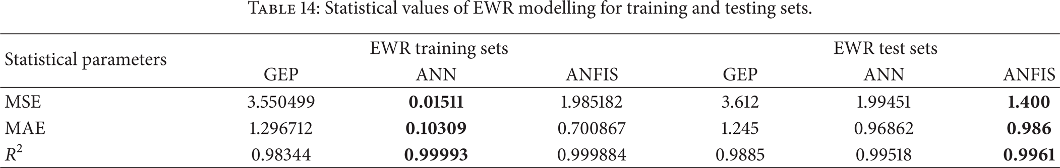
Statistical values of EWR modelling for training and testing sets.

Statistical parameters	EWR training sets			EWR test sets
Statistical parameters	GEP	ANN	ANFIS	GEP	ANN	ANFIS

MSE	3.550499	0.01511	1.985182	3.612	1.99451	1.400
MAE	1.296712	0.10309	0.700867	1.245	0.96862	0.986
R ²	0.98344	0.99993	0.999884	0.9885	0.99518	0.9961

Table 15:

Statistical values of R_a modelling for training and testing sets.

Statistical Parameters	R_a Training Sets			R_a Test sets
Statistical Parameters	GEP	ANN	ANFIS	GEP	ANN	ANFIS

MSE	0.1000	0.0100	0.0100	0.2200	0.25138	0.0670
MAE	0.2360	0.0850	0.0420	0.3380	0.32167	0.1780
R ²	0.9936	0.9991	0.9996	0.9942	0.99404	0.9973

Table 16:

Training evaluation values of electrode wear rate (EWR).

Number	I	T _on	T _off	Experiment	GEP		ANN		ANFIS
Number	(A)	(μs)	(μs)	Experiment	Guess	Ratio	Guess	Ratio	Guess	Ratio

1	3	3	3	15.00	18.68	0.80	15.0	1.00	15.0	1.00
2	3	12	3	4.00	5.25	0.76	3.9	1.02	4.0	1.00
3	3	25	6	1.30	1.76	0.74	1.2	1.06	1.3	1.00
4	3	100	24	0.50	0.15	3.32	0.4	1.32	0.5	1.00
5	6	6	3	28.00	22.40	1.25	27.8	1.01	27.9	1.00
6	6	12	3	15.00	13.51	1.11	15.1	0.99	15.1	0.99
7	6	24	6	6.00	6.53	0.92	6.1	0.98	5.9	1.02
8	6	48	6	2.00	2.61	0.77	2.1	0.97	2.0	1.00
9	6	99	12	0.80	0.84	0.95	0.6	1.38	0.8	1.00
10	12.5	3	3	38.00	37.67	1.01	38.2	1.00	38.0	1.00
11	12.5	12	3	24.00	23.88	1.00	23.9	1.01	24.0	1.00
12	12.5	24	6	13.00	15.02	0.87	12.9	1.00	13.0	1.00
13	12.5	48	6	4.80	8.04	0.60	4.8	0.99	4.9	0.98
14	12.5	201	24	0.10	1.30	0.08	0.3	0.33	0.1	1.00
15	12.5	402	48	0.10	0.43	0.23	0.1	1.16	0.1	1.00
16	25	3	3	40.00	42.06	0.95	39.9	1.00	40.0	1.00
17	25	6	3	38.00	38.57	0.99	38.2	1.00	38.1	1.00
18	25	24	6	24.00	24.00	1.00	24.0	1.00	23.9	1.00
19	25	48	6	14.00	15.59	0.90	13.9	1.01	14.1	0.99
20	25	99	12	6.00	8.54	0.70	6.2	0.96	6.0	1.00
21	25	201	24	2.20	4.11	0.54	2.1	1.06	2.2	1.00
22	25	801	99	0.10	0.65	0.15	0.1	1.30	0.1	1.00
23	50	3	3	45.00	44.52	1.01	44.8	1.00	45.0	1.00
24	50	12	3	38.00	38.50	0.99	38.2	1.00	38.0	1.00
25	50	24	6	32.00	32.12	1.00	32.0	1.00	32.0	1.00
26	50	48	6	25.00	24.08	1.04	24.9	1.00	25.0	1.00
27	50	99	12	20.00	15.53	1.29	20.1	1.00	20.0	1.00
28	50	201	24	10.00	8.88	1.13	9.9	1.01	10.0	1.00
29	50	402	48	4.50	4.59	0.98	4.6	0.98	4.5	1.00
30	50	801	99	1.40	2.14	0.65	1.4	1.00	1.4	1.00

Table 17:

Test values of electrode wear ratio (EWR).

Number	I	T _on	T _off	Experiment	GEP		ANN		ANFIS
Number	(A)	(μs)	(μs)	Experiment	Guess	Ratio	Guess	Ratio	Guess	Ratio

1	3	6	3	12.00	11.54	1.04	9.67	1.24	11.84	1.01
2	3	50	12	0.50	0.54	0.93	0.37	1.35	0.87	0.58
3	6	3	3	35.00	29.75	1.18	32.94	1.06	33.03	1.06
4	6	201	24	0.10	0.24	0.41	0.25	0.39	0.10	0.98
5	12.5	6	3	33.00	32.21	1.02	33.43	0.99	34.16	0.97
6	12.5	99	12	1.70	3.49	0.49	1.47	1.16	2.25	0.75
7	25	12	3	31.00	32.32	0.96	32.22	0.96	32.63	0.95
8	25	402	48	0.40	1.75	0.23	0.21	1.91	1.53	0.26
9	50	6	3	42.00	42.51	0.99	41.58	1.01	43.11	0.97
10	50	801	99	0.01	0.89	0.11	0.18	0.54	1.88	0.05

4. Results and Discussion

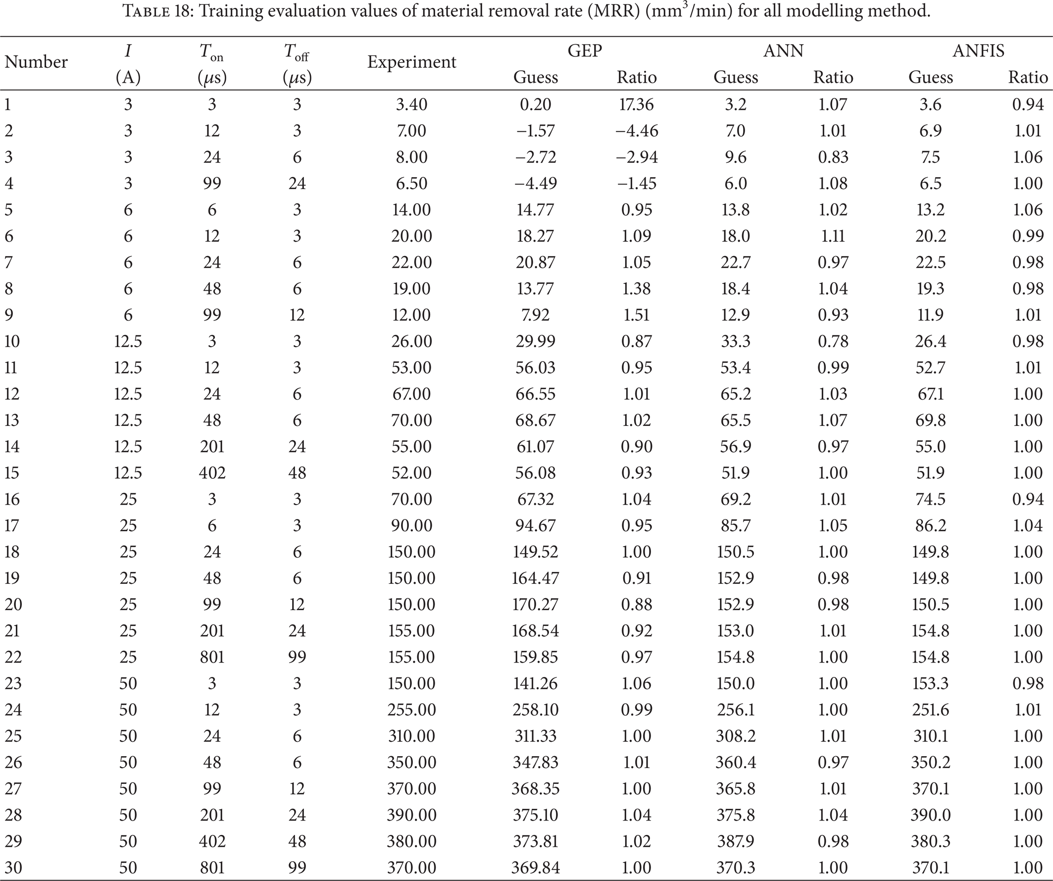
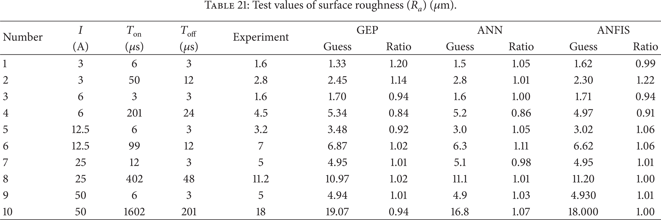
The results obtained from the modelling and experimental studies are compared in this section. Experimental data are illustrated experiment, and data obtained from modelling studies are illustrated as guess value at Tables 16 –21. Training data sets for MRR, EWR, and R_a responses are given at Tables 16, 18, and 20 and testing data are given at Tables 17, 19, and 21, respectively. Ratio means rate of the experimental data to the predicted value obtained from modelling study. Estimation capabilities of all artificial models for each experimental data can be evaluated as quantitatively with the help of ratio values.

Table 18:

Training evaluation values of material removal rate (MRR) (mm³/min) for all modelling method.

Number	I	T _on	T _off	Experiment	GEP		ANN		ANFIS
Number	(A)	(μs)	(μs)	Experiment	Guess	Ratio	Guess	Ratio	Guess	Ratio

1	3	3	3	3.40	0.20	17.36	3.2	1.07	3.6	0.94
2	3	12	3	7.00	−1.57	−4.46	7.0	1.01	6.9	1.01
3	3	24	6	8.00	−2.72	−2.94	9.6	0.83	7.5	1.06
4	3	99	24	6.50	−4.49	−1.45	6.0	1.08	6.5	1.00
5	6	6	3	14.00	14.77	0.95	13.8	1.02	13.2	1.06
6	6	12	3	20.00	18.27	1.09	18.0	1.11	20.2	0.99
7	6	24	6	22.00	20.87	1.05	22.7	0.97	22.5	0.98
8	6	48	6	19.00	13.77	1.38	18.4	1.04	19.3	0.98
9	6	99	12	12.00	7.92	1.51	12.9	0.93	11.9	1.01
10	12.5	3	3	26.00	29.99	0.87	33.3	0.78	26.4	0.98
11	12.5	12	3	53.00	56.03	0.95	53.4	0.99	52.7	1.01
12	12.5	24	6	67.00	66.55	1.01	65.2	1.03	67.1	1.00
13	12.5	48	6	70.00	68.67	1.02	65.5	1.07	69.8	1.00
14	12.5	201	24	55.00	61.07	0.90	56.9	0.97	55.0	1.00
15	12.5	402	48	52.00	56.08	0.93	51.9	1.00	51.9	1.00
16	25	3	3	70.00	67.32	1.04	69.2	1.01	74.5	0.94
17	25	6	3	90.00	94.67	0.95	85.7	1.05	86.2	1.04
18	25	24	6	150.00	149.52	1.00	150.5	1.00	149.8	1.00
19	25	48	6	150.00	164.47	0.91	152.9	0.98	149.8	1.00
20	25	99	12	150.00	170.27	0.88	152.9	0.98	150.5	1.00
21	25	201	24	155.00	168.54	0.92	153.0	1.01	154.8	1.00
22	25	801	99	155.00	159.85	0.97	154.8	1.00	154.8	1.00
23	50	3	3	150.00	141.26	1.06	150.0	1.00	153.3	0.98
24	50	12	3	255.00	258.10	0.99	256.1	1.00	251.6	1.01
25	50	24	6	310.00	311.33	1.00	308.2	1.01	310.1	1.00
26	50	48	6	350.00	347.83	1.01	360.4	0.97	350.2	1.00
27	50	99	12	370.00	368.35	1.00	365.8	1.01	370.1	1.00
28	50	201	24	390.00	375.10	1.04	375.8	1.04	390.0	1.00
29	50	402	48	380.00	373.81	1.02	387.9	0.98	380.3	1.00
30	50	801	99	370.00	369.84	1.00	370.3	1.00	370.1	1.00

Table 19:

Test values of material removal rate (MRR) (mm³/min).

Number	I	T _on	T _off	Experiment	GEP		ANN		ANFIS
Number	(A)	(μs)	(μs)	Experiment	Guess	Ratio	Guess	Ratio	Guess	Ratio

1	3	6	3	5.00	0.61	8.21	4.98	1.00	5.07	0.99
2	3	48	12	8.00	−3.71	−2.08	8.31	0.93	13.53	0.57
3	6	3	3	10.00	10.01	1.00	10.55	0.95	10.88	0.92
4	6	201	24	7.00	2.46	2.85	5.59	1.25	3.36	2.08
5	12.5	6	3	36.00	42.84	0.84	41.17	0.87	36.97	0.97
6	12.5	99	12	62.00	66.36	0.93	61.98	1.00	58.50	1.06
7	25	12	3	130.00	124.34	1.05	114.71	1.13	122.46	1.06
8	25	402	48	155.00	163.70	0.95	154.08	1.01	177.06	0.88
9	50	6	3	195.00	196.89	0.99	183.70	1.06	205.53	0.95
10	50	801	99	330.00	365.71	0.90	330.23	1.00	329.94	1.00

Table 20:

Training values of surface roughness (R_a) (μm).

Number	I	T _on	T _off	Experiment	GEP		ANN		ANFIS
Number	(A)	(μs)	(μs)	Experiment	Guess	Ratio	Guess	Ratio	Guess	Ratio

1	3	3	3	1.40	0.89	1.57	1.40	1.00	1.39	1.01
2	3	12	3	2.00	1.80	1.11	1.96	1.02	2.00	1.00
3	3	24	6	2.20	1.84	1.20	2.22	0.99	2.21	1.00
4	3	99	24	3.20	3.24	0.99	3.20	1.00	3.20	1.00
5	6	6	3	2.00	2.18	0.92	2.00	1.00	2.02	0.99
6	6	12	3	2.50	2.74	0.91	2.45	1.02	2.50	1.00
7	6	24	6	2.80	3.04	0.92	2.84	0.99	2.79	1.00
8	6	48	6	3.50	3.82	0.92	3.44	1.02	3.49	1.00
9	6	99	12	4.00	4.20	0.95	4.05	0.99	4.00	1.00
10	12.5	3	3	2.20	2.19	1.01	2.20	1.00	2.32	0.95
11	12.5	12	3	4.00	4.16	0.96	4.00	1.00	4.09	0.98
12	12.5	24	6	5.00	4.95	1.01	4.97	1.01	4.99	1.00
13	12.5	48	6	5.60	5.89	0.95	5.65	0.99	5.94	0.94
14	12.5	201	24	8.00	7.48	1.07	7.98	1.00	7.99	1.00
15	12.5	402	48	9.00	9.07	0.99	9.00	1.00	9.00	1.00
16	25	3	3	3.20	3.30	0.97	3.28	0.97	3.28	0.98
17	25	6	3	4.00	4.15	0.96	3.94	1.01	3.92	1.02
18	25	24	6	5.60	5.89	0.95	5.62	1.00	5.63	0.99
19	25	48	6	7.00	7.00	1.00	6.99	1.00	7.00	1.00
20	25	99	12	8.00	8.39	0.95	7.97	1.00	7.99	1.00
21	25	201	24	10.00	9.95	1.00	10.02	1.00	9.85	1.02
22	25	801	99	12.60	13.21	0.95	12.60	1.00	12.60	1.00
23	50	3	3	4.00	4.01	1.00	3.96	1.01	4.05	0.99
24	50	12	3	6.30	5.89	1.07	6.35	0.99	6.32	1.00
25	50	24	6	7.00	7.00	1.00	6.98	1.00	7.02	1.00
26	50	48	6	9.00	8.32	1.08	8.95	1.01	8.98	1.00
27	50	99	12	10.00	9.97	1.00	10.07	0.99	10.12	0.99
28	50	201	24	12.60	11.91	1.06	12.56	1.00	12.60	1.00
29	50	402	48	14.00	14.16	0.99	14.00	1.00	14.05	1.00
30	50	801	99	16.00	15.88	1.01	16.00	1.00	16.00	1.00

Table 21:

Test values of surface roughness (R_a) (μm).

Number	I	T _on	T _off	Experiment	GEP		ANN		ANFIS
Number	(A)	(μs)	(μs)	Experiment	Guess	Ratio	Guess	Ratio	Guess	Ratio

1	3	6	3	1.6	1.33	1.20	1.5	1.05	1.62	0.99
2	3	50	12	2.8	2.45	1.14	2.8	1.01	2.30	1.22
3	6	3	3	1.6	1.70	0.94	1.6	1.00	1.71	0.94
4	6	201	24	4.5	5.34	0.84	5.2	0.86	4.97	0.91
5	12.5	6	3	3.2	3.48	0.92	3.0	1.05	3.02	1.06
6	12.5	99	12	7	6.87	1.02	6.3	1.11	6.62	1.06
7	25	12	3	5	4.95	1.01	5.1	0.98	4.95	1.01
8	25	402	48	11.2	10.97	1.02	11.1	1.01	11.20	1.00
9	50	6	3	5	4.94	1.01	4.9	1.03	4.930	1.01
10	50	1602	201	18	19.07	0.94	16.8	1.07	18.000	1.00

Comparisons of the training performances and testing performances of all models with the experimental equivalents are given as graphically in Figures 6 and 7. As shown in these figures, there is a little deviation between the real and predicted values. It means that all of these models can predict accurately and satisfactorily EDM performances by learning complex relationship between the input and output parameters.

Figure 6:

Comparisons of training performance of all methods for (a) MRR, (b) EWR, and (c) R_a prediction.

Figure 7:

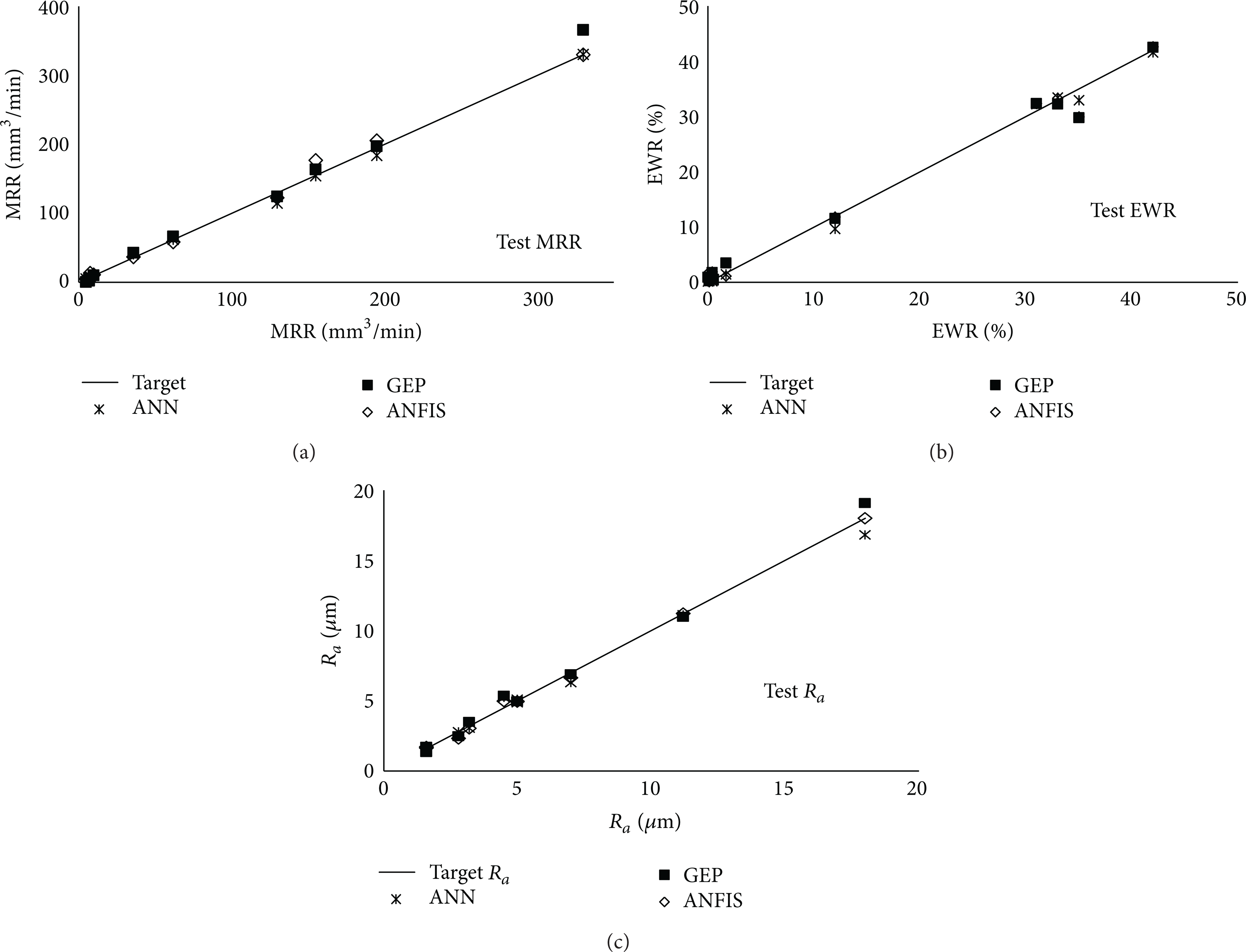
Comparisons of testing performance of all methods for (a) MRR, (b) EWR, and (c) R_a prediction.

MSE, MAE, and R² values are used to compare statistically the created models. Statistical performances of MRR, EWR, and R_a modelling for training and testing sets are given at Tables 13, 14, and 15, respectively. Although the ANFIS model is very successful in training (R² = 0.9999, MAE = 0.701, and MSE = 1.985), the ANN model is better in prediction of MRR (R² = 0.9982, MAE = 3.7595, and MSE = 27.7457) (Table 13). For EWR modelling, the ANN model is more successful in training than the ANFIS model but the ANFIS model is slightly better in prediction of EWR than the ANN model (Table 14). The ANFIS model is the best for training and prediction of R_a in all models (Table 15).

GEP model is less successful compared with other models. In prediction of EWR and R_a, the ANFIS model is the best as shown in Tables 13 and 14. All models are better in prediction of R_a than MRR. The differences between the ANN and the ANFIS results in terms of R², MSE, and MAE, are very close, so that both models may be accepted as successful. However, the ANFIS model is slightly better than the ANN and the GEP model.

5. Conclusion

In this paper, a comprehensive study to compare the performances of GEP, ANN, and ANFIS approaches on modelling of important EDM performances was realized. Three basic parameters discharge current (I), pulse on-time (T_on), and pulse off-time (T_off) were input parameters while material removing rate (MRR), electrode wear ratio (EWR), and surface roughness (R_a) were the output parameters. A series of experiments was carried out using DIN 1.2080 tool steel and copper electrode. The data set obtained from experimental study was used to develop mathematical models.

The results show that all approaches are successful for prediction of EDM performances by learning complex relationship between the input and output parameters in terms of statistical parameters.

GEP model was less successful among others; however, it has a simple and explicit mathematical formulation.

The results produced by both ANN and ANFIS models also present relatively good level of accuracy. However, the ANFIS model is slightly more successful than the ANN model.

Modeling of R_a is more efficient compared to other EDM performances.

Using of MLP with back-propagation learning algorithm (while it has one hidden layer, TanhAxon, and 5 neurons) is successful for modelling EDM performances.

Selection of gauss MFs type gives better results than the others MFs types for modelling of EDM performances by using ANFIS method.

Footnotes

Acknowledgment

The authors would like to thank the Scientific Research Projects (BAP) Unit of Gaziantep University for supporting this study.

References

Wang

Chow

Yang

, and Lu

, “Recast layer removal after electrical discharge machining via Taguchi analysis: a feasibility study,” Journal of Materials Processing Technology, vol. 209, no. 8, pp. 4134–4140, 2009.

Mandal

Pal

S. K.

, and Saha

, “Modeling of electrical discharge machining process using back propagation neural network and multi-objective optimization using non-dominating sorting genetic algorithm—II,” Journal of Materials Processing Technology, vol. 186, no. 1–3, pp. 154–162, 2007.

Lee

S. H.

and Li

X. P.

, “Study of the effect of machining parameters on the machining characteristics in electrical discharge machining of tungsten carbide,” Journal of Materials Processing Technology, vol. 115, no. 3, pp. 344–358, 2001.

Jain

N. K.

and Jain

V. K.

, “Modeling of material removal in mechanical type advanced machining processes: a state-of-art review,” International Journal of Machine Tools and Manufacture, vol. 41, no. 11, pp. 1573–1635, 2001.

Mohd Abbas

Solomon

D. G.

, and Fuad Bahari

, “A review on current research trends in electrical discharge machining (EDM),” International Journal of Machine Tools and Manufacture, vol. 47, no. 7–8, pp. 1214–1228, 2007.

Indurkhya

and Rajurkar

K. P.

, “Artificial Neural Network approach in modelling of EDM process,” in Proceedings of the Artificial Neural 'Networks in Engineering (ANNIE '92), pp. 845–850, November 1992.

Tsai

and Wang

, “Comparisons of neural network models on material removal rate in electrical discharge machining,” Journal of Materials Processing Technology, vol. 117, no. 1–2, pp. 111–124, 2001.

Tsai

K. M.

and Wang

P. J.

, “Predictions on surface finish in electrical discharge machining based upon neural network models,” International Journal of Machine Tools and Manufacture, vol. 41, no. 10, pp. 1385–1403, 2001.

Lin

C. L.

Lin

J. L.

, and Ko

T. C.

, “Optimisation of the EDM process based on the orthogonal array with fuzzy logic and grey relational analysis method,” International Journal of Advanced Manufacturing Technology, vol. 19, no. 4, pp. 271–277, 2002.

10.

Wang

Gelgele

H. L.

Wang

Yuan

, and Fang

, “A hybrid intelligent method for modelling the EDM process,” International Journal of Machine Tools and Manufacture, vol. 43, no. 10, pp. 995–999, 2003.

11.

Panda

D. K.

and Bhoi

R. K.

, “Artificial neural network prediction of material removal rate in electro discharge machining,” Materials and Manufacturing Processes, vol. 20, no. 4, pp. 645–672, 2005.

12.

Yilmaz

Eyercioglu

, and Gindy

N. N. Z.

, “A user-friendly fuzzy-based system for the selection of electro discharge machining process parameters,” Journal of Materials Processing Technology, vol. 172, no. 3, pp. 363–371, 2006.

13.

Salman

Ö.

and Kayacan

M. C.

, “Evolutionary programming method for modeling the EDM parameters for roughness,” Journal of Materials Processing Technology, vol. 200, no. 1–3, pp. 347–355, 2008.

14.

Rao

G. K. M.

Janardhana

G. R

Rao

D H.

, and Rao

M. S.

, “Development of hybrid model and optimization of surface roughness in electric discharge machining using artificial neural networks and genetic algorithm,” Journal of Materials Processing Technology, vol. 209, no. 3, pp. 1512–1520, 2009.

15.

Maji

and Pratihar

D. K.

, “Forward and reverse mappings of electrical discharge machining process using adaptive network-based fuzzy inference system,” Expert Systems with Applications, vol. 37, no. 12, pp. 8566–8574, 2010.

16.

Joshi

S. N.

and Pande

S. S.

, “Intelligent process modeling and optimization of die-sinking electric discharge machining,” Applied Soft Computing Journal, vol. 11, no. 2, pp. 2743–2755, 2011.

17.

K. H.

and Newman

S. T.

, “State of the art electrical discharge machining (EDM),” International Journal of Machine Tools and Manufacture, vol. 43, no. 13, pp. 1287–1300, 2003.

18.

Kunieda

Lauwers

Rajurkar

K. P.

, and Schumacher

B. M.

, “Advancing EDM through fundamental insight into the process,” CIRP Annals, vol. 54, no. 2, pp. 599–622, 2005.

19.

Guu

Y. H.

Chou

C. Y.

, and Chiou

, “Study of the effect of machining parameters on the machining characteristics in electrical discharge machining of Fe-Mn-Al alloy,” Materials and Manufacturing Processes, vol. 20, no. 6, pp. 905–916, 2005.

20.

Ong

C. S.

Huang

J. J.

, and Tzeng

G. H.

, “Building credit scoring models using genetic programming,” Expert Systems with Applications, vol. 29, no. 1, pp. 41–47, 2005.

21.

Cevik

and Guzelbey

I. H.

, “A soft computing based approach for the prediction of ultimate strength of metal plates in compression,” Engineering Structures, vol. 29, no. 3, pp. 383–394, 2007.

22.

Kök

Kanca

, and Eyercioglu

Ö.

, “Prediction of surface roughness in abrasive waterjet machining of particle reinforced MMCs using genetic expression programming,” International Journal of Advanced Manufacturing Technology, vol. 55, no. 9–12, pp. 955–968, 2011.

23.

Koza

J. R.

, “Genetic programming as a means for programming computers by natural selection,” Statistics and Computing, vol. 4, no. 2, pp. 87–112, 1994.

24.

Ferreira

, “Gene expression programming: a new adaptive algorithm for solving problems,” Complex Systems, vol. 13, no. 2, pp. 87–129, 2001.

25.

Cevik

, “Genetic programming based formulation of rotation capacity of wide flange beams,” Journal of Constructional Steel Research, vol. 63, no. 7, pp. 884–893, 2007.

26.

Haykin

, Neural Networks and Learning Machines, Prentice Hall, Upper Saddle River, NJ, USA, 3rd edition, 2009.

27.

Rafiq

M. Y.

Bugmann

, and Easterbrook

D. J.

, “Neural network design for engineering applications,” Computers and Structures, vol. 79, no. 17, pp. 1541–1552, 2001.

28.

Guzelbey

I. H.

Cevik

, and Erklig

, “Prediction of web crippling strength of cold-formed steel sheetings using neural networks,” Journal of Constructional Steel Research, vol. 62, no. 10, pp. 962–973, 2006.

29.

Jang

J. S. R.

, “ANFIS: adaptive-network-based fuzzy inference system,” IEEE Transactions on Systems, Man and Cybernetics, vol. 23, no. 3, pp. 665–685, 1993.

30.

Jang

J. S. R.

Sun

T. G.

, and Mizutani

, Neuro-Fuzzy and Soft Computing: A computational Approach to Learning and Machine Intelligence, Prentice Hall, 1997.

31.

Kim

and Kasabov

, “HyFIS: adaptive neuro-fuzzy inference systems and their application to nonlinear dynamical systems,” Neural Networks, vol. 12, no. 9, pp. 1301–1319, 1999.

32.

Sugeno

and Kang

G. T.

, “Structure identification of fuzzy model,” Fuzzy Sets and Systems, vol. 28, no. 1, pp. 15–33, 1988.

Comparison of Soft Computing Techniques for Modelling of the EDM Performance Parameters

Abstract

1. Introduction

2. Experimental Studies

3. Modelling Study

3.1. Development of Genetic Programming (GP) Models

3.2. Development of Artificial Neural Networks (ANN) Models

3.3. Development of Adaptive Nero-Fuzzy Inference System (ANFIS) Models

4. Results and Discussion

5. Conclusion

Footnotes

Acknowledgment

References