Sage Journals: Discover world-class research

Abstract

The stochastic dynamic problems were becoming more difficult after considering the influences of stochastic factors and the complexity of the dynamic problems. To this background, the finite volume method combined with Perturbation Method was proposed for the stochastic dynamic analysis. The equations of perturbation-finite volume method were derived; the explicit expressions between random response and basic random variables were given; the method of stochastic dynamic analysis was discussed; and the examples were presented to verify the perturbation-finite volume method. The results of perturbation-finite volume method were compared with the results of Monte Carlo Method, which proved that the proposed method was correct and accurate. Because the proposed method was simple and clear, the equations were easy to establish and the efficiency was improved. Meanwhile, the proposed method was successfully applied to the stochastic dynamic analysis of linear multibody system, which was verified through the example in this paper.

1. Introduction

In recent years, it has been gradually accepted by workers and engineers that various random factors should be considered in structural analysis and design. In this context, stochastic structural analysis has become a hot topic in the field [1 –12]. The problems of static stochastic structural analysis can be solved very well, and it has been applied to engineering practice successfully. However, the study of the stochastic dynamic analysis was still in the primary stage [13 –19]. The main reasons were that the issues of stochastic dynamic analysis were difficult; there were many problems and even some of the basic problems are still to be studied. For example, the stochastic dynamic response is difficult to solve; the explicit expressions between random response and basic random variables are difficult to give and so on.

Currently, the effective solution methods for stochastic dynamic problems were mostly stochastic simulations based on dynamics analysis. The finite element method was applied mostly in the dynamic problems, and the calculation time was longer. The stochastic dynamic analysis in the time and space domain was random; the stochastic simulation based on the finite element method will lead to the low-solving efficiency. When using semianalytical methods to solve the problem of stochastic dynamic analysis, the main difficulty was that the methods of dynamic analysis such as the finite element method were mostly based on implicit solution. It was difficult to give the explicit expressions between random response and basic random variables, and it was difficult to obtain the sensitivity information. Therefore, it was difficult to carry out the stochastic dynamic analysis.

To solve these problems, Finite volume method combined with perturbation method was proposed for the stochastic dynamic analysis, and the method was successfully applied to the stochastic dynamic analysis of linear multibody system. The finite volume method was originally used in computational fluid mechanics; the application in the field of solid mechanics has only been considered in recent years, and it has been successfully applied in many engineering practical problems [20, 21]. However, the finite volume method is mostly studied on the problems of solid mechanics for deterministic variables. For stochastic problems, it has been rarely reported in the field of solid mechanics. The advantage of finite volume method was that the explicit expressions between random response and basic random variables could be given, which was essential for the stochastic dynamic analysis. Therefore, finite volume method combined with perturbation method was proposed for the stochastic dynamic analysis.

2. The Equations of Finite Volume Method

The process of solution for finite volume method was that the solution domain was partitioned into finite continuous grids, to form a nonoverlapping control volume which surrounds each grid point according to certain rules; the governing equations were integrated in the control volume to form the discrete equations. Explicit central difference scheme was used in time field. First, the acceleration of every control volume was calculated by governing equations. The velocity and displacement of every control volume were calculated by central difference method, and then the grid stress was calculated. Finally, the stress was taken back to the governing equations for the next time step.

The governing equations of finite volume method were the mass, momentum, and energy conservation equations. Discretization was mainly focused on the momentum conservation equations; the governing equations were integrated in the control volume. For three-dimensional solid structure, three-dimensional unstructured grid was used as shown in Figure 1; connecting the gravity of the tetrahedron, the center of each side, and the midpoint of each edge, which comprised six planes. The tetrahedron was divided into four parts by the six planes, and each part was the part of the control volume.

Figure 1:

Three-dimensional unstructured grid.

The governing equations were integrated in the control volume:

\int_{V} ρ {\overset{‥}{u}}_{i} d V = \int_{V} (ρ b_{i} + \frac{\partial σ_{j i}}{\partial x_{j}}) d V .

(1)

Here, u_i (i = 1, 2, 3) was the displacement component of the control volume and ρ was the material density. When all of the control volumes satisfied (1), the solution domain naturally satisfied the momentum conservation. If the body force was ignored, the volume integral was converted into surface integral through the Gauss formula. Equation (1) could be written as:

ρ {\overset{‥}{u}}_{i} \int_{V} d V = \oint_{S} σ_{j i} n_{j} d S,

(2)

where n_j (j = 1, 2, 3) was the unit vector component on the outward normal direction for the control volume. For node 1 in Figure 1, if it was connected with m tetrahedral, the left integral of (2) could be expressed as

ρ {\overset{‥}{u}}_{i} \int_{V} d V = \frac{{\overset{‥}{u}}_{i}}{4} \sum_{n = 1}^{m} M_{n},

(3)

where M_n was the quality of the n tetrahedral.

Supposing that the stress of tetrahedral was constant, then the stress on the boundary of the control volume was constant. Because the surface of the control volume was formed by some planes, the unit vector components on the outward normal direction for the control volume were constant. For the node 1 in Figure 1, it is connected with m tetrahedral and accumulated the integrals of m tetrahedral; the final form could be expressed as

\frac{{\overset{‥}{u}}_{i}}{4} \sum_{n = 1}^{m} M_{n} = \sum_{n = 1}^{m} {(a_{1} σ_{1 i})}_{n} + \sum_{n = 1}^{m} {(a_{2} σ_{2 i})}_{n} + \sum_{n = 1}^{m} {(a_{3} σ_{3 i})}_{n} .

(4)

Here, a₁, a₂, and a₃ were the coefficients of the n tetrahedral which was connected with node 1. Its value was related to the node coordinates of the tetrahedral. For other nodes, it had the same expressions. We have

\begin{matrix} a_{1} = - \frac{1}{6} | \begin{vmatrix} 1 & 1 & 1 \\ y_{4} & y_{3} & y_{2} \\ z_{4} & z_{3} & z_{2} \end{vmatrix} |, \\ a_{2} = - \frac{1}{6} | \begin{vmatrix} 1 & 1 & 1 \\ z_{4} & z_{3} & z_{2} \\ x_{4} & x_{3} & x_{2} \end{vmatrix} |, \\ a_{3} = - \frac{1}{6} | \begin{vmatrix} 1 & 1 & 1 \\ x_{4} & x_{3} & x_{2} \\ y_{4} & y_{3} & y_{2} \end{vmatrix} | . \end{matrix}

(5)

Equation (4) in matrix form is as follows:

\overset{‥}{u} = \frac{1}{M} \sum_{n = 1}^{m} A_{n} σ_{n},

(6)

where ρ was the material density M was the quality of the control volume. We have

\begin{matrix} \overset{‥}{u} = {[\begin{bmatrix} {\overset{‥}{u}}_{1} & {\overset{‥}{u}}_{2} & {\overset{‥}{u}}_{3} \end{bmatrix}]}^{T}, \\ σ_{n} = {[\begin{bmatrix} σ_{11} & σ_{22} & σ_{33} & σ_{12} & σ_{23} & σ_{31} \end{bmatrix}]}^{T}, \\ A_{n} = \frac{1}{6} [\begin{bmatrix} a_{1} & 0 & 0 & a_{2} & 0 & a_{3} \\ 0 & a_{2} & 0 & a_{1} & a_{3} & 0 \\ 0 & 0 & a_{3} & 0 & a_{2} & a_{1} \end{bmatrix}] . \end{matrix}

(7)

The boundary conditions and the initial conditions were given as follows.

Boundary conditions are as follows:

σ \cdot n = \bar{X}, u = \bar{u},

(8)

where $\bar{X}$ was the outside force of boundary and $\bar{u}$ was the displacement of boundary.

Initial conditions are as follows:

u |_{t = 0} = u_{0}, \dot{u} |_{t = 0} = {\dot{u}}_{0} .

(9)

Explicit central difference scheme was used in time domain [22], in the form of

\begin{matrix} {\dot{u}}^{n + 1 / 2} = {\dot{u}}^{n - 1 / 2} + Δ t^{n} {\overset{‥}{u}}^{n}, \\ u^{n + 1} = u^{n} + Δ t^{n + 1 / 2} {\dot{u}}^{n + 1 / 2}, \end{matrix}

(10)

where Δt^{n + 1/2} = t^{n + 1} – tⁿ and $Δ t^{n} = t^{n + 1 / 2} - t^{n - 1 / 2} = (Δ t^{n - 1 / 2} + Δ t^{n + 1 / 2}) / 2$ . In order to ensure the stability of the numerical results, the value of the time step should satisfy $Δ t_{1} = l / c$ ; here, c was the speed of sound.

3. The Equations of Perturbation-Finite Volume Method

There was a stochastic field {Y}, where

{Y} = {[\begin{bmatrix} Y_{1} & Y_{2} & \cdot & Y_{n} \end{bmatrix}]}^{T} .

(11)

When the stochastic field was not dependent on time, it could be expressed as

{Y} = {\bar{Y}} + {α},

(12)

where ${\bar{Y}}$ was the mean value of the stochastic field,

{\bar{Y}} = {[\begin{bmatrix} {\bar{Y}}_{1} & {\bar{Y}}_{2} & \cdot & {\bar{Y}}_{n} \end{bmatrix}]}^{T} .

(13)

${α}$ was the small perturbation on the mean value point ${\bar{Y}}$ , where

{\bar{α}} = {[\begin{bmatrix} {\bar{α}}_{1} & {\bar{α}}_{2} & \cdot & {\bar{α}}_{n} \end{bmatrix}]}^{T} = {0} .

(14)

If the stochastic field was dependent on time, then, for any instant, (12) was correct.

Since the displacement field ${u}$ depended on stochastic field, ${u}$ could be expanded by second-order perturbation as follows:

{u} = {\bar{u}} + \sum_{i = 1}^{n} α_{i} {u_{i}^{(1)}} + \frac{1}{2} \sum_{i = 1}^{n} \sum_{j = 1}^{n} α_{i} α_{j} {u_{i j}^{(2)}}

(15)

where ${\bar{u}}$ was the mean value of displacement field ${u}$ at point ${\bar{Y}}$ . ${u_{i}^{(1)}}$ was the first-order partial derivatives of displacement field ${u}$ on Y_i at point ${\bar{Y}}$ . ${u_{i j}^{(2)}}$ was the second-order partial derivatives of displacement field ${u}$ on Y_i and Y_j at point ${\bar{Y}}$ .

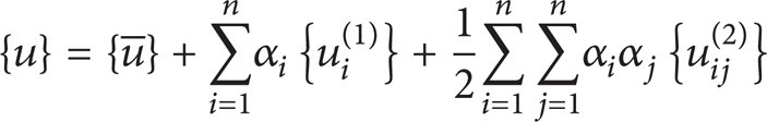
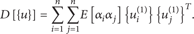
For the governing equation (6), due to the randomness of load or structure, the displacement and stress were random. Therefore, the displacement and stress were expressed as second-order perturbation expressions. The second-order perturbation expressions of displacement were shown in (15). The first moment and second moment of ${u}$ were as follows:

\begin{matrix} E [{u}] = {\bar{u}} + \sum_{i = 1}^{n} E [α_{i}] {u_{i}^{(1)}} + \frac{1}{2} \sum_{i = 1}^{n} \sum_{j = 1}^{n} E [α_{i} α_{j}] {u_{i j}^{(2)}} = {\bar{u}} + \frac{1}{2} \sum_{i = 1}^{n} \sum_{j = 1}^{n} E [α_{i} α_{j}] {u_{i j}^{(2)}}, \\ D [{u}] = \sum_{i = 1}^{n} \sum_{j = 1}^{n} E [α_{i} α_{j}] {u_{i}^{(1)}} {u_{j}^{(1)}}^{T} + \sum_{i = 1}^{n} \sum_{j = 1}^{n} \sum_{k = 1}^{n} {u_{i}^{(1)}} {u_{j k}^{(2)}}^{T} \cdot (E [α_{i} α_{j}] - E [α_{i}] E [α_{j} α_{k}]) + \frac{1}{4} \sum_{i = 1}^{n} \sum_{j = 1}^{n} \sum_{k = 1}^{n} \sum_{l = 1}^{n} {u_{i j}^{(2)}} {u_{k l}^{(2)}}^{T} \times (E [α_{i} α_{j} α_{k} α_{l}] - E [α_{i} α_{j}] E [α_{k} α_{l}]), \end{matrix}

(16)

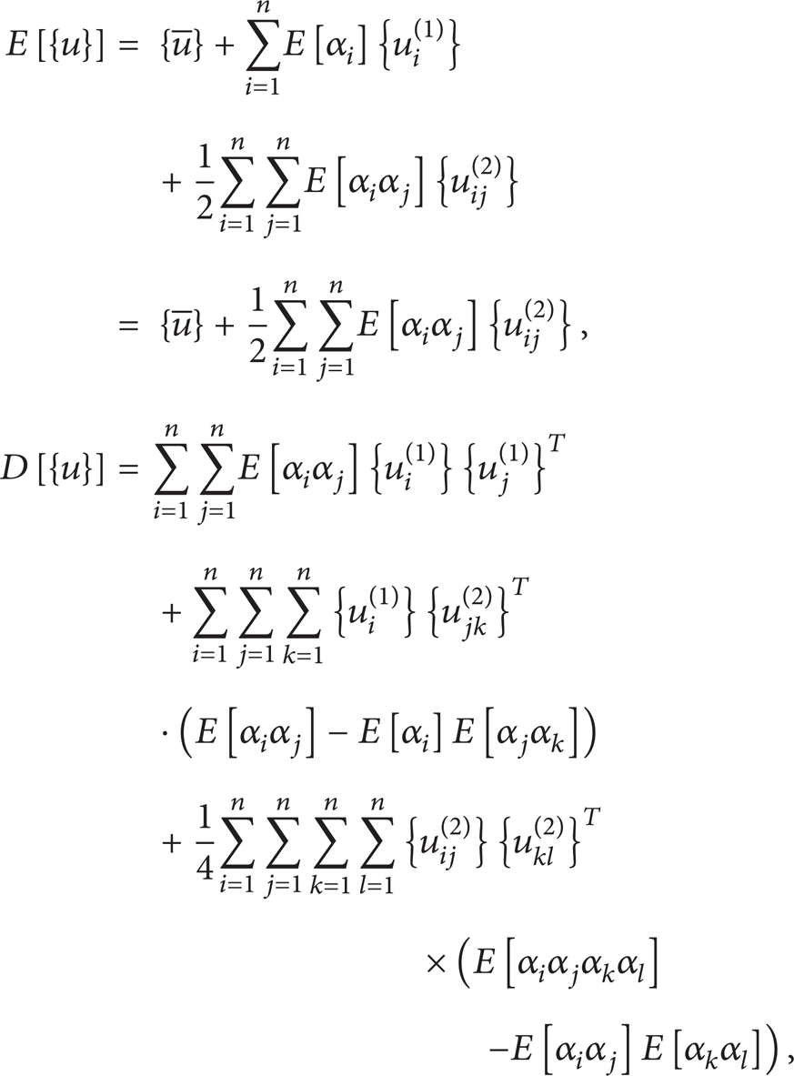
where

E [α_{i} α_{j}] = Cov (Y_{i}, Y_{j}) .

(17)

Generally higher moments of the stochastic field were difficult to obtain and the error was large, so the first item was used as follows:

D [{u}] = \sum_{i = 1}^{n} \sum_{j = 1}^{n} E [α_{i} α_{j}] {u_{i}^{(1)}} {u_{j}^{(1)}}^{T} .

(18)

The second-order perturbation expression of stress was

{σ} = {\bar{σ}} + \sum_{i = 1}^{n} α_{i} {σ_{i}^{(1)}} + \frac{1}{2} \sum_{i = 1}^{n} \sum_{j = 1}^{n} α_{i} α_{j} {σ_{i j}^{(2)}},

(19)

where ${\bar{σ}}$ was the mean value of stress field {σ} at point ${\bar{Y}}$ . {σ_i⁽¹⁾} was the first-order partial derivatives of stress field {σ} on Y_i at point ${\bar{Y}}$ . {σ_ij⁽²⁾} was the second-order partial derivatives of stress field {σ} on Y_i and Y_j at point ${\bar{Y}}$ .

The relationship between stress matrix and strain matrix was

{σ} = [D] {∊} .

(20)

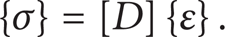
It could be obtained by the perturbation method as follows:

\begin{matrix} {\bar{σ}} = [\bar{D}] {\bar{∊}}, \\ {σ_{i}^{(1)}} = [D_{i}^{(1)}] {\bar{∊}} + [\bar{D}] {∊_{i}^{(1)}}, \\ {σ_{i j}^{(2)}} = [\bar{D}] {∊_{i j}^{(2)}} + [D_{i}^{(1)}] {∊_{j}^{(1)}} + [D_{j}^{(1)}] {∊_{i}^{(1)}} + [D_{i j}^{(2)}] {\bar{∊}} . \end{matrix}

(21)

According to (21), the mean value and variance of stress were

\begin{matrix} E [{σ}] = {\bar{σ}} + \frac{1}{2} \sum_{i = 1}^{n} \sum_{j = 1}^{n} E [α_{i} α_{j}] {σ_{i j}^{(2)}} = [\bar{D}] [B] {\bar{u}} + \frac{1}{2} \sum_{i = 1}^{n} \sum_{j = 1}^{n} E [α_{i} α_{j}] [\bar{D}] [B] {u_{i j}^{(2)}} + [D_{i}^{(1)}] [B] {u_{j}^{(1)}} + [D_{j}^{(1)}] [B] {u_{i}^{(1)}} + [D_{i j}^{(2)}] [B] {\bar{u}}, \\ D [{σ}] = \sum_{i = 1}^{n} \sum_{j = 1}^{n} E [α_{i} α_{j}] {σ_{i}^{(1)}} {σ_{j}^{(1)}}^{T} = \sum_{i = 1}^{n} \sum_{j = 1}^{n} E [α_{i} α_{j}] ([D_{i}^{(1)}] [B] {\bar{u}} + [\bar{D}] [B] {u_{i}^{(1)}}) \cdot {([D_{j}^{(1)}] [B] {\bar{u}} + [\bar{D}] [B] {u_{j}^{(1)}})}^{T} = \sum_{i = 1}^{n} \sum_{j = 1}^{n} E [α_{i} α_{j}] ([S_{i}^{(1)}] [R_{\bar{a} \bar{a}}] {[\bar{S}]}^{T} + [\bar{S}] [R_{a_{i} \bar{a}}] {[S_{i}^{(1)}]}^{T} + [\bar{S}] [R_{a_{i} a_{j}}] {[\bar{S}]}^{T}), \end{matrix}

(22)

where D was elastic matrix and B was strain matrix. We have

\begin{matrix} [S_{i}^{(1)}] = [D_{i}^{(1)}] [B], [\bar{S}] = [\bar{D}] [B], \\ [R_{\bar{a} \bar{a}}] = {\bar{u}} {\bar{u}}^{T}, \\ [R_{a_{i} \bar{a}}] = {[R_{\bar{a} a_{i}}]}^{T} = {\bar{u}} {u_{i}^{(1)}}^{T}, \\ [R_{a_{i} a_{j}}] = {u_{i}^{(1)}} {u_{j}^{(1)}} . \end{matrix}

(23)

It was seen from the derivation that, in order to get the statistical properties of the response, it was necessary to obtain the first-order and second-order partial derivatives of the response to random variables. Explicit algorithm was used in the finite volume method so that the partial derivatives could be solved directly, which was the advantage of the finite volume method for solving stochastic dynamic problems. The partial derivative of (6) to random variable was

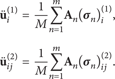
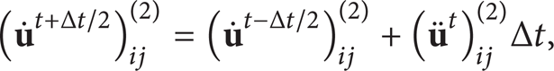
\begin{matrix} {\overset{‥}{u}}_{i}^{(1)} = \frac{1}{M} \sum_{n = 1}^{m} A_{n} {(σ_{n})}_{i}^{(1)}, \\ {\overset{‥}{u}}_{i j}^{(2)} = \frac{1}{M} \sum_{n = 1}^{m} A_{n} {(σ_{n})}_{i j}^{(2)} . \end{matrix}

(24)

If the physical quantities at time t were known, the partial derivatives of displacement at time t + Δt could be obtained by explicit central difference as follows:

{({\dot{u}}^{t + Δ t / 2})}_{i}^{(1)} = {({\dot{u}}^{t - Δ t / 2})}_{i}^{(1)} + {({\overset{‥}{u}}^{t})}_{i}^{(1)} Δ t,

(25)

{(u^{t + Δ t})}_{i}^{(1)} = {(u^{t})}_{i}^{(1)} + {({\dot{u}}^{t + Δ t / 2})}_{i}^{(1)} Δ t,

(26)

{({\dot{u}}^{t + Δ t / 2})}_{i j}^{(2)} = {({\dot{u}}^{t - Δ t / 2})}_{i j}^{(2)} + {({\overset{‥}{u}}^{t})}_{i j}^{(2)} Δ t,

(27)

{(u^{t + Δ t})}_{i j}^{(2)} = {(u^{t})}_{i j}^{(2)} + {({\dot{u}}^{t + Δ t / 2})}_{i j}^{(2)} Δ t .

(28)

The partial derivatives of stress could be given according to (26) and (28):

\begin{matrix} {(σ^{t + Δ t})}_{i}^{(1)} = D_{i}^{(1)} B u^{t + Δ t} + D B {(u^{t + Δ t})}_{i}^{(1)}, \\ {(σ^{t + Δ t})}_{i j}^{(2)} = D_{i j}^{(2)} B u^{t + Δ t} + D_{i}^{(1)} B {(u^{t + Δ t})}_{j}^{(1)} + D_{j}^{(1)} B {(u^{t + Δ t})}_{i}^{(1)} + D B {(u^{t + Δ t})}_{i j}^{(2)} . \end{matrix}

(29)

For the perturbation-finite volume method, the boundary conditions were shown in (30) and the initial conditions were shown in (31) as follows.

Boundary conditions are as follows:

\begin{matrix} \frac{\partial σ}{\partial x_{i}} \cdot n = \frac{\bar{X}}{\partial x_{i}}, \\ \frac{\partial u}{\partial x_{i}} = \frac{\partial \bar{u}}{\partial x_{i}}, \\ \frac{\partial^{2} σ}{\partial x_{i} \partial x_{j}} \cdot n = \frac{\partial^{2} \bar{X}}{\partial x_{i} \partial x_{j}}, \\ \frac{\partial^{2} u}{\partial x_{i} \partial x_{j}} = \frac{\partial^{2} \bar{u}}{\partial x_{i} \partial x_{j}} . \end{matrix}

(30)

Initial conditions are as follows:

\begin{matrix} {\frac{\partial u}{\partial x_{i}} |}_{t = 0} = u_{0}, \\ {\frac{\partial^{2} u}{\partial x_{i} \partial x_{j}} |}_{t = 0} = u_{0}, \\ {\frac{\partial \dot{u}}{\partial x_{i}} |}_{t = 0} = {\dot{u}}_{0}, \\ {\frac{\partial^{2} \dot{u}}{\partial x_{i} \partial x_{j}} |}_{t = 0} = {\dot{u}}_{0} . \end{matrix}

(31)

For the boundary conditions of load, the partial derivatives of load to random variables were added to (24). For the boundary conditions of displacement, if a degree of freedom of a node was constrained, the partial derivative of the acceleration was forced to zero at each time step.

4. Examples Analysis

The stochastic dynamic problems for cantilever beam and clamped beam subjected stochastic dynamic load were solved by perturbation-finite volume method. The results were compared with that produced by monte carlo method, which proved the proposed method was correct. To ensure the accuracy of Monte Carlo, according to the law of large numbers, a large number of samples were required to ensure the credibility of the results. Through the results of perturbation-finite volume method, the structural failure probability was estimated, and the value was 44%. The literature [23] recommended that the number of samples should satisfy certain conditions:

N \geq \frac{100}{P_{f}} .

(32)

Therefore, 10000 samples were used in Monte Carlo Method to satisfy the accuracy.

(A) Cantilever Beam. The calculation model of cantilever beam was shown in Figure 2; the parameters of material were shown in Table 1.

Table 1:

The parameters of material.

Density (kg/m³)	Modulus of elasticity (GPa)	Poisson Ratio

7800	210	0.3

Figure 2:

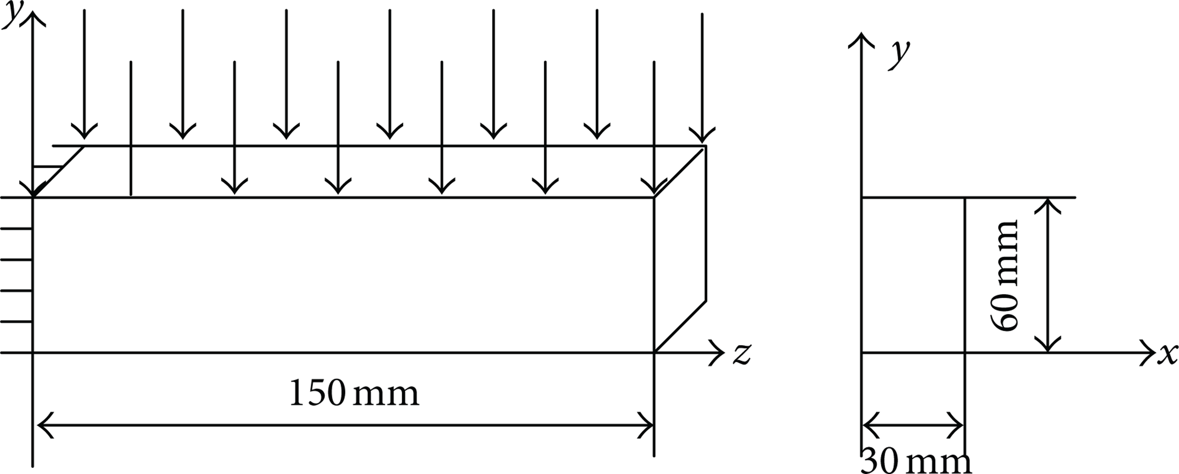
The calculation model of cantilever beam.

The expression of load was

P (t) = P_{m} \exp (- \frac{t}{θ}),

(33)

where

P_{m} = 52.4 {(\frac{w^{1 / 3}}{R})}^{1.13} (MPa), (3.4 MPa < P_{m} < 138 MPa),

(34)

θ = 0.048 w^{1 / 3} {(\frac{w^{1 / 3}}{R})}^{- 0.23} (ms) .

(35)

Here, w and R were the independent random variables. The statistical characteristics of random variables were shown in Table 2.

Table 2:

Statistical characteristics of random variables.

Random variables	Distribution	Mean value	Coefficient of variation

w (kg)	Normal distribution	200.0	0.20
R (m)	Normal distribution	50.0	0.20

The comparison charts of the two methods were shown in Figures 3, 4, 5, and 6.

Figure 3:

Mean value of displacement on node (0.03, 0.06, 0.1) m on direction y.

Figure 4:

Variance of displacement on node (0.03, 0.06, 0.1) m on direction y.

Figure 5:

Mean value of equivalent stress on node (0.03, 0.06, 0.0) m.

Figure 6:

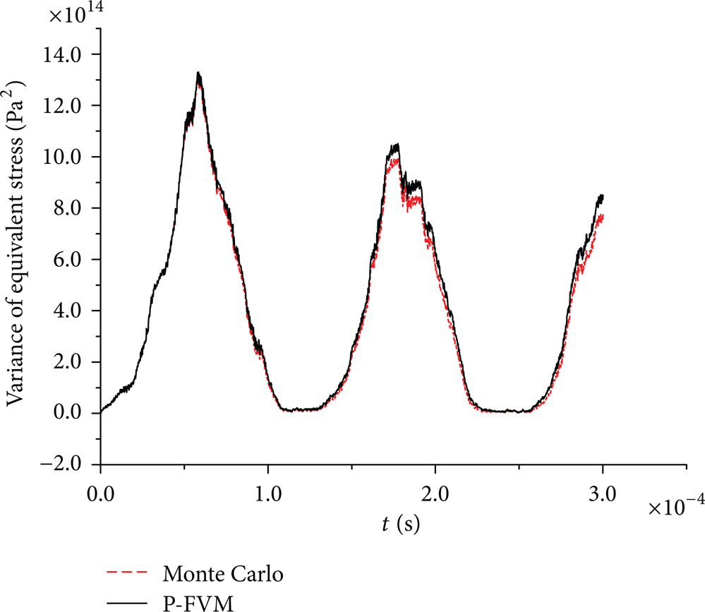
Variance of equivalent stress on node (0.03, 0.06, 0.0) m.

(B) Clamped Beam. The basic parameters of loads and materials were the same as example A (Figure 7), and then the comparison charts of the two methods were shown in Figures 8, 9, 10, and 11.

Figure 7:

The calculation model of clamped beam.

Figure 8:

Mean value of displacement on node (0.03, 0.06, 0.1) m on direction y.

Figure 9:

Variance of displacement on node (0.03, 0.06, 0.1) m on direction y.

Figure 10:

Mean value of equivalent stress on node (0.03, 0.06, 0.0) m.

Figure 11:

Variance of equivalent stress on node (0.03, 0.06, 0.0) m.

From the results of the two examples, it showed that the results of two methods were basically the same, and the calculation accuracy was verified. It has be seen from the comparison of the two methods that the mean value of the displacement and stress fitted better, while the variance of displacement and stress produced a small error in a certain period of time. It was because the mean value of the results was second-order accuracy, the variance was first-order accuracy. It was difficult to obtain the higher moments of stochastic field and the error was large, so only the first term was taken, which leads to a lower calculation accuracy. It needed to be improved in the future. Finally, the correctness of perturbation-finite volume method has been proved by the examples.

(C) The Randomness of Structure and Load. The randomness of structure and load was considered in this example. The calculation model was shown in Figure 2. The density of material was 7800 kg/m³, and the Poisson Ratio was 0.3. The expression of load was the same as (33)–(35), but R was constant and its value was 50 m in this example. Here w and E, structural Modulus of elasticity, were the independent random variables. The statistical characteristics of random variables were shown in Table 3.

Table 3:

Statistical characteristics of random variables.

Random variables	Distribution	Mean value	Coefficient of variation

w (kg)	Normal distribution	200.0	0.20
E (GPa)	Normal distribution	200.0	0.002

The mean value and variance of the responses solved by the Perturbation-Finite Volume Method were shown in Figures 12, 13, 14, and 15.

Figure 12:

Mean value of displacement on node (0.03, 0.06, 0.1) m on direction y.

Figure 13:

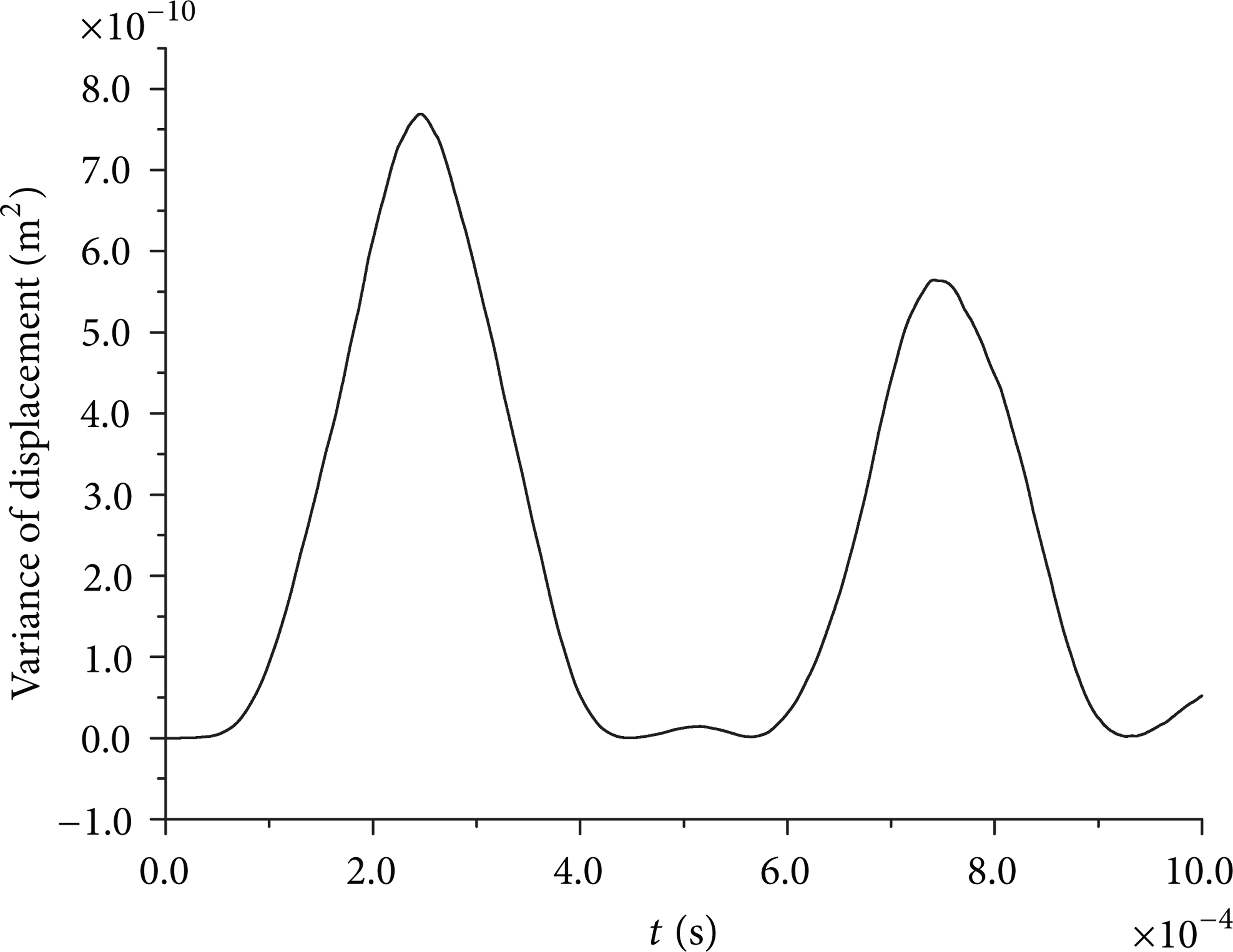
Variance of displacement on node (0.03, 0.06, 0.1) m on direction y.

Figure 14:

Mean value of equivalent stress on node (0.03, 0.06, 0.0) m.

Figure 15:

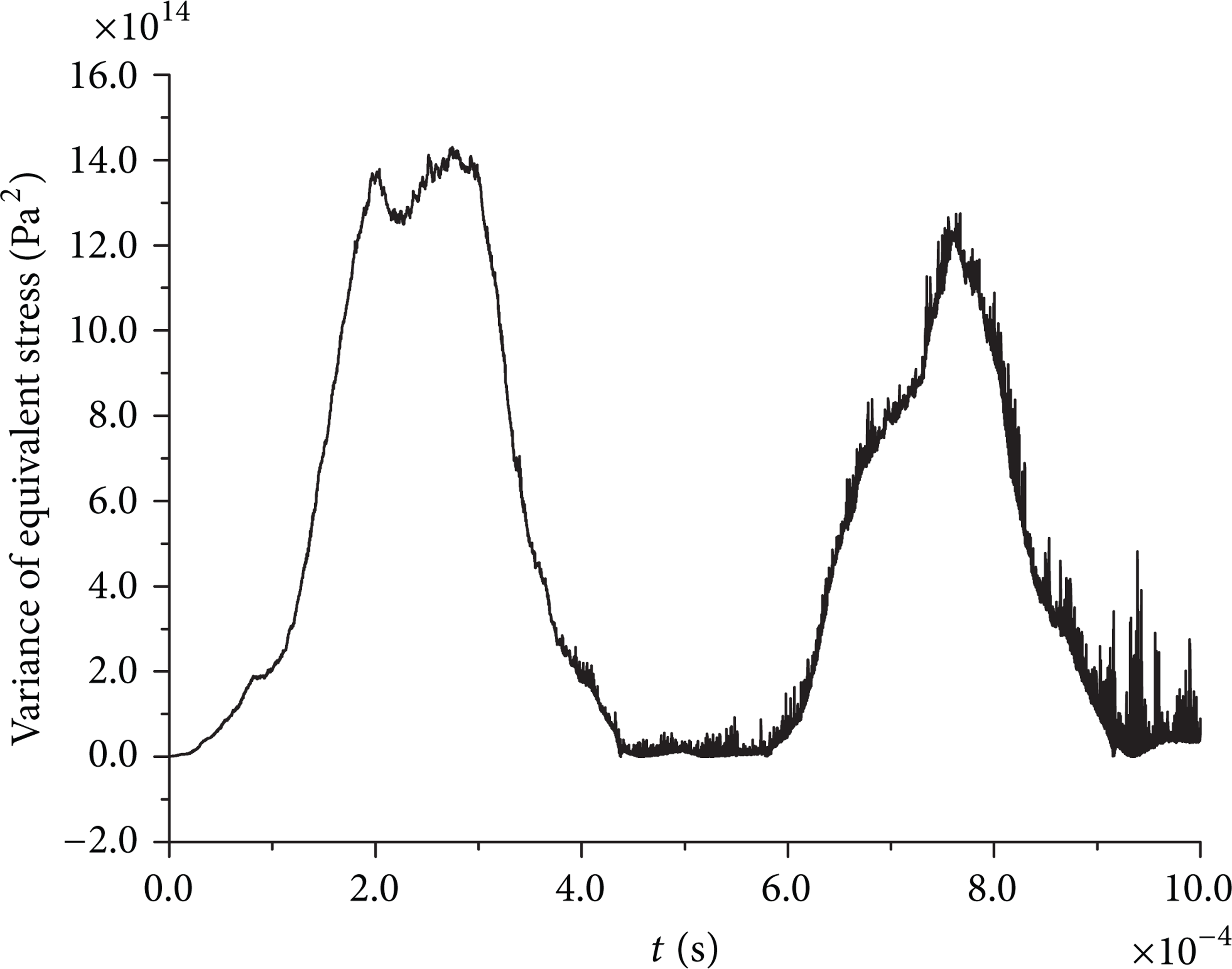
Variance of equivalent stress on node (0.03, 0.06, 0.0) m.

(D) The Stochastic Dynamic Analysis of Linear Multibody System. The perturbation-finite volume method was successfully applied in the stochastic dynamic analysis of linear multibody system, which was verified by the next example. The calculation model of linear multibody system was shown in Figure 16. The sections of copper and steel were the same.

Figure 16:

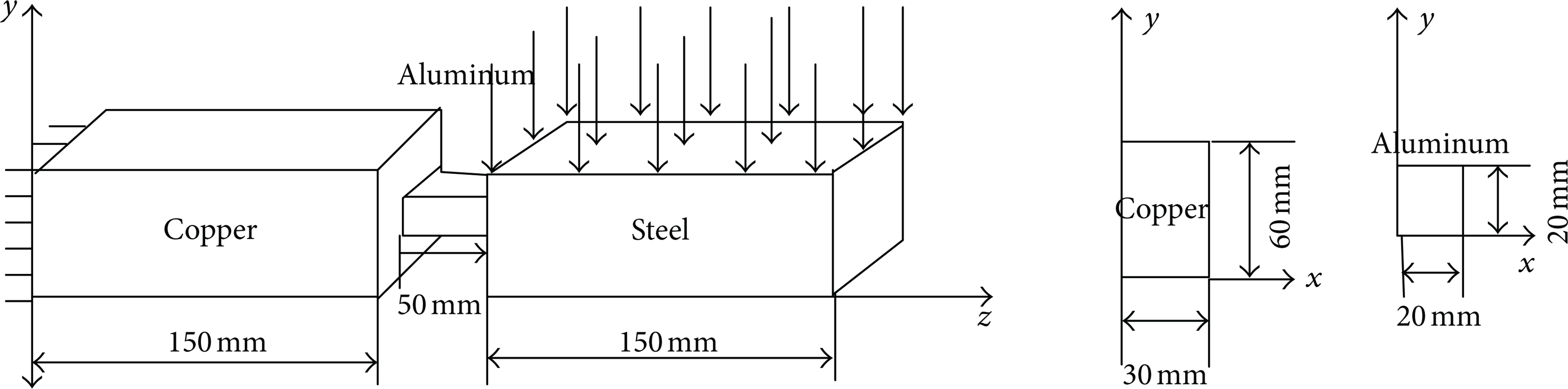
The calculation model of linear multibody system.

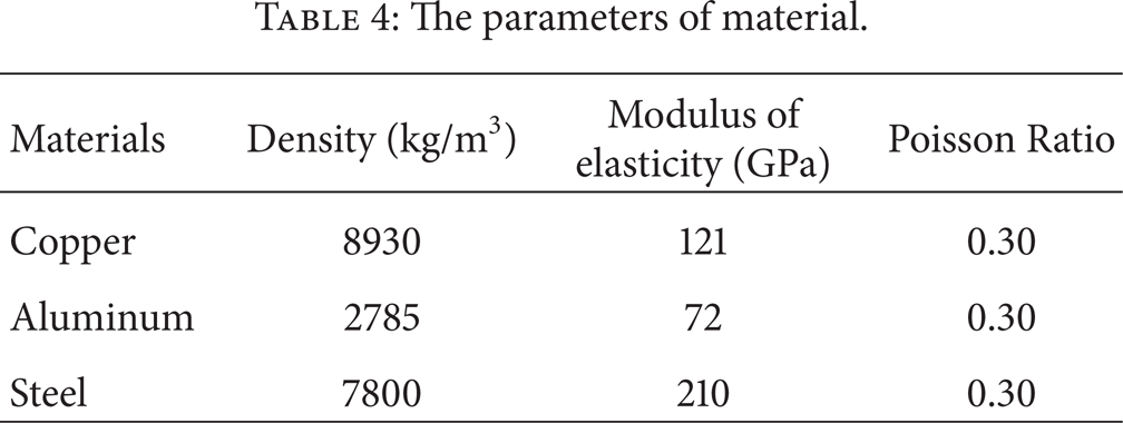
The parameters of materials were shown in Table 4.

Table 4:

The parameters of material.

Materials	Density (kg/m³)	Modulus of elasticity (GPa)	Poisson Ratio

Copper	8930	121	0.30
Aluminum	2785	72	0.30
Steel	7800	210	0.30

The load and the statistical characteristics of random variables were the same as example A. The mean value and variance of the responses solved by the perturbation-finite volume method were shown in Figures 17, 18, 19, and 20.

Figure 17:

Mean value of displacement on node (0.0, 0.06, 0.35) m on direction y.

Figure 18:

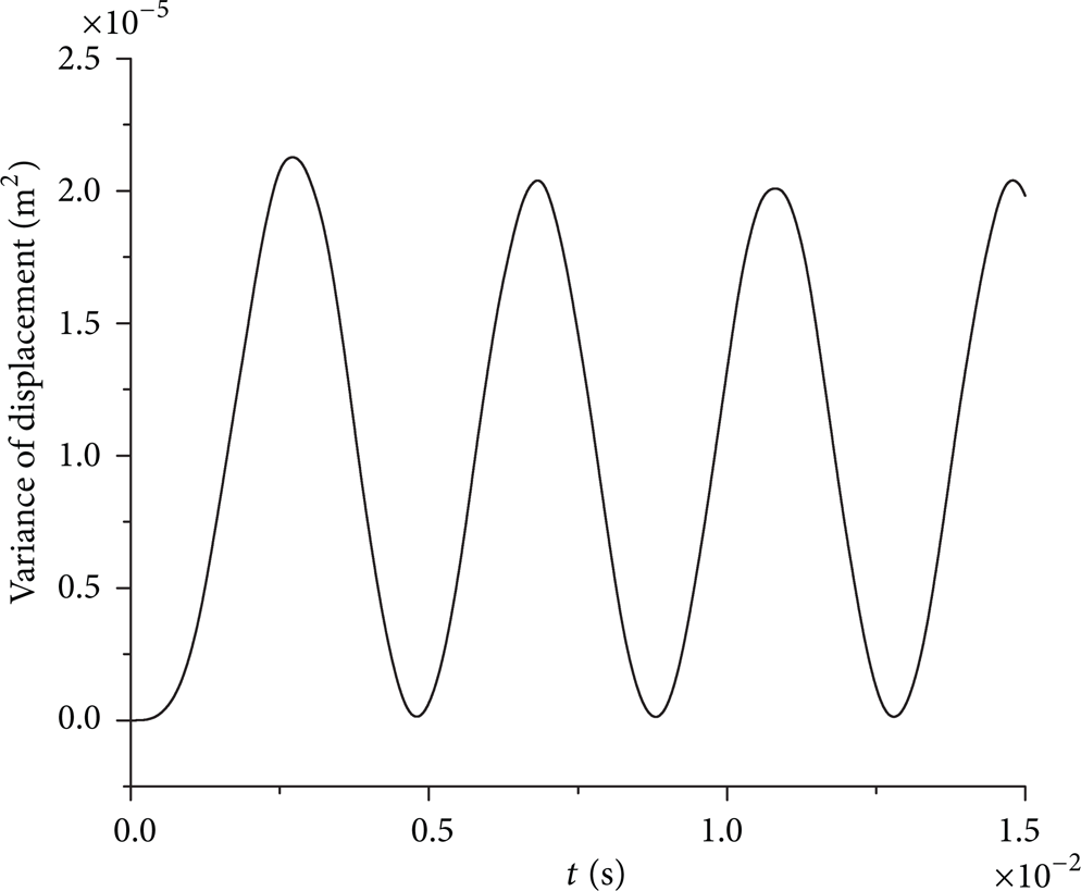
Variance of displacement on node (0.0, 0.06, 0.35) m on direction y.

Figure 19:

Mean value of equivalent stress on node (0.0, 0.058, 0.213) m.

Figure 20:

Variance of equivalent stress on node (0.0, 0.058, 0.213) m.

5. Conclusions

The examples were presented to verify the perturbation-finite volume method. The results of perturbation-finite volume method were compared with the results of Monte Carlo method, which proved that the proposed method was correct and accurate. Therefore, the proposed method was reasonable and effective. This method, theoretically, can be applied to problems under any forms of random dynamic loads. Meanwhile, the perturbation-finite volume Method was successfully applied to the stochastic dynamic analysis of linear multibody system, which was verified by the example D. A new method has been provided for the stochastic dynamic analysis, and it has laid the foundation for the reliability analysis of dynamics.

The benefit of the finite volume method was that the explicit expressions between random response and basic random variables could be given, which greatly reduced the difficulty of stochastic dynamic analysis. It provided some theoretical references for engineering applications. However, this method has something to be improved yet. For example, in the process of calculation, the grid stress was assumed to be constant, which required a small grid to satisfy the accuracy; it restricted the size of components. So, the development of high-precision grid needed to be studied strongly, and the accuracy of the variance of the response should be improved in the future because of the low accuracy.

Footnotes

Acknowledgment

This work was supported by the Science and Technology on Combustion and Explosion Laboratory Foundation (9140C350406150C35126).

References

Chen

and Liu

, Stochastic Finite Element Method and Engineering Application, Southwest Jiaotong University Press, Chengdu, China, 1993.

Zhu

, and Yan

, “Application of stochastic finite element method to analysis of uncertainties,” Journal of Harbin Engineering University, vol. 23, no. 1, pp. 132–135, 2002.

Cui

and Wen

, “Stochastic FEM and its applications in engineering,” Journal of Nanjing University of Aeronautics & Astronautics, vol. 32, no. 1, pp. 91–98, 2000.

Yan

X.-C.

and Hua

, “Structural system reliability analysis based on stochastic finite element method,” Journal of Wuhan University of Technology, vol. 32, no. 9, pp. 69–75, 2010.

Rong

and Lin

, “Reliability analysis for connecting-rod based on SFEM,” Ship Sciences and Technology, vol. 33, no. 9, pp. 68–70, 2011.

Yang

and Li

, “Vectorial cooperative response surface method for stochastic analysis of structures,” Engineering Mechanics, vol. 29, no. 11, pp. 58–64, 2012.

Jing

and Huang

, “Analysis on structure reliability collocation based stochastic finite element method,” Sichuan Building Science, vol. 38, no. 2, pp. 39–41, 2012.

, and Wei

, “Probability and compound uncertainty importance measures of structure stochastic analysis and their computational method,” Chinese Journal of Computational Mechanics, no. 2, pp. 64–71, 2013.

Xiang

Yang

, and Zhao

, “Uncertainty analysis of long-term deformation for prestress concrete beam,” Journal of Civil Architectural & Environmental Engineering, vol. 35, no. 1, pp. 111–116, 2013.

10.

Saltelli

, “Sensitivity analysis for importance assessment,” Risk Analysis, vol. 22, no. 3, pp. 579–590, 2002.

11.

Frey

H. C.

and Patil

S. R.

, “Identification and review of sensitivity analysis methods,” Risk Analysis, vol. 22, no. 3, pp. 553–578, 2002.

12.

Saltelli

Tarantola

, and Campolongo

, “Sensitivity analysis as an ingredient of modeling,” Statistical Science, vol. 15, no. 4, pp. 377–395, 2000.

13.

W.-P.

, “An extended precise integration method for response of a structure subjected to evolutionary random exciation,” Journal of Vibration and Shock, vol. 28, no. 7, pp. 131–142, 2009.

14.

Zhao

Huang

X. Y.

Xia

G. H.

, and Su

X. H.

, “A matrix-free implicit unstructured multigrid finite volume method for simulating structural dynamics and fluid-structure interaction,” Journal of Computational Physics, vol. 225, no. 1, pp. 120–144, 2007.

15.

Chen

J.-B.

and Li

, “Dynamic response and reliability analysis of non-linear stochastic structures,” Probabilistic Engineering Mechanics, vol. 20, no. 1, pp. 33–44, 2005.

16.

Putcha

C. S.

Patev

, and Leggett

M. A.

, “Time-dependent reliability analysis of steel miter gates,” International Journal of Modelling and Simulation, vol. 23, no. 1, pp. 1–12, 2003.

17.

Xiao

Gao

, and Ye

, “Dynamic reliability analysis for structure seismic response based on wavelet,” World Earthquake Engineering, vol. 18, no. 1, pp. 27–33, 2002.

18.

Cao

Lai

, and Bai

, “Estimations of the reliability of structures based on wavelet transform,” World Information on Earthquake Engineering, vol. 16, no. 4, pp. 70–77, 2000.

19.

Qiao

and Lv

, “Dynamic reliability analysis of stochastic structures under non-stationary random excitation,” Chinese Journal of Solid Mechanics, vol. 29, no. 1, pp. 36–40, 2008.

20.

Fallah

, “A cell vertex and cell centred finite volume method for plate bending analysis,” Computer Methods in Applied Mechanics and Engineering, vol. 193, no. 33–35, pp. 3457–3470, 2004.

21.

Xia

and Lin

C.-L.

, “An unstructured finite volume approach for structural dynamics in response to fluid motions,” Computers and Structures, vol. 86, no. 7–8, pp. 684–701, 2008.

22.

Yan

, The Method of Computational Fluid Dynamics and Its Application, Beijing University of Aeronautics and Astronautics Press, Beijing, China, 2003.

23.

Cai

, and Chen

, Reliability Analysis and Optimization Design of Stochastic Structural System, Harbin Engineering University Press, Harbin, China, 2005.

Application of Finite Volume Method to Structural Stochastic Dynamics

Abstract

1. Introduction

2. The Equations of Finite Volume Method

3. The Equations of Perturbation-Finite Volume Method

4. Examples Analysis

5. Conclusions

Footnotes

Acknowledgment

References