A Routing Algorithm Based on Dynamic Forecast of Vehicle Speed and Position in VANET

Abstract

Considering city road environment as the background, by researching GPSR greedy algorithm and the movement characteristics of vehicle nodes in VANET, this paper proposes the concept of circle changing trends angle in vehicle speed fluctuation curve and the movement domain and designs an SWF routing algorithm based on the vehicle speed point forecasted and the changing trends time computation. Simulation experiments are carried out through using a combination of NS-2 and VanetMobiSim software. Compared with the performance of the SWF-GPSR protocol with general GPSR, 2-hop C-GEDIR, and the GRA and AODV protocols, we find that the SWF algorithm has a certain degree of improvement in routing hops, the packet delivery ratio, delay performance, and link stability.

1. Introduction

With the development of mobile communication technology and intelligent transportation technology, even if the drivers do not intervene, any vehicle can participate in collecting and reporting useful traffic information such as section travel time, flow rate, and density, as discussed in [1]. Road conditions, traffic congestion and information can be exchanged between vehicles, including speed, direction, acceleration, and position, which can greatly improve the vehicle safety. Business services (such as infotainment, audio, video, and internet applications) also can be applied in this transportation; in this case, even if people leave the computer and mobile phone, they can sit in the car to get the leisure and entertainment. The realization of these ideas comes from VANET (vehicle ad hoc network technology) in [2].

The VANET vehicles must be equipped with a radio transceiver and computer control module, so that they can be used as a network node. The wireless network coverage range of each vehicle may be limited to a few hundred meters; each node can be either a transceiver or a router. Therefore, it is necessary to provide end-to-end communication over long distances by means of intermediate nodes. The VANET does not need the support of wired infrastructure, but some of the permanent network nodes may appear in the form of a roadside unit. Roadside units can provide a wide variety of vehicle network services, such as the placement of information in the driveway side, providing geographic data information, or using buses, taxis, and other vehicles as a gateway to connect to internet as discussed in [3].

Ad hoc network is a kind of distributed wireless multihop network composed of a group of nodes with routing function, and it does not rely on any of the default network infrastructures. In ad hoc network, the transmission range of nodes is limited. When the source node sends data to the target node, it usually requires other auxiliary node, so routing protocol is an indispensable part of the ad hoc network as discussed in [4]. Traditional data aggregation schemes for wireless sensor networks usually rely on a fixed routing structure to ensure that data can be aggregated at certain sensor nodes. However, they cannot be applied in highly mobile vehicular environments. Unlike the traditional ad hoc networks [5], VANET has some different characteristics such as regularity and predictability [6]. The global positioning system (GPS) can provide precise positioning service for vehicles. However vehicle is moving at high speed, obstruction in existence, and frequent changes in network topology, so VANET routing leads to more complex routing problems. From a functional perspective, the routing protocol is a mechanism by which communication network sets guidelines for the business data from the source node to the destination node. The design objectives of routing protocol are to meet the application requirements while minimizing the network energy consumption, to use resources effectively, and to expand the network throughput. Among them, the application's needs generally include delay, delay jitter, and packet loss rate. And the network capacity can be seen as a function, which is related to each node's available resources, the number of nodes in the network, node density, the end-to-end communication frequency and topology changes, and other factors, as discussed in [7]. VANET routing protocols have three common classifications: greedy perimeter stateless routing (GPSR) routing algorithm is an algorithm using location information routing, which uses a greedy algorithm to establish the routing in [8]. As discussed in [9], resource-constrained mobile sensors require periodic position measurements for navigation around the sensing region.

2. Problem Statement

GPSR protocol is a stateless routing protocol and a typical location-based routing protocol; it requires neither regular exchange of routing information nor broadcast flooding to route requests. And it does not need to store routing information, thus reducing the network bandwidth resource consumption and the processing power of node, which is very effective in a network for high density and node average distribution, such as a highway. But in recent years, many researchers have found that implementation of GPSR in the city road environment leads to some defects as the following aspects.

2.1. The Unstable Link and a Huge Amount of Computation

The GPSR protocol uses greedy forwarding strategy, selecting the nearest neighbor node from the destination node as the next hop node in the network, which means that it is the farthest from neighbor nodes to the local node, so the link is unstable in a large probability. Because of the frequent movement of node in the network, the speed of the vehicle will result in changes of the distance between the nodes. Also the greedy algorithm cannot be effectively computed, so the unstable link will lead to decline in the performance of the protocol. Changing topology makes the computation of the greedy algorithm large, but the computing power and energy of node is limited; in this case, GPSR protocol needs flattening to eliminate the cross-links in the network topology, so when each node adds or deletes any one of its neighbor nodes, it requires to flatten the local topology. The time complexity of this process is $(n^2)$ , in which n is the density of the node's neighbors. When the network topology changes frequently, this problem will become more serious.

For example, source node is X, and the destination node is Y. If, at a time $T_0$ , the node  X  needs to send data packet to the node Y, and node X knows the location of the node Y at this time, then according to the GPSR protocol, the source node and the intermediate node can transmit directly packet forwarding based on position information of the destination node at that moment. However, the destination node is moving in the actual scene, and the intermediate node is likely to transmit packet forwarding to the destination node which has moved to another position based on the position information of the destination node at the time   $T_0$ . Then to route addressing continues, an error may occur. It is likely that the data packet arrives at the position of the destination node in the time   $T_0$ . If the surrounding node has no position information of the destination node, then the data packet cannot be transmitted to the destination node, which means packet forwarding failure; in other words, packet will be lost.

2.2. Packet Loss and the Increase in the Number of Routing Hops

The greedy forwarding policy and boundary forwarding strategy of the GPSR protocol will lead to redundancy problem. The uneven distribution of the nodes in a city environment will lead to network congestion and packet loss when the load of network is too large, and the wrong greedy forwarding will take up too much resources. The GPSR algorithm uses the right hand to search routes at the boundary in a direction; it may choose relatively long routing paths to reach the destination node, even nearer routing path in the other direction exists. In fact, when the density of network nodes increases, the boundary forwarding policy leading to routing hops increases, resulting in waste of the channel resources as well as the increase in network delay. When the distribution of network nodes is sparse, because of the use of unified right-hand rule, a message in a boundary mode is likely to repeatedly miss the opportunity to change back to the greedy forwarding mode, which needs to go through a lot of mode nodes.

For example, because of the limitations of the cruciform road topology, node distribution is very uneven. The source node X needs to select a node Y as the next hop node; if the node Y is the best host, then it is transferred to the boundary forwarding mode. Then implementing the right-hand rule, there will be two results: one is that packet will eventually arrive at the destination node, but the results of this addressing increased routing hops; another is that there is large number of nodes on the left side of the node Y, then the packet may have been sent along the left hand side of the road to go farther and farther away from the target until life cycle of the last node is reduced to 0, and then discard the packet.

3. The Algorithm Design

3.1. Relative Speed Fluctuation and Distance Change between Nodes

Real-time computing needs to constantly recalculate the route for change of dynamic speed, which brings about enormous computation. Due to high-speed mobility of node, speed is roughly between 5~40 m/s, resulting in rapid changes in the network topology, so the life of path is short. For example, the average speed is 100 km/h on the road; if the node's coverage radius is 250 m, then the probability of the persistent link exists for 15s is only 57%, as discussed in [10]. In [11], with the knowledge of the access point locations, more accurate localization for the mobile device trajectories and motion sensors can be obtained. In [12], bounding-box mechanism is a well-known low-cost localization approach for wireless sensor networks. However, the bounding-box location information cannot distinguish the relative locations of neighboring sensors.

Therefore, before the route discovery, forecast of the relativly more stable links is important. The vehicle nodes with relativly more stable speed and trajectory can improve the efficiency of the greedy algorithm and reduce the computational energy consumption. The greedy algorithm selects the nearest node from the target node to send forwards. However, because the vehicle is in a state of movement or stoppage at any time, the speed of the node is changing, so the distance between the nodes is also changed. According to the research, for a car traveling in the big city, the average speed is about 30 km/h, depending on traffic conditions. In general, the limit of maximum speed is 60 km/h on urban trunk road, is 40 km/h on urban secondary roads, and is 30 to 40 km/h in ramp and tunnel is. There are two major possibilities about the vehicle speed changes, one is road congestion, and the other is wait for traffic lights or parking in intersection. In either case, we can consider only the relative velocity between the vehicle nodes. If the speed of nodes is the same or vehicles park simultaneously at the same time, the relative speed is 0. In [13], the difference in propagation speed helps to report encounters between nodes. Therefore, if the vehicle is accelerating or decelerating, the relative speed increases or decreases, the distance between nodes changes, then the shortest path between the nodes also changes.

If the relative speed of the vehicles between nodes is greater than the speed threshold value   $V_z$ , forwarding node may exceed the signal radiation range of the source node in the time threshold   $T_z$ ; the packet should be considered to be sent to another one. However, the speed of the vehicle is unpredictable; we will design a heuristic algorithm to forecast the speed fluctuation to predict the movement of the vehicle. Some improved GPSR routing protocol will take into account the direction of movement of the vehicle. Reference [14] proposed a mobile target tracking scheme that takes full advantage of Voronoi diagram boundary to improve detection ability. In fact, no matter vehicles traveling to the same direction or opposite, and the vehicles are in front or behind of each other, they cannot affect the distance between nodes in greedy routing algorithm if we can predict and compute the relative speed of vehicles. The method can also forecast multiple nodes within a topology; if the majority of nodes of the entire topology are in a stable state of relative speed, the problems caused by the network topology changing too quickly can be improved to some extent.

For example, in the time of $t_{(x)}$ , the speed points forecasted of source node A were 20, 23, 25, 15, and 10 m/s, the speed points forecasted of forwarding node B car were 23, 21, 20, 18, and 19 m/s, and then the relative speed of the two vehicles were 3, 2, 5, 3,  and 9 m/s, whereas the relative distance were   ${3t}_{(1)}$ , ${2t}_{(2)}$ , ${5t}_{(3)}$ , ${3t}_{(4)}$ , and ${9t}_{(5)}$  m. If the relative distance was more than communication circle radius R of A, A cannot communicate with B at this moment. If within the time threshold $T_z$ , A was unable to send data packet to B, the relative speeds was unstable; consider giving up point B from routing. Conversely, within the time threshold value $T_z$ , the forecast result of the relative speed leading to the distances between B and A was less than R; it can be considered that the node B relative to A was stable and can be used as the next hop of the routing. If there were multiple stable nodes or no stable node, implement greedy forwarding directly. The change in distance caused by speed fluctuated as shown in Figure 1.

Figure 1

The change in distance caused by speed fluctuation.

3.2. Ideal and Optimal Forwarding Nodes and Movement Domain

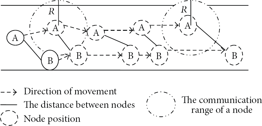
In [15], the resultant formulation of the DGPR (distributed Gaussian process regression) approach only requires neighbor-to-neighbor communication, which enables each sensor node within a network to produce the regression result independently. When node A found the next forwarding node B, B node was located the boundary of the circle the radius was R of communication range of A; we considered that B was optimal forwarding node of A. Similarly, if C was the optimal forwarding node of B, D was optimal forwarding node of C; we considered this particular routing to be called continuous ideal and optimal routing, which was the shortest distance routing at this time.

As discussed in [16], localization is one of the most important issues in wireless sensor networks. But no orderliness for locations of nodes changes at any time when vehicles travel on the road. The emergence of continuous ideal and optimal routing was unlikely. But the possibility of the approximate continuous ideal and optimal routing is there. When there was the closest distance between the target node and B, which was infinitely closed to communication circle radius R of A, we can take the point B as the approximate optimal forwarding node. If the infinitely close to ideal and optimal forwarding nodes in the process of forwarding information can be computed, the number of routing hops can be declined. However, since the vehicle is traveling without the law can be followed, we designed a motion range computation method, used to predict the movement trajectory of the vehicles. In the VANET, mobile nodes are subjected to the restrictions of the road models. Although it is not possible to accurately compute the position of the destination node at a particular moment, it can estimate the range of its movement. Reference [17] presents a novel probabilistic framework for reliable indoor positioning of mobile sensor network devices. As discussed by LAR protocol, the source node X is assumed to know that the position of the destination node D is $L(X_x,Y_y)$   at this moment, and the average moving speed is $V_p$ . Therefore the region where the node D may occur can be estimated. The region is the circular region which used $L(X_x,Y_y)$ as the center,   $R=V_p\times (T_1-T_0)$   as the radius. It is the “desired domain.” However, the error may be very serious which uses average speed to compute the mobile range of vehicles.

When implementing speed ​ ​fluctuation forecasted to predict the curve of the speed, distance between the node A and B can be computed at $t_{(x)}$ time. However, the vehicle traveling on the road does not necessarily move straight. In fact, in most of the cases, the vehicles are doing the curvilinear motion. So directly compute the straight-line distance between the two nodes that will certainly cause serious errors. Therefore, if the position coordinates of the A and B were A $(x_{\text{A}},y_{\text{A}})$ and B $(x_{\text{B}},y_{\text{B}})$ , when $x_{\text{A}}=x_{\text{B}}$ , then the positions of A and B were on back and forth of a straight line; the straight line distance can be computed; if $y_{\text{A}}=y_{\text{B}}$ , A and B located on the road around the location and straight-line distance can also be computed. Since communication range of a single hop node is only a few hundred meters in [18], the width of the urban road W is typically much less than the signal transmission range of vehicle node. When $y_{\text{A}}=y_{\text{B}}$ , it is possible to compute its distance, because the greedy algorithm should select the node from which to the source node is the farthest away. If $x_{\text{A}}=x_{\text{B}}$ , the distance K should be computed; K-value is the closer to the optimal node, the possibility of which is the forwarding nodes is great. Therefore, the average speed $V_p$ cannot make the diameter $2R$ of the desired domain exceed the road width W; if the diameter is longer than the width, the maximum speed $V_t$ in the curve should be loop selected to compute until $2R=2V_p\times (T_1-T_0)\le W$ ; the array of speed will achieve stability and convergence. The packet forwarding of original GPSR protocol is based on the position information of the destination node; the node is no longer forwarding the packet to a fixed position coordinates, but to the region where the destination node may occur, that is, forwarding the packet to a moving area; we call it “movement domain.”

The localization problem in mobile sensor networks is a challenging task, especially when measurements exchanged between sensors may contain outliers, that is, data not matching the observation model in [19]. If the continuous ideal and optimal routing exist in the case, the signal packet transmission speed was $V_x$ between the four nodes: A, B, C, and D, the radius of signal transmission circle was $R_x$ , and the time of A sending the data to the D directly was $R_{\text{A}}/V_{\text{A}}+R_{\text{B}}/V_{\text{B}}+R_{\text{C}}/V_{\text{C}}+R_{\text{D}}/V_{\text{D}}$ . Based on the speed fluctuations forecasted algorithm, in that period of time, we have to select the speed point forecast: $V_{\text{A}}$ , $V_{\text{B}}$ , $V_{\text{C}}$ , and $V_{\text{D}}$ , the distance is the shortest among the four nodes, the instant speed of four nodes was selected from the speed forecasted queue. The optimal forwarding nodes and node movement domain as shown in Figure 2. As shown above, the vehicle is not a linear movement, select the speed forecasted to compute movement domain of nodes, we can predict the range of movement of the vehicles. Therefore, if traffic is heavy, when signal packet transmission range of the vehicle is greater than the distance between nodes, the packet can be directly forwarded to the location of the movement domain. If there is less traffic on the road, the distance between nodes may be greater than the diameter of signal packet transmission circle, which may result in the inability to send the data. At this time, the greedy algorithm can use border forwarding to search forward node.

Figure 2

The optimal forwarding nodes and node movement domain.

3.3. SWF Routing Algorithm

The basic principles of GPSR greedy forwarding algorithm are when the node is in greedy forwarding mode, source node select nodes of the farthest distance from themselves within communication range, which is the nearest to the destination node as the next hop node. As discussed in [20], select the node nearest to the destination node as a relay node within the transmission range so that to increase the possibility of a local maximum and link loss because of high mobility and urban road characteristics. So, we design a kind of SWF (Speed Wave Forecasted) routing algorithm combined with speed fluctuation forecasted and computation of the movement domain, as the speed fluctuations forecasted algorithm needs to input the data of speed fluctuations of the vehicle. The vehicle begins to move, to start route discovery, first greedy forwarding. Begin to forecast the speed of the vehicle which is computed at the time threshold value $T_Q$ . Because the possibility of movement changes of the stable relative speed of nodes is small, so put them in a routing node queue and implement greedy forwarding. At the same time, compute distance of approximate ideal and optimal nodes and movement domain. If the distance between movement domains of nodes is smaller than greedy forwarding distance between nodes, then select the approximate ideal and optimal node as forwarding node. Conversely, the greedy algorithm will select the node which is the nearest from target node as forwarding node. When there is a problem of routing void, not implementing boundary forwarding at once, but waiting storage for the time T, waiting for the forwarding node P reaches the mobile domain; if it arrives, it is forwarded to the P, then continue to greedy forwarding, or into the border mode. When the nodes are into the border forwarding mode, if there are no neighbor nodes which are closer from the movement domain of the destination node than their own, so construct flat graph, using the right-hand rule, and find the closest to the movement domain within the transmission range of the node as the next hop node. Until the border forwarding is finished, return to the greedy forwarding.

3.4. Speed Fluctuations Forecasted Algorithm

Assuming GPS is installed in each vehicle, vehicles can determine their own location information. Electronic map can provide the actual road information in each of the navigation system. Determine the travel path of the vehicle before departure from automatic GPS navigation. For a car traveling in the city roads, the speed change can be seen as a volatile process. Whenever vehicles's continuous acceleration last time n, then the speed is bound to enter a downward spiral. Its decline is due to aforementioned road congestion, traffic lights, speed limits, and other objective factors. Conversely, when the vehicle speed reaches the lowest point, wave of continuous acceleration fluctuations also occur; when the fluctuations reach the steady state, if the continuous distribution time K of the speed can be forecasted, we can know the relative speed between the vehicles; it can be found as a relatively stable routing and associated collection of nodes.

Definition 1.

Due to more attributes impacting velocity fluctuations, we set up the N tuple: $〈V_{\lim },M,\text{B}\dots 〉$ with an uncertain definition, among which $V_{\lim }$ is the maximum speed of the vehicle, M is road congestion, and B is probability of randomly moving. In a curve graph showing speed trend fluctuations, the velocity curve as a circular is divided into aliquots n. According to the fluctuation of curves, the change in angle of the waves can be found and is called circle changing trends angle, in order to compute the time of continuous and stable vehicles speed last out, which is Speed fluctuations changing trends time. Set speed trend wave forecasted as (I, I, II, II, III, IV, V, VI, VII…); time balance point of trend wave as the value of X-axis, its identification symbol is $X_T$ , X belongs to W; speed balance point of trend wave as the value of Y-axis, its identification symbol is s.

3.5. Speed Point Forecasted of the Speed Trend Wave

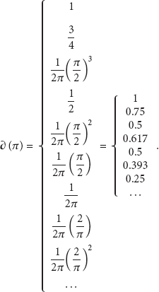
As discussed in [21], a number of routing protocols have been developed in the last years based on SI principles, and, more specifically, taking inspiration from foraging behaviors of ant and bee colonies. The idea of speed forecasted comes from the wave fluctuations in equilibrium theory in [22]; when the continuous decline of the I wave speed is complete, the number of speed point forecasted of the increase wave II is usually π times of wave I; the very small number of cases may exceed π times. Top speed of vehicle node on road of the first wave change of velocity is 20 m/s; the minimum speed is 5 m/s. When II = III, top speed of wave II is s (II) = 62.8 m/s; minimum speed is about 15.7 m/s. $\text{I}/\mathrm{2}=(\mathrm{2}/\mathrm{2}\pi )\times \text{II}$ , use   $\pi /\mathrm{2}$   as a constant, can compute several other possible speed points of waves II. The   $\pi /\mathrm{2}$   times of midpoint of wave I is a speed point forecasted X, as $(\mathrm{1}/\mathrm{2})\text{I}\times (\pi /\mathrm{2})=(\mathrm{1}/\mathrm{2}\pi )\times (\pi /\mathrm{2})\text{II}=(\mathrm{1}/\mathrm{4})\text{II}$ ;    $\pi /\mathrm{2}$   times of X point; is the next speed point forecasted Y; as $(\mathrm{1}/\mathrm{4})\text{II}\times (\pi /\mathrm{2})=(\pi /\mathrm{8})\text{II}=\mathrm{0.393}\text{II}$ . The $\pi /\mathrm{2}$ times of Y point is the next speed point forecasted Z, as $(\pi /\mathrm{8})\text{II}\times (\pi /\mathrm{2})=({\pi }^{\mathrm{2}}/\mathrm{16})\text{II}=\mathrm{0.617}\text{II}$ , use   $\partial (\pi )$   to express the division ratio of the group speed waves. Similarly, use $\pi /\mathrm{2}$ as a constant rate to partition wave I, also calculate speed point forecasted of the wave I. According to the speed partition rate calculation method, use   $\pi /\mathrm{2}$   ratio partition speed point forecasted waves split below the wave I/2; another group speed points forecasted can be obtained before the speed wave trend change. Merge speed points forecasted partitioned by $\pi /\mathrm{2}$ and $\pi /\mathrm{2}$ , and obtain speed points collection coefficient $\partial (\mathrm{5})$ partitioned by pi and the speed points forecasted as shown in Figure 3.

$$\begin{array}{cc}& \partial \left(\pi \right)=\{\begin{array}{c}1\\ \frac{3}{4}\\ \frac{\mathrm{1}}{\mathrm{2}\pi }{\left(\frac{\pi }{\mathrm{2}}\right)}^{\mathrm{3}}\\ \frac{\mathrm{1}}{\mathrm{2}}\\ \frac{\mathrm{1}}{\mathrm{2}\pi }{\left(\frac{\pi }{\mathrm{2}}\right)}^{\mathrm{2}}\\ \frac{\mathrm{1}}{\mathrm{2}\pi }\left(\frac{\pi }{\mathrm{2}}\right)\\ \frac{\mathrm{1}}{\mathrm{2}\pi }\\ \frac{\mathrm{1}}{\mathrm{2}\pi }\left(\frac{\mathrm{2}}{\pi }\right)\\ \frac{\mathrm{1}}{\mathrm{2}\pi }{\left(\frac{\mathrm{2}}{\pi }\right)}^{\mathrm{2}}\\ \dots \end{array}=\{\begin{array}{c}1\\ 0.75\\ 0.5\\ 0.617\\ 0.5\\ 0.393\\ 0.25\\ \dots \end{array}.\end{array}$$

(1)

Figure 3

Speed points forecasted.

The heuristic formula of speed points forecasted of wave II can be summed up:

$$\begin{array}{cc}& s\left(t\right)=\partial \left(\pi \right)\text{II}=\frac{\mathrm{2}}{\pi }\pi \text{I}.\end{array}$$

(2)

So we can obtain a set of speed points forecasted: $A=5$  m/s, $Y=7.86$  m/s, and $Z=10$  m/s.

3.6. Speed Fluctuations Changing Trends Time

The time balance line of the vertical direction of the circle is divided into aliquots n that is changing trends time point for wave fluctuations; when wave goes through time balanced line or into the time zone near the balanced line, the fluctuations will changing trends or increase. Set waves I and II running time as 20 seconds, wave III running time is 25 seconds. The change trends angle of aliquots 5 circle is $\partial (\mathrm{5})=({72}^{°},{144}^{°},{216}^{°},{288}^{°},{360}^{°})$ . Let 288° is the closest from waves III running time denote changing trends time point of waves III, is 4/5 times of circle changing trends time; the changing trends time of wave II arriving in the position of wave III is about 16 seconds, so heuristic formula of changing trends time is

$$\begin{array}{cc}& \text{II}{\text{I}}_T=\left({\text{I}}_T+\text{I}{\text{I}}_T\right)\partial \left(n\right).\end{array}$$

(3)

For a wave run 30 seconds for the situation, select the speed of the data transmission node A according to the running speed of the vehicle to input speed values and ​ ​computed. That means input of the values of the points of speed wave I into speed fluctuations forecasted algorithm after 30 seconds through heuristic formula computing speed point forecasted and speed fluctuations changing trends time after wave I emerges. According to formula (3), wave I running lasts 32 seconds, wave II running lasts 28 seconds, then the changing trends time point when the speed wave reach to waves III is 7/10 times of 60 seconds cycle, is 42 seconds, which means that, after about 42 seconds, the vehicle speed will rise, so $({\text{I}}_T+\text{I}{\text{I}}_T)\partial (\mathrm{7})=\mathrm{60}\times \mathrm{7}/\mathrm{10}=\mathrm{42}$ . In summary, the time of the vehicle stable speed is 42 seconds; accelerating wave III appears from 60 seconds to 102 seconds of II wave; vehicles will reach top speed at the time of 102 seconds. Speed fluctuations changing trends time as shown in Figure 4.

Figure 4

Speed fluctuations changing trends time.

4. Simulation Experiments and Evaluation

NS-2 is a discrete event-driven, object-oriented network emulator. Using NS-2 to simulate network transmission through the establishment of a statistical model, for the design and evaluation of network protocols to provide a good experiment and test platform, compare SWF-GPSR with GPSR and other routing protocols. For comparison performance of the forwarding strategies, select three key indicators for evaluating routing protocols for data collection and analysis of results.

• (1)

Average transmission delay: average time of the transmitter sends a complete data packet to the receiving node.

(2)

Packet delivery success rate: ratio of the total number of packets successfully received to the total number of packets sent.

(3)

Route length: the number of nodes through which data packet from the source node to the destination node successfully posted, that is, the count of hop.

(4)

Link stability: the number of routing link changes in simulation time.

In order to improve the shortage of NS-2 for VANET for network simulation, using vehicular ad hoc networks mobility simulator (VanetMobiSim) software for traffic simulation, establish a system simulation model for simulating nodes move, in order to gain traffic reports and other information on traffic engineering analysis. VanetMobiSim arising from CanuMobiSim (communication in ad hoc networks for ubiquitous computing) is a framework for user mobility model which was developed by CANU research group of Stuttgart University based on JAVA language. It not only contains a certain amount of movement model, but also comprises the analyzer of the geographic data of different formats and visualization module, based primarily on the concept of the module that can be inserted, easy to be expanded, and able to support different types of mobile network simulation or simulation tools, such as NS-2, GloMoSim, and QualNet.

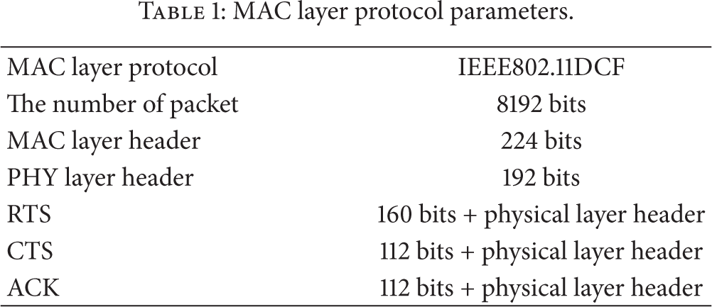
The simulation model map is Manhattan model. In Manhattan model, square grid denotes housing and mesh grid denotes street. The simulation experiments parameters are set as shown in Tables 1, 2, and 3.

Table 1

MAC layer protocol parameters.

MAC layer protocol	IEEE802.11DCF
The number of packet	8192 bits
MAC layer header	224 bits
PHY layer header	192 bits
RTS	160 bits + physical layer header
CTS	112 bits + physical layer header
ACK	112 bits + physical layer header

Table 2

Simulation parameters.

Simulation duration	800 s
Interval of HELLO packet	2 s
Each node can produce data	30 sets
The number of nodes	100
Send packets cycle of CBR (constant bit rate) packets	1 s
Scene area	3500 m × 2500 m (7 × 5 grid, street length is 500 m)

Table 3

Vehicles parameters.

The maximum communication range of car node	300 m
The maximum speed of the vehicle	20 m/s
The minimum speed of the vehicle	5 m/s
Average moving speed	10 m/s
Average residence time when vehicles are at the intersection	2 s
Average maximal distance between vehicles	30 m

In the simulation experiments, we compare SWF-GPSR (GPSR protocol based on SWF algorithm) protocol with general GPSR, 2-hop C-GEDIR, GRA and AODV protocols. Among them, 2-hop C-GEDIR (geographic distance routing) is the GPSR protocol variant, as discussed in [20]. Selecting some of the neighbors to forward the packet, neighbors that received the data packet continue to run the greedy algorithm. Node knows the location information of all it's hop and two-hop neighbor nodes. When a data packet is received, the node selected the nearest node X from the destination point from it's hop and two-hop neighbor nodes. If X is a hop neighbor, then the packet is forwarded directly to the X; if X is two-hop neighbor, it will have to find out neighbor node y to be able to reach X; data packets are submitted to X through y. We can see from Figure 5 that, in urban environment, due to the changing of the topology, the packet forwarding hops increase. Compared with general GPSR and 2-hop C-GEDIR, the number of hops of SWF-GPSR protocol is fewer in the packet forwarding process.

Figure 5

Comparison of average routing hops contrast.

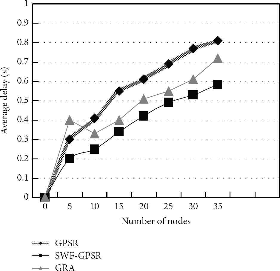
The GRA (geographical routing algorithm) is another variant of GPSR protocol, which is different from GPSR; when local optimization problems occur, GRA will start the route discovery mechanisms (flooding mechanism) to search route to the destination node from the best host. If a route reply message is received, save the route in the routing table to reduce the number of routing lookup process that may occur in the future. As can be seen from Figure 6, in the urban road environment, with the increase of the number of nodes, the gap of average delay end-to-end between general GPSR and SWF-GPSR is more obvious; SWF-GPSR is faster than the general GPSR and GRA in transmitting the data packet to the destination node.

Figure 6

Comparison of average delay.

The curve of Figure 7 shows the curve of packet arrival rate when average speed of the vehicles is between 5 m/s and 19 m/s. In the simulation experiment, randomly select 20 pairs of nodes for communication. As can be seen from Figure 7, when average speed of nodes increases, the performance of AODV, general GPSR, and SWF-GPSR shows a downward trend. But the packet arrival rate of SWF-GPSR protocol is always higher than the others. AODV (ad hoc on-demand distance vector routing) is a hop-by-hop routing that needs to maintain routing tables, though including information of the destination node in the routing table, but due to the changes of the vehicles movement location makes topology change frequently, resulting in a large number of invalid routing information.

Figure 7

Comparison of packet delivery ratio.

As shown in Figure 8, through speed fluctuations forecasted algorithm and movement domain computation, the stability of the route link of SWF-GPSR is higher and the stability of within 10 nodes is similar to the general GPSR. However, when the number of routing nodes increases, the rate of change of GPSR link increased rapidly; by contrast, SWF-GPSR link is always keeps only about 30% of the rate of change.

Figure 8

Comparison of change of link.

The advantage of SWF algorithm is that it can forecast links of which the stability is strong through the speed fluctuations of vehicles in the real time, to meet the needs of VANET routing protocols. The GPSR protocol greedy algorithm in routing void area will use the boundary forwarding strategy, which can to some extent make up for unanticipated random speed changes, changes in the direction of travel of the vehicle, road congestion, and other problems.

5. Conclusion

In this paper, we propose an SWF algorithm to improve the GPSR greedy algorithm. Unlike other research in greedy algorithm of GPSR protocol, this research begins with changes in the location and distance from the relative speed of vehicles, according to features of vehicles running on urban road, makes heuristic forecast for vehicle speed based on wave fluctuations in equilibrium theory, achieves collection of the nodes of stable relative velocity, then designs the heuristic SWF algorithm to predict continuity and change timing of vehicles speed, and then computes position that vehicles may occur in, finding out the shortest route before boundary forwarding model is activated. Through theory analysis and simulation experiments, we evaluated SWF-GPSR and other protocols in the average transmission delay, routing hops, packet delivery ratio, and link changes. The results show that the SWF-GPSR protocol has better robustness and higher performance.

However, the structure of city road is so complex; set the same route before driving, that is, a certain degree of idealization. SWF-GPSR protocol needs to be thoroughly tested in the scene of more complex and road structure interconnected, such as specific changes in the density of vehicles and road traffic. Furthermore, the error of speed forecasted will result in the error of movement range of the computation, so vehicle may not appear within a predictable range. The biggest problem is that the height ratio between the wave curve is based on the judgment on the speed of change coming from the fluctuations in equilibrium theory. SWF algorithm will have a better accuracy in the speed limit on the road; in opposite, the accuracy will decline, producing larger computing energy. The algorithm of circle changing trends time and angle of the wave, the wave split rate also need more scientific and rational argument and proof of fuller experiments.

The next step of research is to improve the speed forecasted curve segmentation rate and limit speed computation methods, to introduce machine learning algorithm for intelligent judgment in speed change for road features and design more accurate and more efficient VANET routing algorithm for specialized city road.