Sage Journals: Discover world-class research

Abstract

In order to improve the hydrodynamic performance of the centrifugal pump, an orthogonal experiment was carried out to optimize the impeller design parameters. This study employs the commercial computational fluid dynamics (CFD) code to solve the Navier-Stokes equations for three-dimensional steady flow and predict the pump performance. The prototype experimental test results of the original pump were acquired and compared with the data predicted from the numerical simulation, which presents a good agreement under all operating conditions. Five main impeller geometric parameters were chosen as the research factors. According to the orthogonal table, 16 impellers were designed and modeled. Then, the 16 impellers equipped with the same volute were simulated by the same numerical methods. Through the variance analysis method, the best parameter combination for higher efficiency was captured finally. Compared with the original pump, the pump efficiency and head of optimal pump have a significant improvement.

1. Introduction

Pump manufacturing cost and reliability are required by end users, who push industries to concentrate efforts on improving pump efficiency with stricter and stricter manufacturing constraints [1, 2]. They are involving a large number of variables in the centrifugal pump design process which influences the overall pump performance, such as the blade outlet width, and blade outlet angle blade wrap angle. How to evaluate these factors and set up the correspondingly values are more and more challenging and important [3].

Considerable effort has already been invested in studying the performance optimization in pump [4 –7] and turbomachines [8 –10]. There are various methods to optimize the design geometry, including global optimization algorithms based on heuristic algorithms and gradient-based methods. The global optimization algorithms, such as genetic algorithms, artificial neural networks, and response surface method, are prominent in performance improvement quality, but they also cost huge amounts of computational resources and are time consuming to obtain an optimal solution [11, 12].

Orthogonal experiment is an optimization method to research a target which has multiple factors and levels. It is also well known as the name of the Taguchi method, which was developed by Dr. Genichi Taguchi of Japan during the late 1940s [13 –15]. His primary aim was to make a powerful and easy-to-use experimental design and apply this to improve the quality of manufactured products. In this optimization method, variables or factors are arranged in an orthogonal table. Orthogonal array properties are such that between each pair of columns each combination of levels (or variables) appears an equal number of times. Due to an orthogonal layout, the effects of the other factors can be balanced and give a relative value representing the effects of a level compared with the other levels of a given factor. In orthogonal table experiments, some representative tests can be chosen from overall tests, and it is helpful to find the optimal scheme and discover the unanticipated important information. The number of test runs is minimized, while keeping the pairwise balancing property [16]. It is very effective for product development and industrial engineering and has been successfully applied in numerous research areas [17 –19].

Generally, the orthogonal experiment uses the original results of the prototype testing. But taking into account the manufacturing process of, large amount of groups requires high accuracy and a longer time period, and the error is also inevitable in the prototype test. If the numerical simulation methods to predict the pump performance are adopted, the error will be lower and saves the manufacture time and cost. With the development of CFD and the great improvement of parallel computing technology over the past decade, the numerical optimization based on CFD simulation is becoming more popular than ever [20 –22]. Many relevant researches have demonstrated that the appropriate numerical methods could forecast the pump performance precisely [23 –26].

In this study, in order to improve the performance of the original pump, orthogonal experiment method was used combining with the numerical simulation. The original pump was tested and compared with the numerical results to prove the numerical accuracy. The primary and secondary factors of the design parameters were acquired by way of variance analysis. Meanwhile, the optimal design parameters for better efficiency and head were presented, respectively.

2. Geometry and Experiment

2.1. Geometric Model

A typical centrifugal pump was chosen as the research model. The main original parameters of the investigated pump at the design operation condition are summarized in Table 1. Figure 1 gives the general views of the solid model of the impeller and volute.

Table 1:

Specification parameters of the original pump.

Description	Parameter	Value

Design flow rate (m³/h)	Q _des	40
Head (m)	H	30
Rotating speed (r/min)	n	2850
Specific speed (m³/h, m, r/min)	n _s	23.4
Nondimensional value	Ω_s	0.444
Impeller diameter (mm)	D _i	168
Impeller blades number	Z _i	6
Impeller blade outlet width (mm)	b ₂	11
Impeller inlet diameter (mm)	D ₁	70
Impeller blade warp angle (°)	φ	120
Impeller outlet blade angle (°)	β₂	12

Figure 1:

Solid model of the impeller and volute.

2.2. Performance Experiment

The original pump was tested in centrifugal pump performance test platform. The schematic arrangement of the test rig facility and test equipment are shown in Figure 2, which have the identification from the technology department of Jiangsu province, China. The test rig precedes the requirement of national grade 1 precision (GB3216-2005) and international grade 1 precision (ISO9906-1999) [27].

Figure 2:

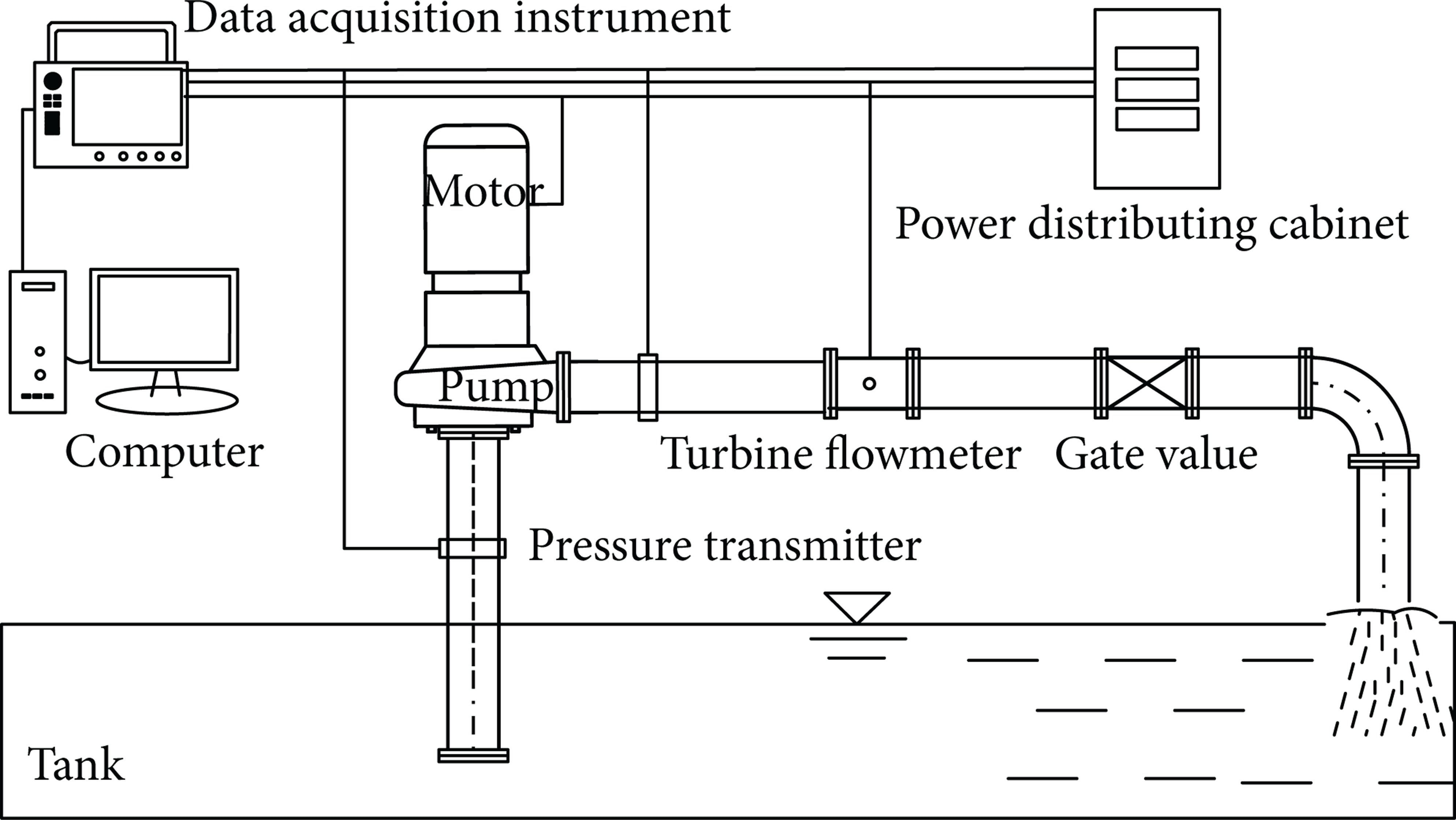
Test rig.

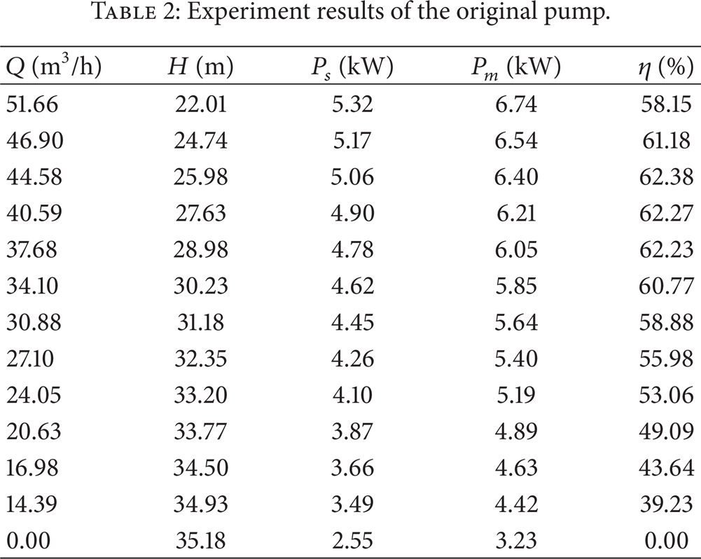
Test facilities and measurement methods abide by the relevant measurement requirements. The pump inlet and outlet pressure is measured by a pressure transmitter with 0.1% measurement error. The overall measurement uncertainty is calculated from the square root of the sum of the squares of the systematic and random uncertainties [28], and the calculated result of expanded uncertainty of efficiency is 0.5%. The performance of the original pump under multiflow rates was tested by experiments. Detailed experiments results were presented in Table 2.

Table 2:

Experiment results of the original pump.

Q (m³/h)	H (m)	P_s (kW)	P_m (kW)	η (%)

51.66	22.01	5.32	6.74	58.15
46.90	24.74	5.17	6.54	61.18
44.58	25.98	5.06	6.40	62.38
40.59	27.63	4.90	6.21	62.27
37.68	28.98	4.78	6.05	62.23
34.10	30.23	4.62	5.85	60.77
30.88	31.18	4.45	5.64	58.88
27.10	32.35	4.26	5.40	55.98
24.05	33.20	4.10	5.19	53.06
20.63	33.77	3.87	4.89	49.09
16.98	34.50	3.66	4.63	43.64
14.39	34.93	3.49	4.42	39.23
0.00	35.18	2.55	3.23	0.00

3. Numerical Simulation Methods

3.1. Meshes

The computational domain was modeled as the real machine, which include the impeller, volute, lateral cavity with seal leakage, balancing hole, inlet section, and outlet section. Unstructured grids were used in the volute, and all the other flow passages were meshed with structured girds. Considering that the wall functions were based on the logarithmic law, the maximum of the nondimensional wall distance was targeted to 30 < y⁺ < 80 in the mesh process. The total grid elements in the entire flow passages are approximately 1.6 million. Figure 3 gives a general view of the mesh in the impeller and the whole computation domain.

Figure 3:

Mesh sketch.

3.2. Methods and Boundary Conditions

The fully 3D incompressible Navier-Stokes equations are performed in ANSYS-CFX 13.0 code. The finite volume method has been used for the discretization of the governing equations, and the high resolution algorithm has been employed to solve the equations. Turbulence is simulated with the shear stress transport (SST) k-ω turbulence model. The space and pressure discretization scheme are set as second order accuracy.

In the steady state, the simulation is defined by means of the multireference frame technique, in which the impeller is situated in the rotating reference frame, and the volute is in the fixed reference frame, and they are related to each other through the “frozen rotor.” The grids of different domains are connected by using interfaces. At such interfaces, the flow fluxes are calculated based on the linear interpolation between the two sides, with fully implicit and fully conservative in flow fluxes. The boundary conditions are considered with the real operation conditions, as summarized in Table 3. Mass flow rate is specified in the pump inlet, and pressure outlet boundary is used at the pump exit. A smooth nonslip wall conditions have been imposed over all the physical surfaces, expect the interfaces between different parts. Maximum residuals are set to 10⁻⁵, and the mass flow value and static pressure value at the pump inlet and outlet are also monitored. When the overall imbalance of the four monitors is less than 0.1% or the maximum residuals are reached, the simulation was considered as steady and convergence.

Table 3:

Boundary conditions.

Position	Boundary condition

Inlet	Mass flow inlet
Outlet	Pressure outlet boundary
Walls	Nonslip wall
Impeller	Rotating reference frame
Volute	Stationary reference frame
Interface	General connection
Wall function	Automatic near-wall treatment

3.3. Performances Comparison

Through the numerical simulations under different flow rates, the detailed pump performance was obtained and compared with the experiments results, as shown in Figure 4. The comparison between test results and the numerical results has a good agreement, especially for the shaft power. In most cases, both the head and pump efficiency of simulation results are higher than experimental values. At design flow point, the simulation head is 29.21 m and pump efficiency is 64.11%; compared with the experimental head of 28.63 m and efficiency of 62.91%, the error is 2% and 1.9% in percent, respectively. For all the studied flow rates, the numerical results are consistent with the changing trends of the experimental data. It is clearly proven that the numerical methods used in this study could simulate the pump performance accurately.

Figure 4:

Experiment and simulation results comparisons of the original pump.

4. Orthogonal Experiments

4.1. Orthogonal Experiment Design

The effect of many different parameters on the overall performance characteristic in a condensed set of experiments can be examined by using the orthogonal experimental design. Once the parameters affecting a process that can be controlled have been determined, the levels at which these parameters should be varied must be determined. Determining what levels of a variable to test requires an in-depth understanding of the process, including the minimum, maximum, and interval for each level [13, 14].

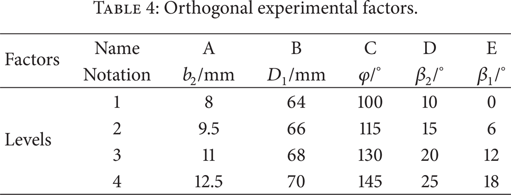
In this study, according to the manufacturers' requirements, the optimization just focuses on the impeller with an identical volute casing. Based on the impeller design experience, five important impeller geometrical factors were selected, namely, impeller outlet width b₂, impeller inlet diameter D₁, impeller blade wrapping angle φ, impeller blade outlet angle β₂, and impeller blade inlet angle β₁. Since the volute is keeping in the same geometry, the impeller parameters should stay in a reasonable range to match the volute. Therefore, according to the original pump characteristics and impeller design experience, four levels were chosen for each factor, as summarized in Table 4.

Table 4:

Orthogonal experimental factors.

Factors	Name	A	B	C	D	E
Factors	Notation	b₂/mm	D₁/mm	φ/°	β₂/°	β₁/°

Levels	1	8	64	100	10	0
	2	9.5	66	115	15	6
	3	11	68	130	20	12
	4	12.5	70	145	25	18

As long as the number of parameters and the number of levels are decided, the proper orthogonal table could be selected. Many predefined orthogonal tables have been given in the relative reference [13, 14]. These tables were created using an algorithm Taguchi developed and allows for each variable and setting to be tested equally. In the preset study, the orthogonal tables L₁₆ (4⁵) are used to arrange the experiments; five factors are evaluated each time and each factor takes four levels, and the detailed experimental programs are presented in Table 5.

Table 5:

Orthogonal experiment scheme.

No.	A	B	C	D	E

1	8	64	100	10	0
2	8	66	115	15	6
3	8	68	130	20	12
4	8	70	145	25	18
5	9.5	64	115	20	18
6	9.5	66	100	25	12
7	9.5	68	145	10	6
8	9.5	70	130	15	0
9	11	64	130	25	6
10	11	66	145	20	0
11	11	68	100	15	18
12	11	70	115	10	12
13	12.5	64	145	15	12
14	12.5	66	130	10	18
15	12.5	68	115	25	0
16	12.5	70	100	20	6

4.2. Orthogonal Experiment Results

According to the previous test scheme, the 16 impellers were designed and assembled with the same volute, respectively. Then, the 16 pumps were simulated in the ANSYS-CFX with the same computational methods of the original pump. Table 6 gives the predicted pump head and efficiency of the 16 programs at the design flow rate.

Table 6:

Numerical simulation results of the 16 programs under design point.

No.	H/m	η/%

1	27.89	64.57
2	28.19	65.93
3	28.04	66.40
4	27.24	63.23
5	30.14	66.38
6	30.00	67.13
7	30.07	66.94
8	30.05	66.81
9	32.05	66.94
10	31.36	66.93
11	31.30	66.38
12	30.67	66.82
13	31.87	67.42
14	30.74	67.49
15	32.98	65.84
16	32.54	64.42

Due to the orthogonal features, the importance order of each factor could be found through the analysis. These 16 test sets have tested all of the pairwise combinations of the independent variables. This demonstrates significant savings in testing effort over the all combinations approach. Variance analysis method (i.e., range analysis method) was used to clarify the significance levels of different influencing factors on the diameter and morphology of obtained fibers [13, 14], and those most significant factors could be disclosed basing the result of range analysis. The average values of each level for each factor were named as k_i, which is calculated as follows

k_{i} = \frac{1}{N_{i}} \sum_{j = 1}^{N_{i}} y_{i, j} .

(1)

The variances between each factor were defined as R to analyze the difference between the maximal and minimal value of the four levels for each factor:

R = \max (k_{1}, k_{2}, \dots, k_{i}) - \min (k_{1}, k_{2}, \dots, k_{i}),

(2)

where i is number of levels, j is number of factors,y_{i, j} is the performance value for factor j in level i, and N_i is the total number of levels, that is, N_i = 4 in this study.

The analysis results for pump efficiency were shown in Table 7 and Figure 5. As seen from Table 7, we find that the factor influence of the pump efficiency decreases in the order: A > B > C > E > D according to the R values. The impeller blade outlet width was found to be the most important determinant of efficiency. When the factor A employs the value of 11 mm, the pump has the highest efficiency. Factor D has the lower significant influence on the pump efficiency compared with the other factors. The reason maybe is that the volute in this paper is changeless. For all the five factors, their changing trends all have an obvious peak value; it means that each factors has a best value or levels for the better efficiency. Accordingly, the best program of optimized pump efficiency is A3, B2, C3, D2, and E3, namely, b₂ = 11 mm, D₁ = 66 mm, φ = 130°, β₂ = 15°, and β₁ = 12°.

Table 7:

Range analysis of pump efficiency.

	A	B	C	D	E

k ₁	65.032	66.328	65.625	66.455	66.037
k ₂	66.815	66.870	66.243	66.635	66.058
k ₃	66.767	66.390	66.910	66.032	66.942
k ₄	66.293	65.320	66.130	65.785	65.870

R	1.783	1.550	1.285	0.850	1.072

Figure 5:

Level influence of each factor for pump efficiency.

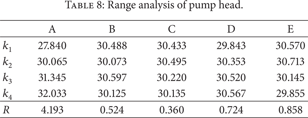
Table 8 is the range analysis of the head; the levels of influence are indicated in Figure 6. According to the R values, factor influence rank is A > E > D > B > C for the head. The primary factor that impacts the pump head is impeller outlet width. The best parameters combination for higher head is A4, B3, C2, D4, and E2, namely, b₂ = 12.5 mm, D₁ = 68 mm, φ = 115°, β₂ = 25°, and β₁ = 6°.

Table 8:

Range analysis of pump head.

	A	B	C	D	E

k ₁	27.840	30.488	30.433	29.843	30.570
k ₂	30.065	30.073	30.495	30.353	30.713
k ₃	31.345	30.597	30.220	30.520	30.145
k ₄	32.033	30.125	30.135	30.567	29.855

R	4.193	0.524	0.360	0.724	0.858

Figure 6:

Level influence of each factor for pump head.

4.3. Optimal Pump Performance

In this study, we focus on the pump efficiency improvement, so the optimal impeller design was adopted as A3, B2, C3, D2, and E3 (i.e., b₂ = 11 mm, D₁ = 66 mm, φ = 130°, β₂ = 15°, and β₁ = 12°) based on the results of the orthogonal experiment. Then, the final optimized impeller was designed and assembled with the same volute and simulated by the same numerical methods. Figure 7 compares the pump efficiency and head between the optimal pump and original pump, which are both predicted by the numerical methods.

Figure 7:

Predicted performance comparison between the original and optimal pumps.

At the design flow rate, the optimal pump has 67.55% efficiency and 30.93 m head. Compared with the original pump with 64.11% efficiency and 29.21 m, the increase is 5.4% and 5.9% in percent separately. In the pump operating flow range (0.8∼1.2 times design flow rate), the optimal pump has an obvious performance promotion. However, due to the influence of the volute, the optimal pump did not present a similar improvement in the smaller or larger flow area. It is indicated that the best way to optimize the pump drastically should be considering the design of the impeller and volute at the same time.

5. Conclusions

How to improve the impellers performance by changing their geometric characteristics is always challenging. In the present study, a centrifugal impeller was optimized by the orthogonal experiment method. The geometric parameters of the original pump were distributed clearly. Detailed numerical methods for pump performance prediction were presented, such as meshes, boundary conditions, and turbulence model. The original pump was manufactured and tested in a centrifugal pump test rig. Then, the numerical results of the original pump were compared with the experimental ones, and the comparisons between the two methods have a good agreement.

Five main impeller geometric characteristics were chosen as the research target to carry out the orthogonal experiment. The best programs for pump efficiency and head were obtained through the variance analysis method. The performance comparisons between the original pump and optimal pump show a remarkable improvement. The results also demonstrated that the impeller outlet width has the largest effect on both pump efficiency and head. But the optimal pump did not present an obvious improvement in the smaller or larger flow area. Therefore, the best way to optimize the pump performance should consider the impeller and volute together in the design process.

Footnotes

Notation

Acknowledgments

This work was supported by the National Natural Science Foundation of China Grant nos. 51279069 and 51109093 and National Studying Abroad Foundation of China. The authors would like to express their sincere gratitude to Professor Weigang Lu for his valuable guidance. Constructive suggestions from reviewers are also appreciated.

References

Gopalakrishnan

, “Pump research and development: past, present, and future—an American perspective,” Journal of Fluids Engineering, vol. 121, no. 2, pp. 237–247, 1999.

Hergt

P. H.

, “Pump research and development: past, present, and future,” Journal of Fluids Engineering, vol. 121, no. 2, pp. 248–253, 1999.

Zhou

Shi

W. D.

W. G.

, and Wu

, “Numerical investigations and performance experiments of a deep-well centrifugal pump with different diffusers,” Journal of Fluids Engineering, vol. 134, no. 7, Article ID 0711002, 8 pages, 2012.

Shojaeefard

M. H.

Tahani

Ehghaghi

M. B.

Fallahian

M. A.

, and Beglari

, “Numerical study of the effects of some geometric characteristics of a centrifugal pump impeller that pumps a viscous fluid,” Computers and Fluids, vol. 60, pp. 61–70, 2012.

Anagnostopoulos

J. S.

, “A fast numerical method for flow analysis and blade design in centrifugal pump impellers,” Computers and Fluids, vol. 38, no. 2, pp. 284–289, 2009.

Yuhki

Hatoh

Nogawa

Miura

Shimazaki

, and Takatani

, “Detection of suction and regurgitation of the implantable centrifugal pump based on the motor current waveform analysis and its application to optimization of pump flow,” Artificial Organs, vol. 23, no. 6, pp. 532–537, 1999.

Visser

F. C.

Dijkers

R. J. H.

, and Woerd

J. G. H.

, “Numerical flow-field analysis and design optimization of a high-energy first-stage centrifugal pump impeller,” Computing and Visualization in Science, vol. 3, no. 1–2, pp. 103–1082000.

Pierret

and Van Den Braembussche

R. A.

, “Turbomachinery blade design using a Navier-Stock solver and artificial neural network,” Journal of Turbomachinery, vol. 121, no. 2, pp. 326–332, 1999.

Amaral

Verstraete

Van den Braembussche

, and Arts

, “Design and optimization of the internal cooling channels of a high pressure turbine blade-Part I: methodology,” Journal of Turbomachinery, vol. 132, no. 2, Article ID 021013, 7 pages, 2010.

10.

and Shan

, “Three-dimensional aerodynamic optimization for axial-flow compressors based on the inverse design and the aerodynamic parameters,” Journal of Turbomachinery, vol. 134, no. 3, Article ID 031004, 2011.

11.

Ahn

C.-S.

and Kim

K.-Y.

, “Aerodynamic design optimization of a compressor rotor with Navier-Stokes analysis,” Proceedings of the Institution of Mechanical Engineers A, vol. 217, no. 2, pp. 179–184, 2003.

12.

Song

, and Feng

, “2D viscous aerodynamic shape design optimization for turbine blades based on adjoint method,” Journal of Turbomachinery, vol. 133, no. 3, Article ID 031014, 2011.

13.

Roy

R. K.

, Design of Experiments Using Taguchi Approach: 16 Steps to Product and Process Improvement, John Wiley & Sons, New York, NY, USA, 2001.

14.

Ross

P. J.

, Taguchi Techniques for Quality Engineering, Mc-Graw Hill, New York, NY, USA, 1988.

15.

Rao

R. S.

Kumar

C. G.

Prakasham

R. S.

, and Hobbs

P. J.

, “The Taguchi methodology as a statistical tool for biotechnological applications: a critical appraisal,” Biotechnology Journal, vol. 3, no. 4, pp. 510–523, 2008.

16.

Byrne

D. M.

and Taguchi

, “The Taguchi approach to parameter design,” Quality Progress, vol. 20, no. 12, pp. 19–26, 1987.

17.

Cui

Zhou

, and Weng

, “Investigation on process parameters of electrospinning system through orthogonal experimental design,” Journal of Applied Polymer Science, vol. 103, no. 5, pp. 3105–3112, 2007.

18.

Chen

Hong

, and Harris

C. J.

, “Sparse kernel regression modeling using combined locally regularized orthogonal least squares and D-optimality experimental design,” IEEE Transactions on Automatic Control, vol. 48, no. 6, pp. 1029–1036, 2003.

19.

Zhou

Zhang

Xie

Chen

, and Duan

, “Infrared-assisted extraction of adenosine from radix isatidis using orthogonal experimental design and LC,” Chromatographia, vol. 72, no. 7–8, pp. 719–724, 2010.

20.

Wang

and Tsukamoto

, “Experimental and numerical study of unsteady flow in a diffuser pump at off-design conditions,” Journal of Fluids Engineering, vol. 125, no. 5, pp. 767–778, 2003.

21.

Engin

and Kurt

, “Prediction of centrifugal slurry pump head reduction: an artificial neural networks approach,” Journal of Fluids Engineering, vol. 125, no. 1, pp. 199–202, 2003.

22.

Pedersen

Larsen

P. S.

, and Jacobsen

C. B.

, “Flow in a centrifugal pump impeller at design and off-design conditions—part I: particle image velocimetry (PIV) and laser Doppler velocimetry (LDV) measurements,” Journal of Fluids Engineering, vol. 125, no. 1, pp. 61–72, 2003.

23.

Byskov

R. K.

Jacobsen

G. B.

, and Pedersen

, “Flow in a centrifugal pump impeller at design and off-design conditions—part II: large eddy simulations,” Journal of Fluids Engineering, vol. 125, no. 1, pp. 73–83, 2003.

24.

Choi

Y.-D.

Kurokawa

, and Malsui

, “Performance and internal flow characteristics of a very low specific speed centrifugal pump,” Journal of Fluids Engineering, vol. 128, no. 2, pp. 341–349, 2006.

25.

Majidi

, “Numerical study of unsteady flow in a centrifugal pump,” Journal of Turbomachinery, vol. 127, no. 2, pp. 363–371, 2005.

26.

Shi

Zhou

Pei

, and Lang

, “Numerical prediction and performance experiment in a deep-well centrifugal pump with different impeller outlet width,” Chinese Journal of Mechanical Engineering, vol. 26, no. 1, pp. 46–52, 2013.

27.

ISO, “9906 Rotodynamic Pumps-Hydraulic performance acceptance tests-Grades 1 and 2,” International Standardization Organization, Geneva, Switzerlands, 1999.

28.

Feng

H. D.

R. P.

, “Uncertainty analysis using the thermodynamic method of pump efficiency testing,” Proceedings of the Institution of Mechanical Engineers C, vol. 218, pp. 543–555, 2004.

Performance Optimization in a Centrifugal Pump Impeller by Orthogonal Experiment and Numerical Simulation

Abstract

1. Introduction

2. Geometry and Experiment

2.1. Geometric Model

2.2. Performance Experiment

3. Numerical Simulation Methods

3.1. Meshes

3.2. Methods and Boundary Conditions

3.3. Performances Comparison

4. Orthogonal Experiments

4.1. Orthogonal Experiment Design

4.2. Orthogonal Experiment Results

4.3. Optimal Pump Performance

5. Conclusions

Footnotes

Notation

Acknowledgments

References