Sage Journals: Discover world-class research

Abstract

The liquid turbulence modulation by small bubbles was investigated detailedly in a vertical upward channel flow with a finite number of small bubbles with the developed Eulerian-Lagrangian method. Small bubbles are treated as pointwise spheres subject to gravity, drag, added mass, pressure gradient, lift, and wall lift forces. The momentum transfer between phases was realized through interphase forces. The present investigation shows that the liquid turbulence is intensified near the wall and is slightly weakened in the channel central region due to the bubble addition. The turbulence modulation mechanisms by bubbles were also analyzed in the paper.

1. Introduction

Bubbly flows exist extensively in industrial processes such as two-phase heat exchangers, bubble column reactors, smelting of metals, aeration and stirring of reactors, air-conditioning engineering, wastewater treatment, fermentation reactions, mineral floatation, cavitating flows, and transportation lines, [1 –3]. The above applications have stimulated many researches on bubbly flows and have demanded a deep understanding of bubbly hydrodynamics. Therefore, the bubbly flow has received much attention in the academic world over the past 30 years. Of numerous study contents on the bubbly flow, it is very important to accurately and quantitatively understand the turbulence modulation by bubbles, because it controls directly heat transfer and mixing efficiency of bubbly flows and the drag reduction rate by bubbles.

Currently, some researchers had performed definite studies on the turbulence modulation by bubbles and had obtained some important conclusions. Serizawa and Kataoka summarized three kinds of turbulence suppression mechanisms [4]. Kato et al. deduced that the bubble influencing the liquid turbulence is just like the influence of the solid particle on the gas turbulence: large bubbles enhance the liquid-phase turbulence, whereas small bubbles reduce the liquid turbulence [5]. This view is also accepted by Kim et al. [6], and they pointed out that when there is no change in volume of the dispersed phase, the turbulence production and dissipation can be understood by similar mechanisms. So et al. [7] and Molin et al. [8] considered that the lift force direction and magnitude are sensitive to the bubble size, so it is possible that the reason for the suppressed velocity fluctuations is the modification of the global flow structure caused by the bubble accumulation near the wall. Kawamura and Kodama [9] pointed out that the bubble can influence velocity fluctuations in two ways: one is the so-called “pseudo-turbulence” and the other is the liquid-phase turbulence modulated by bubbles. Mazzitelli et al. considered that microbubbles accumulating in down-flow regions locally transfer momentum upwards, and, therefore, the microbubble addition reduces the vertical velocity fluctuation intensity and the turbulent kinetic energy [10]. Ferrante and Elghobashi argued that microbubbles in a spatially developing turbulent boundary layer push the developing streamwise vortices away from the wall, leading to less dissipation in the boundary layer [11]. Van den Berg et al. pointed out that the microbubbles modulation on the turbulence is a boundary layer effect [12]. Lu and Tryggvason believed that bubble deformation has a great influence on the liquid turbulence [13]. Yeo et al. considered that the turbulence modulation only slightly depends on the dispersion characteristics but is closely related to the stresslet component of flow disturbances [14].

From the above review, one can see that many investigations on the turbulence modulation by bubbles have been performed, but the turbulence modulation mechanism is still not clear. That is just our study motivation. In order to understand the turbulence modulation mechanism by bubbles, an Eulerian-Lagrangian method was developed and applied to simulate a bubbly flow laden with finite number bubbles. The liquid-phase velocity field was solved with direct numerical simulations, and the bubble trajectories were tracked by Newtonian motion equations. The interphase momentum coupling was realized through considering the interphase force as a momentum source term of the liquid phase. For the present investigation, hydrodynamic direct interactions between bubbles were negligible due to the low global void fraction (α₀ < 10⁻³) according to Elghobashi [15], and Bunner and Tryggvason [2] also verified that the spherical bubbles never touch in the dilute bubbly flow. The bubble deformation and breakup were also neglected due to the too small diameter (Weber number, We ≪1) [16].

2. Computational Condition and Method

A vertical channel flow laden with small bubbles (see Figure 1) is simulated, and gravity is s directed along the negative x direction. The size of the computational domain is x × y × z = 10 h × 2 h × 5 h, where h is the channel half width. Note that the x, y, and z axes denote the streamwise, wall-normal, and spanwise directions, respectively. The flow field and the bubble motion are periodic both in the stream-wise and in the spanwise directions, while no-slip conditions are imposed on the channel wall for liquid, and the wall elastic collision reflection condition is used in the wall-normal direction for bubbles. The flow is driven by an imposed pressure gradient, with bubbles seeded at a void fraction low enough to ensure the dilute system condition and negligible bubble-bubble interactions. For the bubbly simulation, when a statistically steady state of the liquid turbulence is reached, the bubbles are injected into the flow. The liquid phase is considered to be incompressible, isothermal, and with constant properties, and its thermophysical property data are used as that of water at room temperature, ρ_f = 1000 kg/m³. The bubbles are regarded as spherical in shape, and their density is ρ_b = 1.3 kg/m³. The bubble diameter is d_b = 0.011h, and the global void fraction is α₀ = 1.34 × 10⁻⁴.

Figure 1:

The simulation domain and coordinate system.

2.1. Equations for the Liquid Phase

For the present investigation, the governing equations for the liquid phase are continuity equation and a modified Navier-Stokes equation in which the feedback force on the liquid is included as an effective body force. Governing equations of the liquid phase in the dimensionless form are presented as follows. The normalized process of the related parameters can be referred to the literature [17]:

\frac{\partial u_{f_{i}}^{+}}{\partial x_{i}^{*}} = 0,

(1)

\frac{\partial u_{f_{i}}^{+}}{\partial t^{*}} + u_{f_{j}}^{+} \frac{\partial u_{f_{i}}^{+}}{\partial x_{j}^{*}} = - \frac{\partial {p^{+}}^{*}}{\partial x_{i}^{*}} + δ_{1 i} + \frac{1}{R e_{τ}} \nabla^{2} u_{f_{i}}^{+} - \overset{—}{f_{i}^{*}},

(2)

where u_i is the ith component of the liquid velocity vector, p is the fluctuating kinematic pressure, δ_1i is the mean pressure gradient that drives the liquid flow, and Re_τ = u_τh/υ_f is the shear Reynolds number based on the shear velocity (u_τ = (δ_1ih/ρ_f)^1/2). Note that bubbles cause pressure drop changes so the shear velocity is not defined using the shear stress at the wall (τ_w) as usually done in the single-phase system. The last term on the right-hand side of (2), $\overset{—}{f_{i}^{*}}$ , represents the interphase momentum coupling, given by the force per unit mass exerted by the bubbles on the liquid, and is modeled using the famous particle-source-in-cell method proposed by Crowe et al. [18].

Equations (1) and (2) were solved directly using a finite difference scheme. A second-order central difference scheme was applied to discrete the spatial term. For the time integration, the Adams-Bashforth scheme is used for all the terms except that the implicit method is used for the pressure term. The velocity-pressure coupling is made with the MAC method. A staggered grid system is used to prevent a checkboard pressure field, which leads to the fact that velocity components are located at cell faces and other variables are located at cell centers. The uniform meshes are used in the x and z directions, whereas the nonuniform meshes are adopted in the y direction. The grid system of 64³ meshes is adopted. The grid spacings in the streamwise and spanwise directions are Δx⁺ = 2.34 and Δz⁺ = 11.7, respectively. Δy⁺ varies from 0.45 next to the wall to about 9 near the center of the flow. The incompressibility condition results in a nonseparable elliptic equation for the pressure term, for which a multiple grid solver is developed. The basic numerical method is described in detail in [19].

2.2. Equations for the Bubble Phase

The single bubble motion is computed by solving Newton motion equation in the Lagrangian frame. It can be given as follows:

\frac{ρ_{b}}{ρ_{f}} \frac{d u_{b_{i}}^{+}}{d t^{*}} = \frac{D u_{f_{i}}^{+}}{D t^{*}} + \frac{3}{4} \frac{C_{D}}{d_{b}^{*}} | u_{f_{i}}^{+} - u_{b_{i}}^{+} | (u_{f_{i}}^{+} - u_{b_{i}}^{+}) + C_{v} (\frac{D u_{f_{i}}^{+}}{D t} - \frac{d u_{b_{i}}^{+}}{d t^{*}}) + C_{LF} ∊_{i j k} ∊_{k l m} (u_{f_{i}}^{+} - u_{b_{i}}^{+}) \frac{\partial u_{f_{i}}^{+}}{\partial x_{m}^{*}} + δ_{2 i} {| u_{f_{i}}^{+} - u_{b_{i}}^{+} |}^{2} \max (0, \frac{- 0.0064}{d_{b}^{*}} + \frac{0.016}{y_{b}^{*}}) + (1 - \frac{ρ_{b_{i}}}{ρ_{f}}) \frac{1}{F r^{2}},

(3)

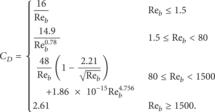
where u_i is the ith component of the velocity vector, ρ is the density, y_b is the distance between the bubble and the wall, ∊ is sign of permutation, t is the time variable, and x is the coordinate variable. Fr is the Froude number, Fr = u_τ/(gh)^1/2. Subscripts b and f denote the bubble and liquid phase, respectively. In (3), the right-hand terms are the pressure gradient force, the drag force, the added mass force, the shear lift force, the wall lift force, and the buoyant force, respectively. The wall lift force is calculated according to Krepper et al. [20]. For the spherical bubble, the added mass force coefficient is C_v = 0.5. The drag coefficient is calculated by the empirical correlation developed by Laín et al. [21], and the lift coefficient is computed with the expression developed by Legendre and Magnaudet [22]. The drag coefficient is expressed as follows:

C_{D} = {\begin{cases} \frac{16}{R e_{b}} & R e_{b} \leq 1.5 \\ \frac{14.9}{R {e_{b}^{0.78}}_{}} & 1.5 \leq R e_{b} < 80 \\ \begin{matrix} \frac{48}{R e_{b}} (1 - \frac{2.21}{\sqrt{R e_{b}}}) \\ + 1.86 \times 1 0^{- 15} R e_{b}^{4.756} \end{matrix} & 80 \leq R e_{b} < 1500 \\ 2.61 & R e_{b} \geq 1500 . \end{cases}

(4)

The lift coefficient, C_LF, is written as

C_{LF} = κ \sqrt{{C_{L}^{low Re} (R e_{b}, S r_{b})}^{2} + {C_{L}^{high Re} (R e_{b})}^{2}},

(5)

where

\begin{matrix} C_{L}^{low Re} (R e_{b}, S r_{b}) = \frac{6}{π^{2}} {(R e_{b} \cdot S r_{b})}^{- 0.5} \times [\frac{2.255}{{(1 + 0.2 ζ^{- 2})}^{1.5}}], \\ C_{L}^{high Re} (R e_{b}) = \frac{1}{2} (\frac{1 + 16 / R e_{b}}{1 + 29 / R e_{b}}) \begin{matrix} , \end{matrix} \\ κ = 2 - \exp (2.92 {d_{b}^{*}}^{2.21}) \end{matrix}

(6)

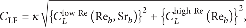
where Sr_b and Re_b are the nondimensional shear rate and the bubble Reynolds number defined as $S r_{b} = | ω_{b} | d_{b} / 2 | u_{f} - u_{b} |$ and $R e_{b} = | u_{f} - u_{b} | d_{b} / v_{f}$ , respectively. Here, d_b is the bubble diameter, ω_b is the velocity gradient around the bubble, and $ζ = \sqrt{S r_{b} / R e_{b}}$ . The time derivative Du/Dt = ∂ u/∂ t + u · ∇ u is the total acceleration of the liquid at the bubble location, whereas du/dt = ∂ u/∂ t + u · ∇ u is calculated along bubble trajectories.

To analyze the effect that bubbles exert collectively on the liquid turbulence, the flow should be laden with O(10⁴) bubbles at least [8]. Because there is a limit to the present computational capability, it is not feasible to track such many bubbles using fully resolved simulations. An alternative Eulerian-Lagrangian approach was developed so as to track large swarms of bubbles at reduced computational costs by the following method: (i) regarding bubbles as points, (ii) neglecting interactions among bubbles, and (iii) using effective force models for the interphase force.

The trajectory of each bubble is computed simultaneously in time with the liquid-phase equations. The motion equation of each bubble, for the time advancement, is solved using the second-order Crank-Nicholson scheme. To calculate interphase forces related to the relative velocity between the bubble and local liquid, a three-dimensional 8-node combined with a two-dimensional 4-node Lagrangian interpolation polynomials are used to compute velocities of liquid at the same positions of bubbles (near the wall, the interpolation scheme switches to one-sided).

3. Results and Discussion

3.1. Bubble Distribution

It was reported that the lateral distribution of bubbles plays an important role in understanding the liquid turbulence modulation by bubbles, and thus the bubble distribution was investigated firstly. Figure 2 shows the lateral distribution of bubbles along the wall-normal direction. Figure 2(a) displays the instantaneous distribution of bubbles when the bubble motions reach a statistically steady state. It can be seen from Figure 2(a) that a large swarm of bubbles accumulate near the walls, whereas a minority of bubbles scatter evenly in a wide central region of the channel. Figure 2(b) shows the statistical distribution of bubbles for statistically steady states. It shows that the present distribution pattern of bubbles is somewhat similar to the wall-peaked profile; that is, a sharp peak with relatively high void fraction appears near the wall and a plateau with very low void fraction around the wide central region of the channel. Many investigations show that a great peak appearance near the wall is related to the shear lift force [23]. Bubbles move firstly toward the wall from the central under the aid of the turbulence and then slowly approach to the wall under the assistance of the lift force. Note that bubbles only stay at the balance region between the lift force and the drag force, and they cannot come into contact with the wall due to the limit of the wall lift force too.

Figure 2:

The lateral distribution of bubbles in the channel.

3.2. Turbulence Modulation by Bubbles

In order to understand the liquid turbulence modulation by bubbles, the bubbles influence on the turbulence statistics of the liquid phase was analyzed in detail. Figure 3 shows average velocity profiles of the liquid and bubble phases. One can see from Figure 3 that the bubble moves faster than the liquid due to the buoyancy pulling, and the liquid without bubbles flows slightly slower than the liquid laden with bubbles. Our previous studies showed that the increase of the liquid-phase velocity has a direct relation to the bubble drag in the gravitational field; namely, due to the buoyancy force, the bubbles move faster that the liquid, and then the bubbles drag the liquid acceleration, which leads to the increase of the liquid-phase velocity, and it seems to have nothing to do with the liquid turbulence suppressions by bubbles for the dilute bubbly flow [24]. It was also checked that the reduction in weight of the mixture influences the liquid velocity, and it was discovered that the liquid velocity increasing rate is far higher than the reduction rate in weight of the mixture. And thus, it can be concluded that the liquid velocity increase seems to have little to do with the reduction in weight of the mixture due to the bubble addition. It needs to be further investigated whether the liquid turbulence suppressions can cause the increase of the liquid velocity for the dense bubbly flow. However, it is a pity that the presently developed method cannot deal with the dense bubbly flow laden with a huge mount of bubbles due to the huge computation cost.

Figure 3:

Average velocity profiles.

Figure 4 shows turbulence intensity profiles of the liquid with and without bubbles. It shows that the bubble injection, to a different degree, reduces the liquid-phase turbulence intensity components in the lateral direction compared with ones of the single-phase flow in the whole channel, whereas it shows different influences on the streamwise component of the turbulence intensity; that is, the streamwise component of the turbulence intensity is increased near the wall, and it is reduced in the channel central region. To examine the general influence of bubbles on the liquid turbulence, the turbulence modulation was defined as follows in [25]:

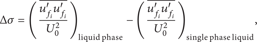
Δ σ = {(\frac{\overset{—}{{u_{f_{i}}^{'}}_{}^{} u_{f_{i}}^{'}}}{U_{0}^{2}})}_{liquid phase} - {(\frac{\overset{—}{u_{f_{i}}^{'} u_{f_{i}}^{'}}}{U_{0}^{2}})}_{single phase liquid},

(7)

where U₀ is the mean velocity of the pure liquid at the channel centre, $\overset{—}{u_{f_{i}}^{'} u_{f_{i}}^{'}}$ is the liquid velocity variance, $\overset{—}{u_{f_{i}}^{'} u_{f_{i}}^{'}} = \overset{—}{u^{'} u^{'}} + \overset{—}{v^{'} v^{'}} + \overset{—}{w^{'} w^{'}}$ . Figure 5 shows the turbulence modulation profile. It can be seen from Figure 5 that the liquid turbulence is enhanced in the region near the wall, and it is suppressed in the channel central region. The enhancement of the liquid turbulence near the wall probably relates to the fact that a large number of bubbles swarm near the wall, which causes their wakes to come into being interactions. Especially in the streamwise direction, the wake interactions of bubbles are relatively intenser than those in the lateral direction due to a high velocity. That corresponds to the fact that the streamwise component of the turbulence intensities is strengthened near the wall due to the bubble injection.

Figure 4:

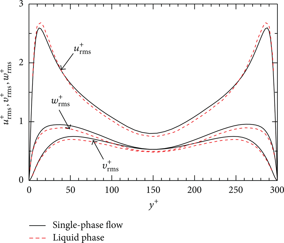
Turbulence intensity profiles.

Figure 5:

Turbulence modulation profile.

In the channel central region, the liquid turbulence suppression may be explained by the following two mechanisms. One is that the bubbles move faster than the liquid due to the buoyancy effect; that is, the bubbles flow faster than the turbulence vortexes, which leads to the fact that the bubbles can quickly pass through a variety of the liquid turbulence vortexes, and thus they can cause a variety of vortexes to attenuate and even to vanish, as shown in Figure 6(a). The other is that a violent accumulation of bubbles near the wall can prevent the spanwise vortex from developing and propagating, which further leads to the decrease of the streamwise vortex since the streamwise vortex evolves from the spanwise vortex, as shown in Figure 6(b).

Figure 6:

Models of bubbles influencing liquid turbulence vortex.

The liquid turbulent intensity and vortex changes are bound to change Reynolds shear stress. Figure 7 displays the influence of the bubbles on the Reynolds shear stress. It can be seen that the bubble addition reduces the liquid-phase Reynolds shear stress compared with the single liquid-phase one. Due to its complexity of the Reynolds shear stress, it is relatively difficult to ascertain its changing reasons. To understand the detailed contribution to the total turbulence production from different events in a turbulent flow, and to provide information on the influence of the bubbles on each contribution, the quadrant analysis of the fluctuating velocity field is carried out. Figure 8 exhibits the fractional contribution of the Reynolds shear stress from different quadrant motions. One can see that the bubble addition has greater influence on the second (𝒬₂) and fourth quadrant (𝒬₄) motions than on the first (𝒬₁) and third quadrant (𝒬₃) ones. That means that the bubbles significantly suppress the ejection and sweep motions occurring near the wall, which results in a reduction of the liquid-phase Reynolds shear stress.

Figure 7:

Reynolds shear stress profile.

Figure 8:

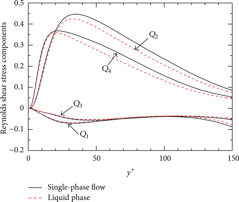
Quadrant analysis of Reynolds shear stress.

Figure 9 shows the instantaneous secondary velocity vectors distribution of the liquid at a z-y plane. It shows that the busting events of the liquid turbulence are weakened by the bubble injection near the wall, and the circulation spatial size is larger for the flow laden with bubbles than one for the single-phase flow. That corresponds to the fact that the liquid fluctuation components are reduced due to the bubble injection, as shown in Figure 4.

Figure 9:

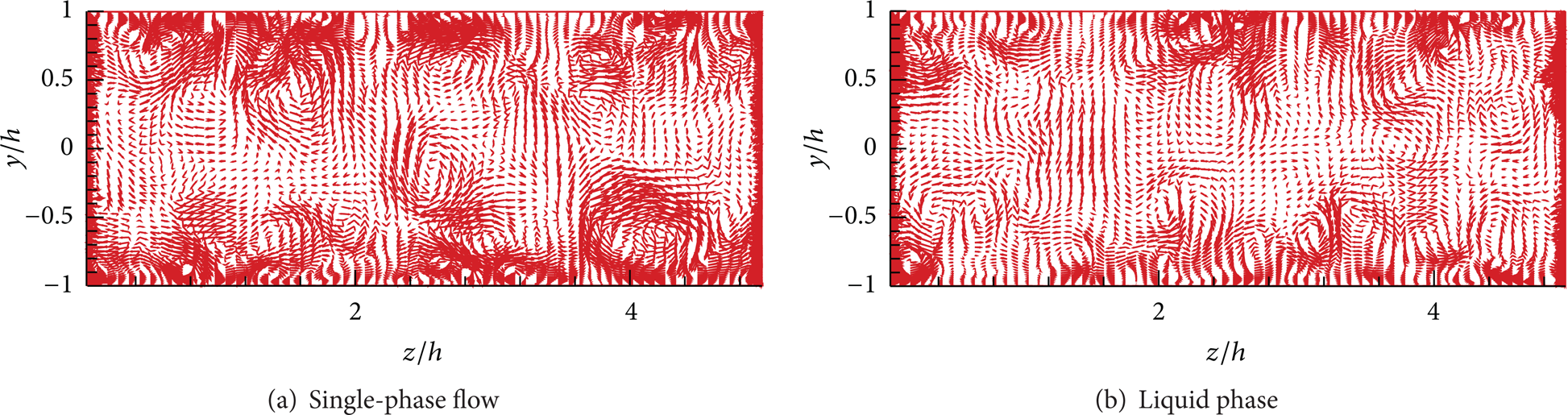
Instantaneous velocity distribution.

4. Conclusions

The turbulence modulation by small bubbles was studied with the developed quasidirect numerical simulation method, and several important conclusions can be summarized as follows.

Bubbles move violently toward the wall under the aid of the shear lift force and the turbulence, which leads to the present distribution pattern similar to the typical wall-peaked profile.

The bubble injection leads to the liquid velocity increase by the bubble pulling, slightly intensifies the liquid turbulence due to mutual influence of bubble wakes near the wall, and somewhat weakens the liquid turbulence in the channel central region. In the channel central region, the liquid turbulence suppression may be related to the vortex decay by a single bubble and the spanwise vortex prevention by a bubble swarm.

The bubble addition reduces the liquid-phase Reynolds stress due to the turbulence ejection and sweep motions suppressed by the bubbles.

Footnotes

Acknowledgments

The authors gratefully acknowledge the financial support from the NSFC Fund (nos. 51225601 and 51076124) and the Specialized Research Fund for the Doctoral Program of Higher Education of China (no. 20090201110002).

References

Magnaudet

and Eames

, “The motion of high-reynolds-number bubbles in inhomogeneous flows,” Annual Review of Fluid Mechanics, vol. 32, pp. 659–708, 2000.

Bunner

and Tryggvason

, “Effect of bubble deformation on the properties of bubbly flows,” Journal of Fluid Mechanics, no. 495, pp. 77–118, 2003.

Guet

and Ooms

, “Fluid mechanical aspects of the gas-lift technique,” Annual Review of Fluid Mechanics, vol. 38, pp. 225–249, 2006.

Serizawa

and Kataoka

, “Turbulence suppression in bubbly two-phase flow,” Nuclear Engineering and Design, vol. 122, no. 1–3, pp. 1–16, 1990.

Kato

Iwashina

Miyanaga

, and Yamaguchi

, “Effect of microbubbles on the structure of turbulence in a turbulent boundary layer,” Journal of Marine Science and Technology, vol. 4, no. 4, pp. 155–162, 2000.

Kim

S. Y.

Lee

K. B.

, and Lee

C. G.

, “Theoretical approach on the turbulence intensity of the carrier fluid in dilute two-phase flows,” International Communications in Heat and Mass Transfer, vol. 32, no. 3–4, pp. 435–444, 2005.

Morikita

Takagi

, and Matsumoto

, “Laser doppler velocimetry measurement of turbulent bubbly channel flow,” Experiments in Fluids, vol. 33, no. 1, pp. 135–142, 2002.

Molin

Marchioli

, and soldati

, “Turbulence modulation and microbubble dynamics in vertical channel flow,” International Journal of Multiphase Flow, vol. 42, no. 6, pp. 80–95, 2012.

Kawamura

and Kodama

, “Numerical simulation method to resolve interactions between bubbles and turbulence,” International Journal of Heat and Fluid Flow, vol. 23, no. 5, pp. 627–638, 2002.

10.

Mazzitelli

I. M.

Lohse

, and Toschi

, “The effect of microbubbles on developed turbulence,” Physics of Fluids, vol. 15, no. 1, pp. L5–L8, 2003.

11.

Ferrante

and Elghobashi

, “On the physical mechanisms of drag reduction in a spatially developing turbulent boundary layer laden with microbubbles,” Journal of Fluid Mechanics, no. 503, pp. 345–355, 2004.

12.

van den Berg

T. H.

van Gils

D. P. M.

Lathrop

D. P.

, and Lohse

, “Bubbly turbulent drag reduction is a boundary layer effect,” Physical Review Letters, vol. 98, no. 8, Article ID 084501, 2007.

13.

J. C.

and Tryggvason

, “Effect of bubble deformability in turbulent bubbly upflow in a vertical channel,” Physics of Fluids, vol. 20, no. 4, Article ID 040701, 2008.

14.

Yeo

Dong

Climent

, and Maxey

M. R.

, “Modulation of homogeneous turbulence seeded with finite size bubbles or particles,” International Journal of Multiphase Flow, vol. 36, no. 3, pp. 221–233, 2010.

15.

Elghobashi

, “On predicting particle-laden turbulent flows,” Applied Scientific Research, vol. 52, no. 4, pp. 309–329, 1994.

16.

Detsch

, “Small air bubbles in reagent grade water and seawater: I. Rise velocities of 20 to 1000 μm diameter bubbles,” Journal of Geophysical Research, vol. 96, no. 5, pp. 8901–8906, 1991.

17.

Pang

M. J.

Wei

J. J.

, and Yu

, “Numerical study of bubbly upflows in a vertical channel using the Euler-Lagrange two-way model,” Chemical Engineering Science, vol. 65, no. 23, pp. 6215–6228, 2010.

18.

Crowe

C. T.

Stock

D. E.

, and Sharma

M. P.

, “The Particle-Source-In Cell (PSI-CELL) model for gas-droplet flows,” Journal of Fluids Engineering, vol. 99, no. 2, pp. 325–332, 1977.

19.

and Kawaguchi

, “Direct numerical simulation of viscoelastic drag-reducing flow: a faithful finite difference method,” Journal of Non-Newtonian Fluid Mechanics, vol. 116, no. 2–3, pp. 431–466, 2004.

20.

Krepper

Lucas

, and Prasser

H. M.

, “On the modelling of bubbly flow in vertical pipes,” Nuclear Engineering and Design, vol. 235, no. 5, pp. 597–611, 2005.

21.

Laín

Bröder

, and Sommerfeld

, “Modeling hydrodynamics and turbulence in a bubble column using the Euler-Lagrange procedure,” International Journal of Multiphase Flow, vol. 28, no. 6, pp. 1381–1407, 2002.

22.

Legendre

and Magnaudet

, “The lift force on a spherical bubble in a viscous linear shear flow,” Journal of Fluid Mechanics, vol. 368, pp. 81–126, 1998.

23.

Antal

S. P.

Lahey

J. R. T.

, and Flaherty

J. E.

, “Analysis of phase distribution in fully developed laminar bubbly two-phase flow,” International Journal of Multiphase Flow, vol. 17, no. 5, pp. 635–652, 1991.

24.