Sage Journals: Discover world-class research

Abstract

This paper presents an integer linear programming model devoted to optimize the energy consumption efficiency in heterogeneous wireless sensor networks. This model is based upon a schedule of sensor allocation plans in multiple time intervals subject to coverage and connectivity constraints. By turning off specifics sets of redundant sensors in each time interval, it is possible to reduce the total energy consumption in the network and, at the same time, avoid partitioning the whole network by losing some strategic sensors too prematurely. Since the network is heterogeneous, sensors can sense different phenomena from different demand points, with different sample rates. By resorting to this model, it is possible to provide extra lifetime to heterogeneous wireless sensor networks, reducing their setup and maintenance costs. This is an important issue to be considered when deploying sensor devices in hostile and inaccessible environments.

1. Introduction

A wireless Sensor Network (WSN) typically consists of a large number of small, low-power, and limited-bandwidth computational devices named sensor nodes, as shown in Figure 1. Four modules constitute a sensor node: processor, battery, transmission, and sensor module. In addition to the construction of processing packets, a dynamic algorithm for routing in sensor nodes is performed to find and configure the best possible network topology at runtime in order to reduce the loss of energy and retransmission.

Figure 1

Sensor node.

These nodes can frequently interact with each other, in a wireless manner, in order to relay the sensed data towards one or more processing machines (also known as sinks) residing outside the network. They also have been primarily used in the monitoring of several physical phenomena, such as temperature, barometric pressure, humidity, ambient light, sound volume, solar radiation, and precipitation, and therefore have been deployed in different areas of application/research, like agriculture, climate study, biology, and security. Figure 2 outlines a wireless sensor network.

Figure 2

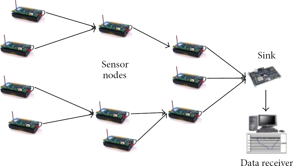
Wireless sensor networks.

The simple deployment of the approach is proposed by [1], while sensing different phenomena through the same WSN can lead to inefficiency in terms of energy expenditure. With this perspective in mind, in this work, we provide an extension to the model devised by [2–4], namely, to consider different coverage radius and sampling rates for different phenomena. We argue that the incorporation of such aspects into the model can have a significant impact on the network lifetime mainly when the spatiotemporal properties of the phenomena under observation vary a lot.

The introduction of this new dimension into the model brings about novel issues to be dealt with. The critical issue relates to the concurrent routing of data related to different phenomena, as these data should be relayed to different sinks. The rest of the paper is organized as follows. Section 2 presents the Wireless Sensor Network (WSN), how do they work, the components of a sensor, the problems that can occur in a WSN, and complementary knowledge to optimize the network. On the other hand, Section 3 presents the novel integer linear programming model for the minimization of energy expenditure in WSNs regarding the heterogeneity aspects of the sensed phenomena mentioned above. Moreover, Section 4 presents computational results achieved by simulation while providing a qualitative discussion of such results. Finally, Section 5 concludes the paper and comments on future work.

2. The Wireless Sensor Network

A Wireless Sensor network typically consists of a large number of small, low-power, and limited-bandwidth computational devices named sensor nodes. These nodes can frequently interact with each other, in a wireless manner, in order to relay the sensed data towards one or more processing machines (a.k.a. sinks) residing outside the network [5]. For such a purpose, special devices, called gateways, are also employed in order to interface the WSN with a wired transport network. To avoid bottleneck and reliability problems, it is pertinent to make one or more of these gateways available in the same network setting. This is a strategy that can also reduce the length of the traffic routes across the network and consequently lower the overall energy consumption. A typical sensor node is composed of four modules, namely, the processing module, the battery, the transceiver module, and the sensor module [6]. Besides the packet building processing, a dynamic routing algorithm runs over the sensor nodes in order to discover and configure in runtime the “best” network topology in terms of number of retransmissions and waste of energy. Due to the resources limited microprocessor, most devices make use of a small operating system that supplies basic functionalities to the application program. To provide the necessary energy for the whole unit, there is a battery, whose lifetime duration depends on several aspects, among which, its storage capacity and the levels of electrical current employed in the device. The transceiver module, conversely, is a device that transmits and receives data using radiofrequency propagation as media and typically involves two circuits, namely, the transmitter and the receiver. Due to the use of public-frequency bands, other devices in the neighbourhood can cause interference during sensor communication [7]. Likewise, the operation/interaction among other sensor nodes of the same network can cause this sort of interference. Therefore, the lower the number of active sensors is in the network, the more reliable the radiofrequency communication tends to be among these sensors. The last component, the sensor module, is responsible for gauging the phenomena of interest; the ability of concurrently collecting data pertaining to different phenomena is a property already available in some sensor nodes’ models.

For each application scenario, the network designer has to consider the variation's rate for each sensed phenomenon in order to choose the best sampling rate of each sensor device. Such decision is very important to be pursued with precision as it surely has a great impact on the amount of data to be sensed and delivered and, consequently, on the levels of energy consumed prematurely by the sensor nodes [8]. This is the temporal aspect to be considered in the network design.

Another aspect to be considered is the spatial one. Moreover, [9] defines coverage as a measure of the ability to detect objects within a sensor field. The lower the variation of the physical variable being measured across the area, the shorter has to be the radius of coverage for each sensor while measuring the phenomenon. This influences the number of active sensors to be employed to cover all demand points related to the given phenomenon. The fact is that the more sensors are active in a given moment, the bigger the overall energy consumed across the network. WSN is usually deployed in hostile environments, with many restrictions of access. In such cases, the network would be unreliable and unstable if the minimum number of sensor nodes was effectively used to cover the whole area of observation. If some sensor nodes failed to operate, their coverage area would be out of monitoring, preventing the data correlation coming from this area with others coming from other areas. Another worst-case scenario occurs when we have sensor nodes as network bottlenecks, being responsible for routing all data coming from the sensor nodes in the neighbourhood. In this case, a failure in such nodes could jeopardize the whole network. To avoid these problems and build WSN, a robust design and extra sensor nodes are usually employed in order to introduce some sort of redundancy. By these means, the routing topology needs to be dynamic and adaptive. When a sensor node that is routing data from other nodes fails, the routing algorithm discovers all its neighbour nodes, and then the network reconfigures its own topology dynamically. A problem with this approach is that it entails unnecessary energy consumption. This is because of the coverage areas of the redundant sensor nodes overlap too much, giving birth to redundant data. In addition, these redundant data bring about extra energy consumption in retransmission nodes. The radio-frequency interference is also stronger, which can cause unnecessary data retransmissions, increasing the levels of energy expenditure.

Reference [10] presents many integer linear programming models to optimize energy consumption but does not consider the dynamic time scheduling. The solution proposed by [1, 3, 4, 11] is to create different schedules, each one associated with a given time interval, that activate only the minimum set of sensor nodes necessary to satisfy the coverage and connectivity constraints. The employment of different schedules prevents the premature starvation from some of the nodes, bringing about a more homogeneous level of consumption of battery across the whole network. This is because the alternation of active nodes among the schedules is often an outcome of the model, as it optimizes the energy consumption of the whole network taking into account all time intervals and coverage and connectivity constraints [12]. It is well known that the sensing of different phenomena does not follow the same spatio-temporal profile. For instance, the temporal and spatial variations of temperature measurements in a given area can be very different from those related to humidity. Working with only one radius of coverage for all sensed phenomena entails that this radius will be the smallest one. Likewise, choosing only one sampling rate for all sensed phenomena implies that this rate can keep up well with the phenomenon that varies faster.

3. The Integer Linear Programming Model

The solution proposed by [1, 2] is to create different schedules, each one associated with a given time interval, which activate only the minimum set of sensor nodes necessary to satisfy the coverage and connectivity constraints. The employment of different schedules prevents the premature starvation from some of the nodes, bringing about a more heterogeneous energy consumption level across the whole network [13]. This is provided because the alternation of active nodes among the schedules is often a model outcome, as it optimizes the whole network energy consumption taking into account all time intervals and coverage and connectivity constraints. In order to properly model the heterogeneous WSN setting, some previous remarks are necessary.

(1)

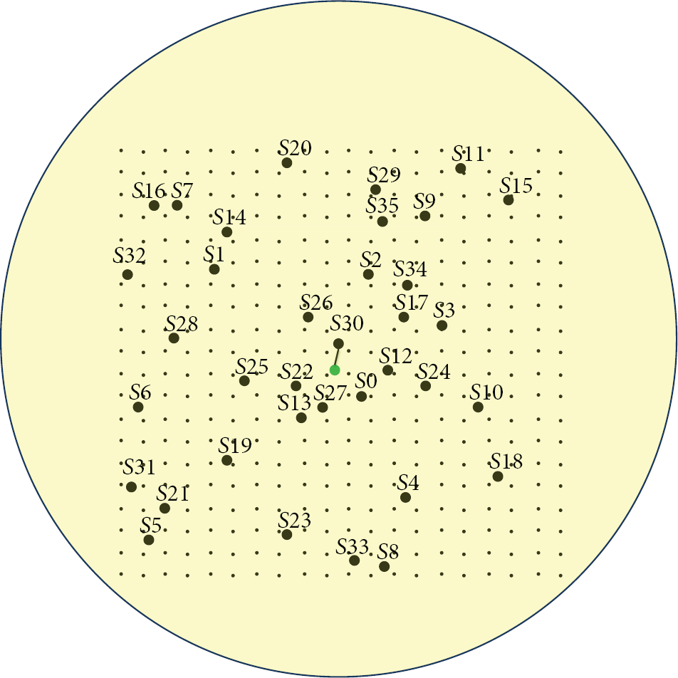
A demand point is a geographical point in the region of monitoring where one or more phenomena are sensed. The distribution of such points across the area of monitoring can be regular, like a grid, but can also be random in nature. The density of such points varies according to the spatial phenomenon's variation under observation. At least one sensor must be active in a given moment to sense each demand point. Such constraint is implemented in the model.

(2)

Usually, the sensors are associated with coverage areas that cannot be estimated accurately. To simplify the modelling, we assume plain areas without obstacles. Moreover, we assume a circular coverage area. The coverage radius is determined by the spatial variation of the sensed phenomenon. It is assumed that all demand points within this area can be sensed. The radio-frequency propagation in real WSNs is also irregular in nature. In the same way, we can assume a circular communication area. The radius of this circle is the maximum distance at which two sensor nodes can interact.

(3)

A route is a path from one sensor node to a sink possibly passing through one or more sensor nodes by retransmission. Gateways are regarded as special sensor nodes whose role is only to interface with the sinks. Each phenomenon sensed in a node has its data associated with a route leading to a given sink, which is independent from the routes followed by the data related to other phenomena sensed in the same sensor node.

(4)

The energy consumption is actually the electric current drawn by a circuit in a given time period.

In what follows [11, 13–16], the constants, variables, objective function, and constraints of the integer linear programming model applied energy consumption in heterogeneous are introduced in a step-by-step manner.

3.1. Constants

$S$ :

set of sensors;

D :

set of demand points;

M :

set of sinks;

T :

set of n scheduling periods;

G :

set of phenomena (temperature, humidity, barometric pressure, etc.). Each phenomenon has its own spatio-temporal properties. The associated sampling rate has impact on data traffic, while the associated radius of coverage has impact on the number of active sensors;

$A_{i j}$ :

set of arcs $i j$ , $i \in S$ , $j \in D$ , link sensors to demand points;

${E B}_{i}$ :

cumulated battery energy for sensor $i \in S$ ;

${E A}_{i}$ :

energy dissipated while activating sensor $i \in S$ ;

${E M}_{i}$ :

energy dissipated while sensor $i \in S$ is activated (effectively sensing);

${E T}_{i j}^{g}$ :

energy dissipated when transmitting data from sensor i to sensor j with respect to phenomenon g. Such values can be different for each arc $i j$ if a sensor can have its transmitter power adjusted based on the distance to the destination sensor. Each phenomenon has its own sampling rate, a parameter that impacts the total amount of data transmitted across the WSN and, consequently, the levels of energy waste;

${E R}_{i}$ :

energy expended in the reception of data for sensor $i \in S$ ;

${E H}_{j}^{g}$ :

penalty applied when any sensor does not cover a demand point $j \in D$ for phenomenon g;

${E G}_{i}^{g}$ :

penalty applied when sensor $i \in S$ is activated to unnecessarily sense the phenomenon g;

${A D}_{s d}^{g}$ :

set of arcs indicates whether the sensor s coppers the point of demand d for phenomenon g.

3.2. Variables

These are the decision variables:

$w_{i}^{t} {0,1}$ :

if sensor i was activated in period t for at least one phenomenon;

$y_{i}^{t} \in {0,1}$ :

if sensor i is activated in period t;

$x_{i j}^{t g} \in {0,1}$ :

if sensor i covers demand point j in period t for phenomenon g;

$z_{l i j}^{t g} \in {0,1}$ :

if arc $i j$ belongs to the route from sensor l to a sink in period t for phenomenon g;

$r_{i}^{t g} \in {0,1}$ :

if sensor i was activated in period t for phenomenon g;

$h_{j}^{t g} \in {0,1}$ :

if demand point j for phenomenon g is not covered by any sensor in time period t;

$e_{i}$ :

Energy consumed by sensor i considering all time periods.

3.3. Objective Function

The objective function (1) minimizes the total energy consumption through all time periods. The second term penalizes the existence of some uncovered demand points, but the solution continues feasible. It penalizes unnecessary activation for the phenomenon too.

Consider:

\begin{matrix} \min \sum_{i \in S} e_{i} + \sum_{t \in T} \sum_{g \in G} \sum_{j \in D} {E H}_{j}^{t} h_{j}^{t g} . \end{matrix}

(1)

3.4. Restrictions

The constraint (2) enforces the activation of at least one sensor node i to cover the demand point j associated with phenomenon g in period t. Otherwise, the penalty variable $h_{j}^{t g}$ is set to one. This last condition will occur only in those cases when there is no sensor node that can cover the demand point, that is, for the lack of battery power when being used for other time periods and/or to monitor other phenomena, or because there is no sensor that can cover the demand point

\begin{matrix} \sum_{s \in S} {A D}_{s d}^{g} x_{s j}^{t g} + h_{j}^{t g} \geq 1, \forall j \in D, \forall t \in T, \forall g \in G . \end{matrix}

(2)

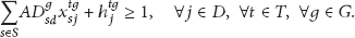
Figure 3 illustrates the results of two time intervals fourth sensor nodes. The corresponding indices are

(i)

time interval = 0;

(ii)

sensor = 0;

(iii)

measure = 0;

(iv)

demand point 21.

Figure 3

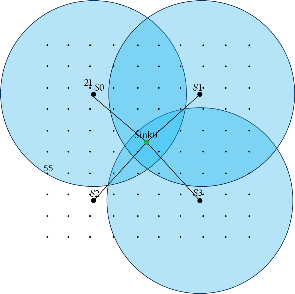
The application of the covering according to the chosen variable $x_{i j}^{t g}$ .

The $A D$ constant for the indices quoted indicates that it is possible to cover the demand point 0 by the sensor 21, in the time interval 0 to 0 magnitude. If this sensor is selected to satisfy the constraint, the corresponding value of $x_{i j}^{t g}$ is equal to 1. If no sensor is allocated to cover a demand point, which happens for example with the demand point 55, wherein the sensor 2 is the only sensor that can monitor it and is not active, then the variable $x_{i j}^{t g}$ for the corresponding index value will be equal to 0, and the variable $h_{j}^{t g}$ equals 1, and the penalty is applied.

On the other hand, the constraint (3) turns on variable $r_{i}^{t g}$ (which means that a sensor node is actively sensing phenomenon g in period t) if its associated sensor node is indeed allocated to cover any demand point associated with g. Furthermore, the variable $r_{i}^{t g}$ is applied in an other restriction of connectivity to indicate the start of the route if the sensor node is active.

Consider:

\begin{matrix} x_{t s}^{d g} \leq r_{s}^{t g}, \forall d \in D, \forall s \in S, \forall g \in G, \forall t \in T . \end{matrix}

(3)

Besides, the constraint (4) reads that sensor node i is fully active (parameter $y_{s}^{t}$ ) if it is active for at least one phenomenon of observation. This constraint is used to facilitate the implementation of energy maintenance, and the activation sensor for routing restrictions is described,

\begin{matrix} r_{s}^{t g} \leq y_{s}^{t}, \forall t \in T, \forall g \in G, \forall s \in S . \end{matrix}

(4)

In restriction (5), an exit route exists for a sensor node j to node k sensor if there is already a path of arrival sensor node i to node j sensor at time interval t, the phenomenon g. The constant $A_{i j}$ indicates whether a sensor has a connectivity with another sensor. The index l indicates the sensor node that initiated the route,

\begin{matrix} \sum_{\begin{matrix} i \in S \\ i \neq j \end{matrix}} A_{i j} z_{l i j}^{t g} - \sum_{\begin{matrix} k \in S \cup M \\ i \neq j \end{matrix}} A_{j k} z_{l j k}^{t g}, \forall j, l \in S, \forall g \in G, \forall t \in T . \end{matrix}

(5)

In Figure 4, if an input arc $i j$ (s3, s6), for example, will have to be some other output arc, for example, $j k$ (s6, sin $k 0$ ), that is, $z_{l s 3 s 6}^{t g} - z_{l s 6 \sin k 0}^{t g} = 0$ , the sum is applied to indicate all possible routes according to the constant connectivity of the time interval t and magnitude g. The index l indicates the node that initiated the route.

Figure 4

Applying connectivity according to the chosen variable $z_{l i j}^{t g}$ .

Moreover, in restriction (6) if a node is active, then there must be a route starting from it. As previously mentioned, the variable r indicates whether a sensor node s is active at a time t, g for measure. This restriction is necessary because it is the beginning of the route, or one route out, not being possible to be met by the conservation flow.

Consider:

\begin{matrix} \sum_{k \in S \cup M} A_{i k} z_{l i k}^{t g} = r_{i}^{t g}, \forall l, i \in S, \forall g \in G, \forall t \in T . \end{matrix}

(6)

And also in constraint (7), if a sensor node is active, then its route must end in a sink node. Similarly to the previous restriction (6), it is not possible to apply the conservation flow since there is no exit route for sink node, only income,

\begin{matrix} \sum_{i \in S} \sum_{j \in M} A_{l k} z_{l i k}^{t g} = r_{l}^{t g}, \forall l \in S, \forall g \in G, \forall t \in T . \end{matrix}

(7)

Furthermore, constraint (8) indicates that if there is an exit route past a sensor node, the sensor node must be active. A sensor node can be active only for data transmission, then the decision variable $y_{i}^{t}$ indicates that it should be active to receive value equal to the greater presence of the exit route,

\begin{matrix} A_{i j} z_{l i j}^{t g} \leq y_{i}^{t}, \forall l, i \in S, \forall g \in G, \forall t \in T, \forall j \in S \cup M . \end{matrix}

(8)

Constraint (9) shows that if there is an entry of a route that passes by a sensor node, then that sensor node must be active. In the same way, for the constraint of output going the route of input

\begin{array}{l} A_{i j} z_{l i j}^{t g} \leq y_{j}^{t}, \forall l, i \in S, \forall g \in G, \forall t \in T, \forall j \in S \cup M, \\ with i \neq j, l \neq j . \end{array}

(9)

Constraint (10) determines the total energy spent by sensors throughout the time that the network is active:

(a)

it is added for each sensor i, and the energy is expended in all periods of time with maintenance $(E M_{i} y_{i}^{t})$ , if $y_{i}^{t} = 1$ ;

(b)

the same happens with the activation of sensors indicated by the variable $w_{i}^{t}$ , with $E A_{i} w_{i}^{t}$ .

All the energy for receiving data from the sensor l, although not itself, who comes from sensor k, is added in $\sum_{l \in S}^{l \neq i} \sum_{k \in S} \sum_{g \in G} {E R}_{l} A_{k i} z_{l k i}^{t g}$ .

The same happens with the energy that used to transmit data, except that it may be the sensor that initiated the route expressed by this part, $\sum_{l \in S} \sum_{j \in S \cup M} \sum_{g \in G} {E T}_{g}^{i j} A_{i j} z_{l i j}^{t g}$ .

Therefore,

\begin{array}{l} \sum_{t \in T} ({E M}_{i} y_{i}^{t} + {E A}_{i} w_{i}^{t} + \sum_{l \in S}^{l \neq i} \sum_{k \in S} \sum_{g \in G} {E R}_{i} A_{k i} z_{l k i}^{t g} \\ + \sum_{l \in S} \sum_{j \in S \cup M} \sum_{g \in G} {E T}_{g}^{i j} A_{i j} z_{l i j}^{t g}) \leq e_{i}, \forall i \in S . \end{array}

(10)

Constraint (11) enforces that each sensor node should consume at most the capacity limit of its battery,

\begin{matrix} 0 \leq e_{i} \leq {E B}_{i}, \forall i \in S . \end{matrix}

(11)

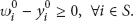
If a sensor is active in the first time interval, it means it consumed energy to activate. The w variable indicates this activation. Then, the variable's value is set to 1. On the other hand, if the sensor is kept off in the first time interval, the value is set to 0. Constraint (12) ensures that

\begin{matrix} w_{i}^{0} - y_{i}^{0} \geq 0, \forall i \in S . \end{matrix}

(12)

In constraint (13), the sensor's past and current activation states are compared. If the sensor node was active from period $t - 1$ to period t, then w is set to 1 or 0, otherwise,

\begin{matrix} w_{i}^{t} - y_{i}^{t} + y_{i}^{t - 1} \geq 0, \forall i \in S, \forall t \in T, t > 0 . \end{matrix}

(13)

4. Computational Results

The following conditions were considered to execute the computational tests: four different scenarios are set according to the time interval amounts 2, 4, 6, and 8 time intervals. For each time interval, it was executed for some instances using only phenomenon light and, other instances using two phenomena: temperature and light. The sensor's coverage radius used for temperature was 8.8 meters, and light used a coverage radius of 16 meters. The connectivity radius among the sensors is set to 11 meters. A regular grid of demand points with 400 points was distributed in a square area of $10 \times 10$ meters, with four demand points per m². Each demand point may be associated with a phenomenon, but the coverage of the sensors is totally independent of a demand point alone. Likewise, 36 sensors were distributed in a regular grid of $6 \times 6$ over the monitoring region, and in other instances, distributed randomly. All sensor nodes have the same characteristics as the coverage capacity, processing, and transmission. Only one sink node was used, allocated in the center the monitored region. All elements of described (demand points, sensors, and sinks) were generated applying geographic coordinates.

The constants energy values were calculated according to the values found in the manufacturer's sensor manual (Mote battery life calculator). The total transmission and reception data in a given time interval are calculated based on the amount of data and rate adopted by the devices. A constant representing the penalty for not covering a demand point is assigned for a value considerably high to force the model to find a result that meets all coverage restrictions.

In [1, 3, 17, 18] they conceived their computational experiments to produce WSNs with the minimum energy consumption as possible, while maintaining the coverage and connectivity constraints. The gain obtained in their work is calculated by the comparison of the minimum set of sensors that have to be active and the energy waste caused by the activation of all sensors with high coverage overlapping in a high density configuration [4].

The Integer Linear Programming (ILP) [19] model was implemented in the programming language Java 6 using the library Concert22, responsible for integrating the solver used. The tests’ cases were solved by the IBM dynamic library integrated CPLEX12.1 (IBM ILOG CPLEX). The machine used on this test was an Intel i7 64 bits with 8 GB of RAM with windows 7 64 bits [20].

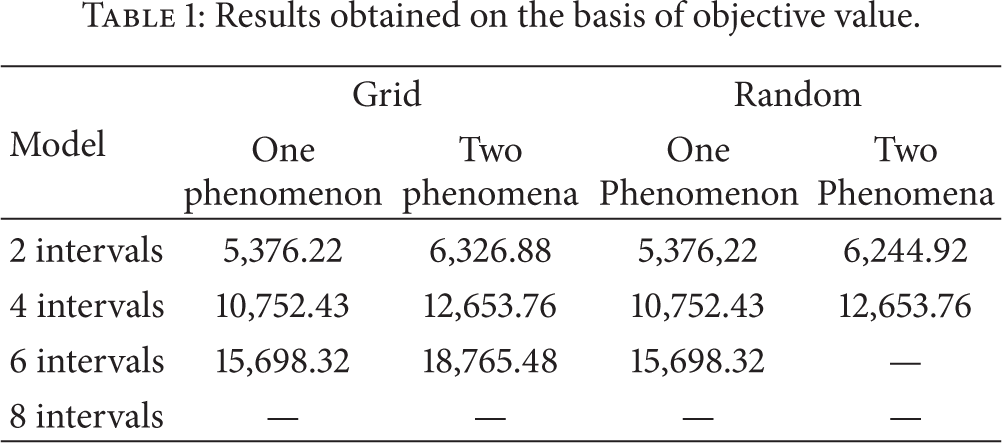
Table 1 shows the results obtained by running the model for heterogeneous networks using one and two phenomena, both for sensors allocated in grid and randomly, with the objective's function values composed of two parts: the electrical charge summation consumption in all sensor nodes and the penalties. The penalties are an artifact that allows the model to remain feasible even when some demand points are not covered by any sensor, giving flexibility to the model, but at the same time this resource must be well calibrated to avoid its unnecessary use that would cause disturbance in the real solution. Thus, the real objective is calculated by subtracting the artificial coverage penalties of the objective function or just calculating the first part (summation) of the objective expression.

Table 1

Results obtained on the basis of objective value.

Model	Grid		Random
Model	One phenomenon	Two phenomena	One Phenomenon	Two Phenomena
2 intervals	5,376.22	6,326.88	5,376,22	6,244.92
4 intervals	10,752.43	12,653.76	10,752.43	12,653.76
6 intervals	15,698.32	18,765.48	15,698.32	—
8 intervals	—	—	—	—

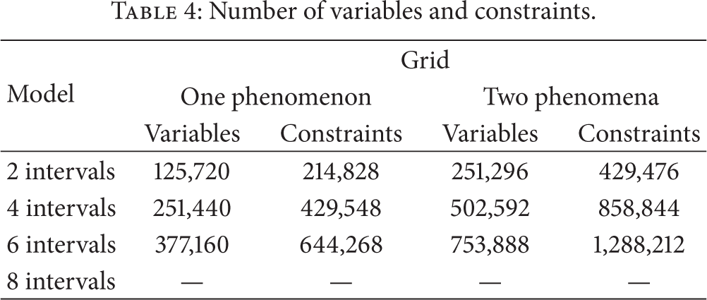
In these experiments, the demand points are disposed in a grid and randomly. In Table 2, the values are in function of execution time represented in minutes: seconds, distributed analogously to Table 1. Analogously to Tables 1 and 2, Table 3 values represent the noncovered demand points’ percentage (%). Table 4 represents the number of variables and constraints of the problem when the exact method is applied. For both grid and random allocations, the number of constraints and variables is the same for each characteristic. This equality is due to the same problem; just the data about coverage and connectivity are changed.

Table 2

Results obtained in the light of the runtime (minutes : seconds).

Model	Grid		Random
Model	One phenomenon	Two phenomena	One Phenomenon	Two Phenomena
2 intervals	0 : 13	1 : 32	0 : 21	1 : 13
4 intervals	0 : 50	10 : 32	0 : 57	24 : 34
6 intervals	1 : 08	937 : 04	15 : 12	—
8 intervals	—	—	—	—

Table 3

Results obtained based on demand points.

Model	Grid		Random
Model	One phenomenon	Two phenomena	One phenomenon	Two phenomena
2 intervals	0.00%	0.00%	0.00%	0.00%
4 intervals	0.00%	0.00%	0.00%	0.00%
6 intervals	0.00%	0.00%	0.00%	—
8 intervals	—	—	—	—

Table 4

Number of variables and constraints.

Model	Grid
	One phenomenon		Two phenomena
	Variables	Constraints	Variables	Constraints
2 intervals	125,720	214,828	251,296	429,476
4 intervals	251,440	429,548	502,592	858,844
6 intervals	377,160	644,268	753,888	1,288,212
8 intervals	—	—	—	—

The real purpose of this model is to extend the WSN lifetime as far as possible, reducing the WSN energy cost and preserving its coverage and connectivity. So, lower electrical charge consumption is not necessarily an important issue if it does not reflect on more time slots. The number of time slots multiplied by the duration of the time slot represents the WSN lifetime. This idea seems coherent at first glance since energy waste reduction is often desirable.

The only drawback here is the uncovered demand point rate, which is worse than ILP value. Despite this small imperfection, many real applications tolerate some lack of coverage by the nature of the observed phenomenon and other aspects. Even though, this uncovered demand points are often situated at the periphery of the observed area. The coverage radius does not reflect necessarily a sharp threshold of sensing. The implementation of heterogeneous networks by applying exact method for scenarios with 8 time intervals increased in size so as not to allow the solver to find the solution within 24 hours.

Analysing the results, it is observed that the heterogeneous network has an energy saving, considering that the phenomena are handled differently. The radio of coverage for the phenomena is different, making it unnecessary to monitor a given phenomenon, in this case light, by having a greater radius of coverage by various sensors, reducing the amount of redundant data to be transmitted.

Figure 5 shows the result obtained for an implementation of a WSN with six time intervals, 36 sensor nodes, 400 demand points, and two phenomena. For the temperature phenomenon, in the time intervals 2 and 4, the network's configuration is given in Figure 5.

Figure 5

The time intervals 6 and 8 configurations are given by Figure 6. The configuration is able to maintain the network active in the three given periods, so it is not necessary to change the network's configuration in the time given.

Figure 6

The same happens with the light phenomenon, but for the time intervals 2, 4, 6, and 8, shown by Figure 7, the configuration is the same. This happens because the coverage radius is big enough to only be capable to cover the entire sensoring area, and the necessary energy to transmit the data is less than temperature. The time interval 6 needed another configuration, as the previous sensor's battery energy would not be enough to maintain the network active. This last configuration is shown in Figure 8.

Figure 7

Figure 8

5. Conclusion and Future Works

The difference between the homogeneous [11] and the heterogeneous is that the last one has the capacity to deal with different phenomena independently, giving different sample data and sensed range for each phenomenon. This implies in a different way to treat the network's transmission data. Although it does not implement any density explosion control, good solutions are found in feasible execution time for wireless sensor network that could not be possible if only ILP was applied.

The results found are far better than the reference literature and leave opportunities for future enhancements as new supplementary algorithms and heuristics are aggregated to this methodology [21–24].

Another promising line of investigation involves the design and implementation of parallel/distributed versions of the framework, by means of which several GRI (Generator of reduced instances) and SRI (solver of reduced instances) instances could run concurrently, each one configured to explore different aspects of the optimization problem at hand. The use of insular genetic algorithms [25–28] can bring more diversity and possibilities, resulting in effectiveness enhancement. Moreover, other metaheuristics such as particle swarm could be experimented replacing or working cooperatively with genetic algorithms.

This hybrid methodology can be adapted to tackle other problem classes like WSN as shown here. The key point in this adaptation is finding the best or at least a good reducible structure. This analysis is very linked to the chromosome encoding choice as it represents a trade of between subproblem complexity range width and chromosome size. A good reducible structure allows a wide range of subproblem complexity from very light and fast subproblems to the actual real problem. On the other hand, the reducible matrix size, affects the chromosome size and a large chromosome size reduces the GA effectiveness.

The dynamic coverage and connectivity in wireless sensor networks’ problem applied are a very different problem class than the cutting and packing class used in the original version [29–32]. In this problem, a good reducible structure was found but it is much larger than the ones found in the cutting and packing problem instance. That is, the reason why a new chromosome encoding was developed. This new encoding makes the matrix choice viable.

Moreover, the publication of some papers related to this subject [33] brought a good understanding about how to give new contributions to this area and present better solutions. According to [13], experiments were made for the dynamic coverage and connectivity in wireless sensor networks’ problem using what is mentioned in Section 3. The use of integer linear programming approach is limited to a certain level of complexity that sometimes is not enough for a real size network (Table 4). It is expected that other hybrid methodologies [15, 34] can be applied in the solution of the problem.

Footnotes

Acknowledgments

The first author is thankful to the National Council of Technological and Scientific Development (CNPq) via Grant no.305844/2011-3, the second author is thankful to the “Foundation for Support of Scientific and Technological Development Ceara State” (FUNCAP) for Grant no. PRN-0040-00037.01.00/10, and the third author is thankful to the “Coordination for the Improvement of Higher Personnel” (CAPES) for the support received on this project. The authors also acknowledge IBM for making the IBM ILOG CPLEX Optimization Studio available to the academic community.

References

Nakamura

F. G.

Mateus

G. R.

Planejamento dinâmico para controle de cobertura e conectividade em redes de sensores sem fio

Workshop de Comunicação sem Fio e Computação Móvel

2004

182 191

Martins

F. V. C.

Nakamura

F. G.

Quintão

F. P.

Mateus

G. R.

Model and algorithms for the density, coverage and connectivity control problem in flat WSNs

Proceedings of the International Network Optimization Conference

2007

Quintão

F. P.

Nakamura

F. G.

Mateus

G. R.

A hybrid approach to solve the coverage and connectivity problem in wireless sensor networks

Proceedings of the 4th European Workshop on Metaheuristics: Design and Evaluation of Advanced Hybrid Metaheuristics

2004

Nottingham, UK

de Aguiar

A. B.

Neto

A. M. S.

Cunha

R. P. P.

Pinheiro

P. R.

Coelho

A. L. V.

A hybrid methodology for coverage and connectivity in wireless sensor network dynamic planning

41st Simpósio Brasileiro de Pesquisa Operacional

2010

Bento Gonçalves, Brazil

Zhou

Liang

Xie

Multiobjective coverage control strategy for energy-efficient wireless sensor networks

International Journal of Distributed Sensor Networks 2012 2012 10

720734

10.1155/2012/720734

Quintão

F. P.

Nakamura

F. G.

Mateus

G. R.

Evolutionary algorithm for the dynamic coverage problem applied to wireless sensor networks design

Proceedings of the IEEE Congress on Evolutionary Computation (IEEE CEC ′05)

September 2005

1589 1596

2-s2.0-27144530235

Ishebabi

Mahr

Bobda

Gebser

Schaub

Answer set versus integer linear programming for automatic synthesis of multiprocessor systems from real-time parallel programs

International Journal of Reconfigurable Computing 2009 2009 11

863630

10.1155/2009/863630

Nguyen

Cheung

S. C.

On reducing communication energy using cross-sensor coding technique

International Journal of Distributed Sensor Networks 2011 2011 12

2-s2.0-79955034759

10.1155/2011/837128

837128

Megerian

Koushanfar

Veltri

Potkonjak

Exposure in wireless sensor networks: theory and practical solutions

Wireless Networks 2002 8 5 443 454

2-s2.0-0036738161

10.1023/A:1016586011473

10.

Megerian

Potkonjak

Lower power 0/1 coverage and scheduling techniques in sensor networks

2003 030001

University of California, Los Angeles

11.

Pinheiro

P. R.

Coelho

A. L. V.

de Aguiar

A. B.

Neto

A. M. S.

Towards aid by generate and solve methodology: applying in the problem of coverage and connectivity in wireless sensor networks

International Journal of Distributed Sensor Networks 2012 2012 11

790459

10.1155/2012/790459

12.

Wang

Xing

Zhang

Pless

Gill

Integrated coverage and connectivity configuration in wireless sensor networks

Proceedings of the 1st International Conference on Embedded Networked Sensor Systems (SenSys ′03)

November 2003

New York, NY, USA

ACM

28 39

2-s2.0-18844371448

13.

de Aguiar

A. B.

Pinheiro

P. R.

Coelho

A. L. V.

Neto

A. S.

Cunha

R. P. P.

Scalability analysis of a novel integer programming model to deal with energy consumption in heterogeneous wireless sensor networks

Communications in Computer and Information Science 2008 14 11 20

10.1007/978-3-540-87477-5_2

14.

de Aguiar

A. B.

Pinheiro

P. R.

Coelho

A. L. V.

Optimizing energy consumption in heterogeneous wireless sensor networks: a novel integer programming model

Proceedings of the 4th International Conference on Operational Research for Development (ICORD ′07)

2007

496 505

15.

de Aguiar

A. B.

Pinheiro

P. R.

Coelho

A. L. V.

Bonates

T. O.

On the concept of density control and its application to a hybrid optimization framework: investigation into cutting problems

Computers and Industrial Engineering 2011 61 3 463 472

2-s2.0-80053211044

10.1016/j.cie.2011.03.013

16.

Pinheiro

P. R.

Coelho

A. L. V.

de Aguiar

A. B.

Neto

A. M. S.

Applying the generate and solve methodology in the problem of dynamic coverage and connectivity in wireless sensor networks

Proceedings of the Information Science and Industrial Applications (ISI ′12)

2012

Cebu, Philippines

SERSC

252 257

17.

de Andrade

I. B. D.

Mateus

G. R.

Nakamura

F. G.

A GRASP heuristic to density control: solving multi-period coverage and routing problems in wireless sensor networks

Proceedings of the IEEE Symposium on Computers and Communications (ISCC ′09)

July 2009

Sousse, Tunisia

493 499

2-s2.0-70449507257

10.1109/ISCC.2009.5202370

18.

de Aguiar

A. B.

Tackling the problem of dynamic coverage and connectivity in wireless sensor networks with an extended version of the generate and solve methodology generate and solve methodology [M.S. thesis] 2009

Graduate Program in Applied Informatics, University of Fortaleza

19.

Wolsey

L. A.

Integer Programming 1998

New York, NY, USA

John Wiley & Sons

20.

ILOG

I. B. M.

ILOG CPLEX 12.0 User's Manual

2011

21.

Blum

Roli

Metaheuristics in combinatorial optimization: overview and conceptual comparison

ACM Computing Surveys 2003 35 3 268 308

2-s2.0-0344236266

10.1145/937503.937505

22.

Dumitrescu

Stützle

Combinations of local search and exact algorithms

Applications of Evolutionary Computing 2003 2611

New York, NY, USA

Springer

211 224 Lecture Notes in Computer Science

23.

Eiben

A. E.

Smith

J. E.

Introduction to Evolutionary Computing 2003

New York, NY, USA

Springer

24.

Talbi

E. G.

A taxonomy of hybrid metaheuristics

Journal of Heuristics 2002 8 5 541 564

2-s2.0-0036723306

10.1023/A:1016540724870

25.

Jonatã

Araújo

Pinheiro

P. R.

Applying backtracking heuristics for constrained two-dimensional Guillotine cutting problems

Information Computing and Applications 2011 7030

New York, NY, USA

Springer

113 120 Lecture Notes in Computer Science

2-s2.0-83755206144

10.1007/978-3-642-25255-6_15

26.

Saraiva

R. D.

Pinheiro

P. R.

A novel application of crossover operator to a hybrid optimization framework: investigation into cutting problems

Proceedings of the IEEE Congress on Evolutionary Computation

2012

633 639

27.

Saraiva

R. D.

Nepomuceno

N. V.

Pinheiro

P. R.

Middendorf

Blum

The generate-and-solve framework revisited: generating by simulated annealing

Evolutionary Computation in Combinatorial Optimization 2013 7832

New York, NY, USA

Springer

262 273 Lecture Notes in Computer Science

28.

de Araújo

L. J. P.

Pinheiro

P. R.

Heuristics backtracking and a typical genetic algorithm for the container loading problem with weight distribution

Communications in Computer and Information Science 2010 106 2 252 259

2-s2.0-78649404975

10.1007/978-3-642-16339-5_33

29.

Nepomuceno

N. V.

Pinheiro

P. R.

Coelho

A. L. V.

Tackling the container loading problem: a hybrid approach based on integer linear programming and genetic algorithms

Evolutionary Computation in Combinatorial Optimization 2007 4446

New York, NY, USA

Springer

154 165 Lecture Notes in Computer Science

2-s2.0-38049079262

30.

Nepomuceno

N. V.

Pinheiro

P. R.

Coelho

A. L. V.

Cotta

van Hemert

A hybrid optimization framework for cutting and packing problems: case study on constrained 2D non-guillotine cutting

Recent Advances in Evolutionary Computation for Combinatorial Optimization 2008 153 87 99

31.

Puchinger

Raidl

G. R.

Combining metaheuristics and exact algorithms in combinatorial optimization: a survey and classification

Lecture Notes in Computer Science

Proceedings of the 1st International Work-Conference on the Interplay between Natural and Artificial Computation (IWINAC ′05)

June 2005

41 53 Lecture Notes in Computer Science

2-s2.0-26444552169

32.

Araújo

L. J. P.

Pinheiro

P. R.

Combining heuristics backtracking and genetic algorithm to solve the container loading problerm with weight distribution

Advances in Intelligent and Soft Computing 2010 73 95 102

33.

de Aguiar

A. B.

Neto

A. M. S.

Pinheiro

P. R.

Coelho

A. L. V.

Applicability of a novel integer programming model for wireless sensor networks

International Journal of Computer Science and Information Security 2009 3 1 7 13

34.

Pinheiro

P. R.

Oliveira

P. R.

A hybrid approach of bundle and benders applied large mixed linear integer problem

Journal of Applied Mathematics 2013 2013 11

678783

10.1155/2013/678783

Handing Optimization Energy Consumption in Heterogeneous Wireless Sensor Networks

Abstract

1. Introduction

2. The Wireless Sensor Network

3. The Integer Linear Programming Model

3.1. Constants

3.2. Variables

3.3. Objective Function

3.4. Restrictions

4. Computational Results

5. Conclusion and Future Works

Footnotes

Acknowledgments

References