Cooperative Processing Model for Wireless Sensor Networks

Abstract

Wireless sensor networks offer a distributed processing environment. Many sensor nodes are deployed in fields that have limited resources such as computing power, network bandwidth, and electric power. The sensor nodes construct their own networks automatically, and the collected data are sent to the sink node. In these traditional wireless sensor networks, network congestion due to packet flooding through the networks shortens the network life time. Clustering or in-network technologies help reduce packet flooding in the networks. Many studies have focused on saving energy in the sensor nodes because the limited available power leads to an important problem of extending the operation of sensor networks as long as possible. However, we focus on the execution time because clustering and local distributed processing already contribute to saving energy by local decision making. In this paper, we present a cooperative processing model based on the processing timeline. Our processing model includes validation of the processing, prediction of the total execution time, and determination of the optimal number of processing nodes for distributed processing in wireless sensor networks. The experiments demonstrate the accuracy of the proposed model, and a case study shows that our model can be used for the distributed application.

1. Introduction

Wireless sensor networks are generally composed of sensor nodes capable of detecting, processing, and transmitting. Sensor nodes collect environmental data, such as temperature, humidity, sound, vibration, or magnetic field strength, and send information that is processed from the collected data to the sink or base station. The data collected from the sensors are converted to digital data via analog-to-digital converters, and the sensor node identifies surrounding information, for example, object location or environmental event. The environmental information is used for forecasting certain events, monitoring disasters such as earthquakes and forest fires, or military purposes.

The traditional wireless sensor networks have been designed such that an external computing system makes decisions with data from the base station. The network lifetime in this type of architecture decreases because of relaying packets on the network and shrinks dramatically around the base station. Over the past decades, various methods to solve this problem have been studied based on distributing and sharing process resources. Distributed in-network processing can increase network lifetime and decrease the response time for events [1, 2].

The various wireless sensor network applications, such as tracking objects, detecting intruders, and monitoring structural health, generate many data packets on networks. Distributed processing or in-network processing reduces the number of packets to the base station by extracting information from measured raw data. More energy is required for transmitting and receiving data via radio frequency than for sensing and processing. Reducing packets into the network contributes to increasing network lifetime because it removes packet duplication caused by relaying packets to the base station [3].

Wireless sensor networks have different features from existing computing environments. A sensor node is small and has low computing power and very limited wireless bandwidth. Hence, the total execution time for distributed processing is affected by the data size and transmission rate. In particular, the low bandwidth of ZigBee that is used in a well-known sensor mote, such as MICAz of the University of California, Berkeley, affects the total execution time [4].

The energy efficiency and fairness of a network has been considered an important subject in the existing research concerning distributed or in-network processing. The execution time of the distributed processing has received little attention, though it is important to design energy-efficient sensor network applications. In this paper, we will focus on the total execution time estimation of processing and how to determine the optimal number of processing nodes based on a proposed estimation method in a low-bandwidth wireless network [5].

In Section 2, we describe clustered wireless sensor networks which bring the benefits in response time and energy consumption. Our proposed processing model is described in Section 3. In the network model we studied, how to validate it based on total execution time, the total execution time estimation model, and the cluster size for optimization of the execution time are discussed. We evaluate the accuracy of our estimation model in the experiment with the MICAz sensor mote in Section 4. A case study using a fast Fourier transform is presented in Section 5. Finally, we conclude the paper in Section 6.

2. Cluster in Wireless Sensor Network

Wireless sensor networks take the role of a bridge between the real world and the computing world. Distributed measurements are used in various areas including environmental monitoring, vehicle detection for transportation, detection of disaster, industrial safety management, military operation, and smart spaces [6].

Most sensor network applications need to be real time. Figure 1 shows the value changes according to time of a task with deadline D in real-time systems. If the detected data are not processed on time, the value of the processed results will decrease in a soft real-time system of Figure 1(a) and become zero in a hard real-time system of Figure 1(b). If the processing delay affects safety, the value of the results can be negative such as Figure 1(c) [7].

Figure 1

Value changes according to time.

Consider the sensor network application that detects an intrusion and takes a video of the area. Sensor nodes report to the sink node whenever a movement of a human, an animal, or some kind of object is detected, and the sink node decides whether it is an intruder based on the reported raw data. If the movement is identified as an intruder, the sink node sends the action command. The actions can be turning on a camera and taking a video. If the sink node takes action after the object has moved out of the area, the camera would not be able to record a video of the detected object [8].

Similarly, a structural health monitoring application checks the vibration frequency for detecting structural damage such as cracks. The collected vibration data are sent to the sink node, which analyzes the vibrations with signal processing techniques such as a Fourier transform. If structural damage is detected, the sink node should take action to alert the structural management system. However, if it takes a long time to relay data to the sink node, the action cannot be executed on time.

As described earlier, the real-time property is important for many wireless sensor network applications. However, it is difficult to obtain a fast real-time system. It may be impossible in some cases because the sensor nodes typically have insufficient resources and are deployed in harsh environments occasionally. Clustering techniques can be a solution for these wireless sensor network applications. The distributed processing or in-network processing of a cluster does not report all raw data. Instead, the node that has raw data processes data with neighbor nodes cooperatively.

The process of reporting data to the sink node suffers from not only end-to-end delay by multihop communication but also greater energy consumption in particular cases. The research [9] compared the performance of nonclustered and clustered sensor networks. They evaluated two types of “bit-hop metrics,” which count the total number of bit transmissions in the network ( $\text{BT}$ ). Their equations are summarized as follows:

$$\begin{array}{cc}& E=E_T+E_R=\text{BT}\left(E_{T\text{-bit}}+E_{R\text{-bit}}\right),\end{array}$$

(1)

where E is the total energy consumption by transmission, $E_T$ and $E_R$ are the energy costs by sending and receiving one bit of data, respectively, and $E_{T\text{-bit}}$ and $E_{R\text{-bit}}$ are the energy consumed for transmitting and receiving one bit of data, respectively. They assumed that there are Q sensor nodes in the network, the cluster size is c, and α is the average factor of in-cluster data reduction per each reported reading. Finally, they created the following equation:

$$\begin{array}{cc}& {\text{BT}}_{\text{clustered}}<{\text{BT}}_{\text{non-clustered}}⟺\frac{Q-c}{\sqrt{c}}+\alpha ·Q<c.\end{array}$$

(2)

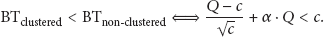
From (2), we find the fact that the ability of clustered wireless sensor networks to outperform their nonclustered counterparts is conditioned by the values of Q, c, and α. Furthermore, they discussed two special cases, that is, $\alpha =c/Q$ and $\alpha =1$ , and derived the conclusion that the degree of correlation between readings of intercluster nodes must be quite high to ensure full performance superiority of clustered over nonclustered wireless sensor networks. On the other hand, if correlation between the nodes’ readings is very low or there is no correlation, the utilization of node clustering should be avoided.

In order to obtain high performance from clustered wireless sensor networks, the value of correlation α should be high. If α is controllable, the performance efficiency of clustering can be improved. In the research [9], the cluster head ( $\text{CH}$ ) aggregates data from the cluster member nodes based on spatial locality. We consider a different clustering model. The $\text{CH}$ does not aggregate data but processes data with cluster member nodes cooperatively. The details are described in Section 3.

The local distributed processing model with clustering proposed in this paper can be an alternative to control α for improvement of the network performance in terms of energy consumption. In this model, the $\text{CH}$ only has data; thus, the correlation of readings can be regarded to be very high so that the performance of clustered networks is guaranteed to be superior to the performance of nonclustered wireless sensor networks.

3. Cooperative Processing Model

3.1. Network Model

Wireless sensor nodes have very limited resources, including computing power, memory, and network bandwidth. This is a considerable difference between the distributed in-network processing of wireless sensor networks and the existing computing environments. In particular, we should consider low network bandwidth when designing in-network processing applications. According to the data size, distributed processing could be slower than execution on a node.

We consider a distributed processing model in a cluster in a wireless sensor network, which is composed of a root node that has data to be processed and n processing nodes that process divided data from the root node. We assume the following statements to simplify our execution time estimation model.

• (i)

  The root node and processing nodes are located at the one-hop distance for direct communication.

• (ii)

  Transmission errors are not considered. It is assumed that the handling of transmission errors is performed at the sublayers of communication stack.

• (iii)

  The root node transmits divided data to all processing nodes in order from node 1 to node n.

• (iv)

  The data transmission time from the root node to each processing node is identical because the divided data has the same size.

• (v)

  The network channel is preempted by one node at a specific time; that is, the number of nodes transmitting is one.

• (vi)

  The size of the data from the root node and returned data from a processing node after processing is equal.

• (vii)

  All processing nodes perform the same task.

• (viii)

  The execution time on each processing node is identical because the data size and task are the same on each node, respectively.

Figure 2 presents a processing model to cooperate in a proposed cluster. When the root node prepares data, it creates a cluster with n processing nodes and transmits divided data with the same size to each processing node in order. The propagation time for a chunk data is defined as $T_{[n,x]}$ . The processing node that receives the data executes the given task for $T_{[n,e]}$ and returns the data. At this point, returning data is available after the root node finishes transmitting. We define the total execution time as the period between starting the data distribution in the root node and finishing data returned by node n.

Figure 2

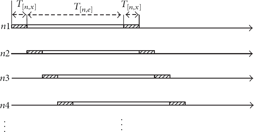
Timeline of cooperative processing.

3.2. Processing Validation

Consideration of the minimum execution time given the network bandwidth is needed before planning to build a distributed wireless sensor network application. As we mentioned, typically wireless sensor networks are operated under low bandwidth, which affects the total execution time (T). We use this minimum execution time ( $T_{\min }$ ) for the validation of distributed processing. If the minimum execution time is greater than the execution time ( $T_1$ ) on a single node, the distributed processing is valid.

It is impossible that T is less than propagation time for the whole data including data scattering and gathering. Therefore, distributed processing takes more time than processing on a single node if $T_1$ is less than $T_{\min }$ . We define the equation for validation as follows:

$$\begin{array}{cc}& T_{\mathrm{1}}>T_{\min }=\frac{\mathrm{2}L}{B},\end{array}$$

(3)

where L is the size of all data on the root node and B is the network bandwidth.

3.3. Total Execution Time

The total execution time can be calculated for two different cases according to two time points: point $P_A$ , when a task is completed by the first node, and point $P_B$ , when data distribution is completed, as shown in Figures 3 and 4.

Figure 3

Timeline when $P_A>P_B$ .

Figure 4

Timeline when $P_A<P_B$ .

Figure 3 shows the first case with 4 processing nodes, in which $P_A$ is greater than $P_B$ . The total execution time with n processing nodes ( $T_n$ ) is the sum of the time taken to reach $P_A$ and the completion time data transmission returning to the root node from $P_A$ .

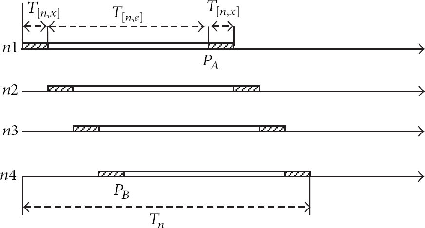
The second case is presented by Figure 4, which is when $P_A<P_B$ . In this case, the total execution time is the sum of the time taken to distribute data and return data from all nodes to the root node. The total execution time is not affected by the execution time ( $T_{[n,e]}$ ) on the processing node because $T_{[n,e]}$ is sufficiently short to not affect the total execution time.

$P_A$ is the sum of propagation time ( $T_{[n,x]}$ ) for chunk data and $T_{[n,e]}$ , and $P_B$ is $T_{[n,x]}$ times n. From these, the criterion that identifies the two cases mentioned above was obtained as follows:

$$\begin{array}{cc}& P_A-P_B=T_{\left[n,x\right]}\left(\mathrm{1}-n\right)+T_{\left[n,e\right]}.\end{array}$$

(4)

Therefore, the total execution time ( $T_n$ ) with n processing nodes can be calculated as follows:

$$\begin{array}{c}{T}_n=\{\begin{array}{cc}{T}_{\left[n,x\right]}\left(n+\mathrm{1}\right)+T_{\left[n,e\right]},\hfill & \text{if}\mathrm{\hspace{0.17em}\hspace{0.17em}}{T}_{\left[n,x\right]}\left(n-\mathrm{1}\right)<\mathrm{\hspace{0.17em}\hspace{0.17em}}{T}_{\left[n,e\right]}\hfill \\ \mathrm{2}n{T}_{[n,x]},\hfill & \text{otherwise}.\hfill \end{array}\mathrm{\hspace{0.17em}\hspace{0.17em}}\hspace{1em}\end{array}$$

(5)

3.4. Optimal Number of Processing Nodes

We measured the execution time when adding processing nodes. From Figure 5, the distributed processing performance does not improve with the addition of processing nodes. The inclusion of additional sensor nodes to processing leads to the wastage of network resources. We define the optimal number of processing nodes as the point at which an increase in the number of nodes does not decrease the total execution time.

Figure 5

Measured execution time.

When $T_{[n,x]}(\mathrm{1}-n)>T_{[n,e]}$ in (5), $T_n$ is equivalent to the total time required to send and receive data. This transmission time is not affected by the number of processing nodes and is only affected by data size and bandwidth, which means that the total execution time does not decrease once n satisfies the above condition. The optimal number of processing nodes is defined as

$$\begin{array}{cc}& n>\frac{T_{\left[n,e\right]}}{T_{\left[n,x\right]}}\mathrm{\hspace{0.17em}\hspace{0.17em}}+\mathrm{1}.\end{array}$$

(6)

$T_{[n,e]}$ and $T_{[n,x]}$ depend on the number of nodes. We add the following terms to (6) to eliminate this dependency:

$$\begin{array}{cc}& T_{\left[n,x\right]}=\frac{L_n}{B},\\ T_{[n,e]}=\frac{T_{\mathrm{1}}}{n},\end{array}$$

(7)

where, $T_1$ : time taken by a node for data processing, L: total data size, $L_n$ : split data size for n nodes ( $L/n$ ), and B: network bandwidth.

Consequently, the optimal number of processing nodes can be estimated as

$$\begin{array}{cc}& n>\frac{B{T}_{\mathrm{1}}}{L\mathrm{\hspace{0.17em}\hspace{0.17em}}}+\mathrm{1}.\end{array}$$

(8)

3.5. Implementation Issues

To apply the proposed execution estimation model to design a software system for a wireless sensor network, the following issues should be considered.

3.5.1. Premeasuring $T_1$ and B

The proposed method is based on data transmission time $T_{[n,x]}$ and execution time $T_1$ on a single node. These values are dependent on the data size and network bandwidth. If the data size is fixed, it can be assumed that $T_1$ is also a fixed value and has been measured before. The network bandwidth is specified by the network type, such as IEEE 802.15.4. However, the real network bandwidth necessary to send data varies with the specification according to packet size or protocol, so we suggest measuring the transmission rate in real time.

3.5.2. $T_{[n,e]}$ Estimation

In (7), we assume that $T_{[n,e]}$ quals $T_1/n$ . This means that $T_{[n,e]}$ is proportional to n. Nevertheless, the relationship between $T_1$ and $T_{[n,e]}$ can vary according to the task.

4. Experimental Environment

We measured transmission rates with the same packet size and protocol before evaluating the accuracy of our proposed model. Then, we calculated the total execution time and the optimal cluster size with the measured transmission rate and the data size. We compared the calculated results and the measured data via experiments. The experiments were conducted with TinyOS 2.x and a MICAz mote of UC Berkeley [10, 11].

4.1. Transmission Rates

The transmission rates are needed for our proposed equations. We measured the transmission time for the various data sizes. Figure 6 presents the sequence by which the application sends data and how to measure the transmission time. TinyOS is an event-driven operating system. When the application tries to send data, the scheduler returns the status immediately and signals the SendDone events after finishing transmission. Our implementation sends data in the SendDone event handler in divided packets repeatedly.

Figure 6

Sequence for measuring transmission rates.

The base station sets the timestamp after sending a command to the node implemented for the transmission task. Then, the base station calculates transmission rates after receiving all packets.

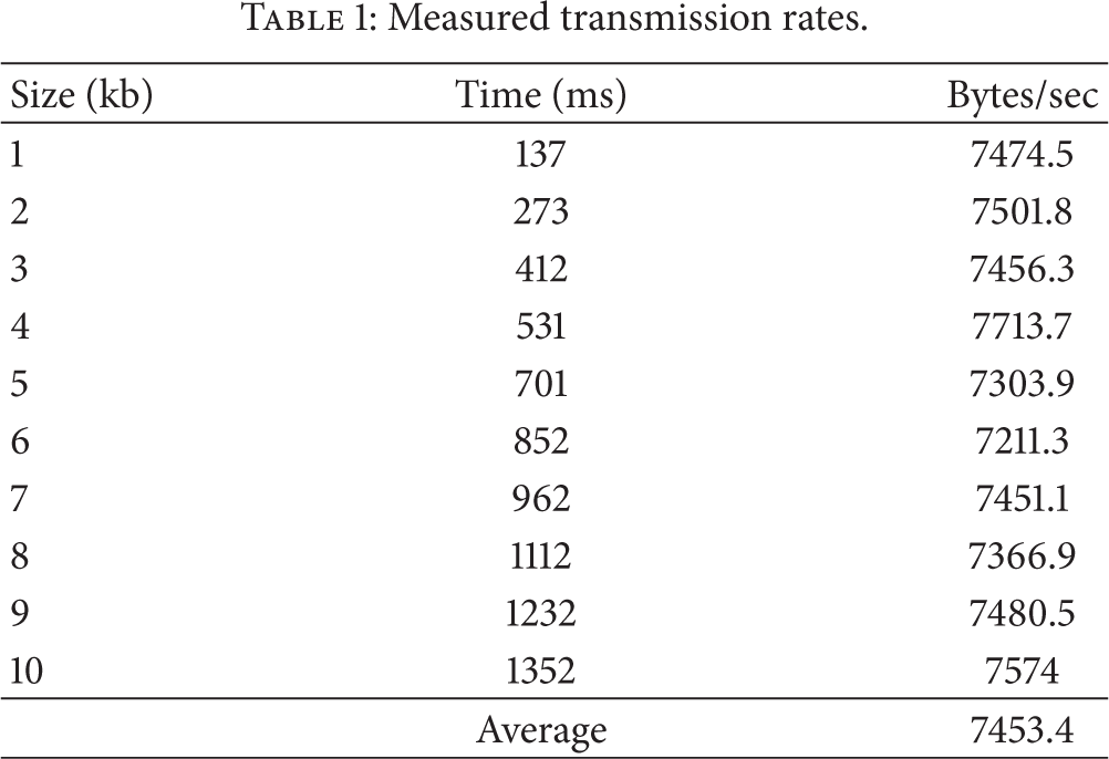
The measured transmission rates are presented in Table 1. In our other experiments, we used the measured average value of transmission rates as the network bandwidth.

Table 1

Measured transmission rates.

Size (kb)	Time (ms)	Bytes/sec
1	137	7474.5
2	273	7501.8
3	412	7456.3
4	531	7713.7
5	701	7303.9
6	852	7211.3
7	962	7451.1
8	1112	7366.9
9	1232	7480.5
10	1352	7574
	Average	7453.4

4.2. Validation

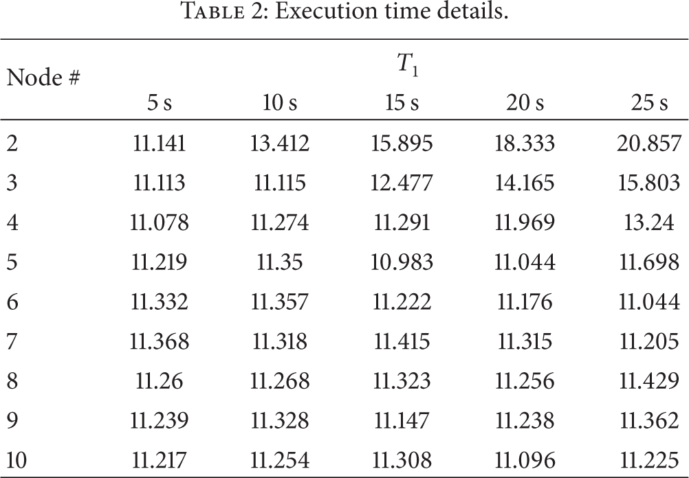
We propose a validation method to identify whether the total execution time of the distributed processing is shorter than that for processing on a single node. System designers could use the proposed method to check distributed performance with their own parameters. This experiment was conducted with a fixed data size ( $L=40$  kB) and a varying $T_1$ and number of nodes.

Figure 7 shows the measured execution time, and the details are presented in Table 2. Some results were even worse than $T_1$ because of the transmission time. From the table, a gain in execution time was not found when $T_1$ is 5 seconds and 10 seconds. The performance of the 5-second case was twice as bad as that for single node processing. In the case of 15 seconds, the execution time was approximately 16 seconds with 2 nodes but under the $T_1$ after 3 nodes. The cases of 20 seconds and 25 seconds showed a similar pattern to that of the case of 15 seconds.

Table 2

Execution time details.

Node #	$T_{\mathit{1}}$
	5 s	10 s	15 s	20 s	25 s
2	11.141	13.412	15.895	18.333	20.857
3	11.113	11.115	12.477	14.165	15.803
4	11.078	11.274	11.291	11.969	13.24
5	11.219	11.35	10.983	11.044	11.698
6	11.332	11.357	11.222	11.176	11.044
7	11.368	11.318	11.415	11.315	11.205
8	11.26	11.268	11.323	11.256	11.429
9	11.239	11.328	11.147	11.238	11.362
10	11.217	11.254	11.308	11.096	11.225

Figure 7

Execution time with fixed data size.

$T_{\min }$ is 10.99 seconds according to (3) and the measured transmission rates in the previous chapter. As we discussed in Section 3.4, no continuous processing performance improvement was found by the addition of processing nodes. Consequently, we were able to obtain conclusions that the execution time could not be shorter than $T_{\min }$ in any case and whether there would be a gain in execution time or not can be investigated as previously shown.

4.3. The Optimal Number of Processing Nodes

The optimal number of processing nodes was defined as the point after which there was no performance improvement in execution time. Figures 8 and 9 represent the measured total execution time and optimal number of nodes for each case. The optimal point is calculated via our proposed model.

Figure 8

Measured $T_n$ and number of optimal nodes ( $T_1=30$  s).

Figure 9

Measured $T_n$ and number of optimal nodes ( $L=50$  kB).

The first experiment was conducted with fixed $T_1$ as 30 s and various numbers of nodes and data sizes. The figure shows the optimal points plotted at a reasonable number of processing nodes for each case. In other words, performance improvements in time were not found after the optimal point. Figure 9 also shows that the optimal points are acceptable, which was conducted under the fixed data size and the various numbers of nodes and $T_1$ .

4.4. Execution Time Estimation

We measured the total execution time by varying the number of processing nodes. Figure 10 shows the measurements and the calculated $T_n$ based on the proposed model. The average error was found to be as small as 0.36 seconds.

Figure 10

Measured and estimated execution time ( $L=50$  kB, $T_1=50$  s).

No other tasks were included in the experiments, so the results have negligible error. For practical applications, the network status and other tasks should be considered.

5. Case Study: 2D FFT

The fast Fourier transform (FFT) is widely utilized for signal processing applications such as structural health monitoring and multimedia processing. We implemented a distributed 2D-FFT application and evaluated our model for this application. Data sizes of $64\times 64$ and $128\times 128$ and 2, 4, 8, 16, and 32 processing nodes were used. The root node distributes data and then the processing nodes execute a 1D-FFT. After returning all data, the root node transposes the matrix and repeats scattering and gathering.

As we discussed in Section 3.5, $T_1$ , the data transmission rates, and the relationship between $T_1$ and $T_{[n,e]}$ should be investigated in our model. We used the same data transmission rates as in Section 4. $T_1$ was measured from a single node implementation. A 2D-FFT with an $m\times n$ matrix is composed of an n m-point FFT, a transpose, and another m n-point FFT. We defined the unit of the task as an m-point FFT. Therefore, the relationship between $T_1$ and $T_{[n,e]}$ satisfies “ $T_{[n,e]}=T_1/n$ .”

The total execution time for a $64\times 64$ matrix was approximately 13 seconds on a single node. We measured the total execution time, varying the number of processing nodes from 2 to 32 for the same data. Figure 11 shows the measured and estimated total execution time for $64\times 64$ data. The execution time for transposing was ignored. $T_n$ was doubled because the number of rows and columns is identical, and the scattering and gathering were performed twice.

Figure 11

Total execution time for $64\times 64$ data.

In this case, the optimal number of processing nodes is estimated to be 13 via (8), and $T_{\min }$ is 1.92 seconds via (3). The optimal number of nodes, however, could be regarded as 16 nodes because the number of nodes in this application increases in two square steps. This means that the total execution time would not decrease if the number of nodes exceeded the optimal number of nodes.

From the results, the average error was found to be 1.2 seconds, and the trends in the total execution time bear a strong resemblance. At 16 processing nodes, the total execution time was the minimum for both the measured and estimated cases.

Figure 12 presents the results for a $128\times 128$ matrix. The average error was 2.9 seconds, and the optimal number of nodes is 16. At times, the uncertainty increased because of the significantly larger data size, which increased the average error.

Figure 12

Total execution time for $128\times 128$ data.

6. Conclusions

Wireless sensor networks provide an environment for distributed processing. The limited resources of the sensor nodes create a difficulty in designing a distributed system. For this reason, we have studied a distributed processing model in wireless sensor networks.

In this paper, we proposed a distributed processing model in wireless sensor networks. The methods to estimate the total execution time, validate distributed processing in terms of the execution time, and calculate the optimal number of processing nodes for distributed processing in wireless sensor networks were described.

We demonstrated the accuracy of the proposed model through experiments. First, the transmission rate was measured and was then used for the other experiments. Next, validation in terms of time was demonstrated. Through the validation equation, a system designer can decide whether distributed processing is needed or not. The experiments to confirm the optimal number of nodes were carried out with various options. The estimated optimal numbers of nodes were indicated with high accuracy. In the experiments for execution time estimation, the average error of the model was found to be as small as 0.36 seconds.

We implemented a 2D-FFT application and demonstrated that our model can be used for the application in the case study. The experiments had more errors than previous experiments because the proposed model does not consider other tasks on the node, and the real transmission rates are not identical all the time.

In our future research, the cost analysis in time and energy between centralized system and our proposed cooperative processing model will be performed. Furthermore, we will study the distributed processing model for multihop clusters and perform more experiments for other applications to improve the model.