Sage Journals: Discover world-class research

Abstract

Node deployment is one of the fundamental tasks for underwater acoustic sensor networks (UASNs) where the deployment strategy supports many fundamental network services, such as network topology control, routing, and boundary detection. Due to the complex deployment environment in three-dimensional (3D) space and unique characteristics of underwater acoustic channel, many factors need to be considered specifically during the deployment of UASNs. Thus, deployment issues in UASNs are significantly different from those of wireless sensor networks (WSNs). Node deployment for UASNs is an attractive research topic upon which a large number of algorithms have been proposed recently. This paper seeks to provide an overview of the most recent advances of deployment algorithms in UASNs while pointing out the open issues. In this paper, the deployment algorithms are classified into three categories based on the mobility of sensor nodes, namely, (I) static deployment, (II) self-adjustment deployment, and (III) movement-assisted deployment. The differences of the representative algorithms in aspects of sensor node types, computation complexity, energy consumption, deployment objectives, and so forth, are discussed and investigated in detail.

1. Introduction

Recently, advances in wireless sensor networks (WSNs) have motivated the development of underwater acoustic sensor networks (UASNs), which have become a compelling technology to enable and enhance applications such as environment monitoring, resource exploration, disaster prevention, pollution detection, and military surveillance [1].

UASNs are composed of different kinds of sensor nodes (i.e., surface sink, underwater sensor nodes, etc.) to collaboratively perform monitoring tasks over a three-dimensional (3D) space. A three-dimensional UASN architecture is shown in Figure 1. UASNs consist of static sensor nodes which are deployed both on the water surface and underwater and automatic mobile sensor nodes to perform collaborative monitoring tasks over a given monitored space. Static sensor nodes usually consist of a sensing device, a microcontroller, and an acoustic transceiver with a limited amount of energy. Automatic mobile sensor nodes such as autonomous underwater vehicles (AUVs), unmanned underwater vehicles (UUVs), and low-power gliders typically have plenty of energy which can be supplemented when needed. According to the application requirements, different kinds of sensor nodes can be deployed in UASNs, that is, surface sinks, underwater nodes, bottom nodes, and automatic mobile nodes. Surface sinks are responsible for data collection and global position system (GPS) signal acquisition; surface sinks can be either stationary or mobile. Underwater nodes are equipped with floating buoys which can be inflated by pumps to adjust their depths to cover the entire monitored space. Usually, bottom nodes are anchored at the bottom of the ocean to monitor the two-dimensional (2D) area or collaborate with underwater nodes and automatic mobile nodes to fulfill monitoring tasks in 3D space. Automatic mobile nodes can receive GPS signals while floating on the ocean surface, and then dive to a fixed depth and move among underwater nodes following a predefined trajectory to help with localization or information gathering, and so forth. Events are detected by sensor nodes locally and information is transferred to surface sinks by multihops or automatic mobile nodes using acoustic communication. Then, the data can be forwarded to onshore control centers which have larger storage capacity for future processing [2, 3].

Figure 1

A three-dimensional UASN architecture.

In UASNs, sensor nodes communicate with each other via acoustic signals, while due to the unique characteristics of underwater acoustic channels (large propagation delay, high error rate, multipath effects, etc. [4]), new algorithms and protocols should be specifically designed for 3D UASNs. Besides, UASNs normally operate in uncertain and mobile environments where free-floating underwater sensor nodes drift slowly with the water current. As a result, the relative motion of the transmitter or receiver may create the Doppler effect. Moreover, UASNs are energy-limited. Energy supplement is difficult because it requires underwater vehicles which are costly to operate. In summary, node deployment algorithms designed for UASNs need to address the adverse physical channel conditions and water mobility while staying energy-efficient [5]. Generally, the deployment strategies support many fundamental network services, such as network topology control, routing, and boundary detection, which will further influence the network performance. Therefore, node deployment is one of the fundamental tasks in UASNs.

In this paper, we give an overview of the state of the art related to deployment algorithms in UASNs and categorize them into static deployment, self-adjustment deployment, and movement-assisted deployment. The differences of the representative algorithms in aspects of sensor node types, computation complexity, energy consumption, deployment objectives, and so forth, are discussed. Furthermore, the characteristics of deployment algorithms in three categories are investigated and compared in detail.

The remainder of this paper is organized as follows. Section 2 discusses design considerations, classification, and evaluation criteria of deployment algorithms in UASNs. Section 3 presents a detailed analysis of recent deployment algorithms in three categories, respectively, and summarizes the algorithms. Section 4 makes a conclusion and discusses future research issues of deployment algorithms in UASNs.

2. Design Considerations and Classification of Deployment Algorithms

2.1. Design Considerations for UASNs

Notice that most existing algorithms and protocols in WSNs are aiming at 2D sensor networks. For example, Capone et al. considered a heterogeneous network scenario and presented an optimal framework based on integer linear programming to locate wireless gateways [6]. Y.-R. Tsai and Y.-J. Tsai proposed a step-by-step node deployment algorithm aimed at minimizing location estimation of the entire large-scale WSNs [7]. Wang et al. transformed traffic-aware relay node deployment problem into a Euclidean Steiner Minimum Tree (ESMT) problem and proposed a hybrid algorithm to maximize lifetime for data collection [8]. Guerriero et al. mathematically proposed and defined different optimization deployment models to achieve high performance in terms of energy consumption and travelled distance [9]. However, these algorithms may no longer be effective in UASNs. Because three-dimensional networks require additional design and computation complexity, many problems cannot be solved by extension of two-dimensional algorithms. Besides, the design of 3D algorithms is more difficult than that of 2D. Thus, new algorithms should be specifically designed for 3D UASNs by exploring rich geometric properties of 3D UASNs. UASNs are different from WSNs in many ways [1, 3, 9].

High Latency. GPS signal cannot propagate through water and radio frequency (RF) signal can be absorbed by water. Propagation delay of underwater acoustic signal is five orders of magnitude higher than in RF terrestrial channels.

Limited Bandwidth and High Transmission Loss. Underwater acoustic channel has characteristics of a limited bandwidth and multipath fading, which result in high bit error rates.

Node Mobility. Positions of underwater sensor nodes are easily affected by water current or fish swarm.

Limited Energy. Battery power is limited and difficult to be recharged without utilizing solar energy. Besides, more complex signal processing consumes more energy.

High Cost. Underwater sensor nodes are easier to fail because of fouling and corrosion, so they need extra protective shell.

Sparse and 3D Deployment. Monitoring an ocean column requires a 3D deployment. The costly underwater sensor nodes make it more likely to be a sparse deployment.

Thus, the deployment of UASNs is deemed to be sparser than that of WSNs and more difficult to guarantee the network performance. In face of these characteristics, new algorithms and protocols for 3D UASNs should be specifically designed to achieve the optimal deployment of each sensor.

Many researchers are currently engaged in designing deployment algorithms for UASNs. Due to the wide range of applications of UASNs and variety of underwater environment, different objective-oriented deployment algorithms could be designed to meet certain requirements. Typically, there are two types of architectures in UASNs, namely, (I) 2D UASNs for underwater bottom or surface monitoring and (II) 3D UASNs for underwater column monitoring [10]. In 2D UASNs, sensor nodes are anchored at the bottom of the ocean or floating on the ocean surface. In 3D UASNs, depths of sensor nodes can be adjusted by means of techniques.

2.2. Classification Based on Sensor Nodes' Mobility

There have been a large number of researches focusing on deployment issues in UASNs over the last few years. According to the mobility of sensors, the deployment algorithms can be classified into three categories, namely, static deployment, self-adjustment deployment, and movement-assisted deployment as shown in Figure 2. (I) Static deployment: all the sensors are static after initial deployment. Sensors are attached to surface buoys or anchored at the bottom of the ocean and they are assumed to have fixed positions. Static deployment is further classified into random deployment and regular deployment. (II) Self-adjustment deployment: underwater sensor nodes can adjust their depths by inflating floating buoys automatically or be driven to some desirable positions by mobile sensor nodes after initial deployment to meet certain requirements. Self-adjustment deployment is further classified into uniform coverage deployment and nonuniform deployment. (III) Movement-assisted deployment: there are underwater mobile sensor nodes patrolling over the monitored region to cooperate with other sensors to fulfill monitoring tasks. Some of the self-adjustment deployment algorithms and movement-assisted algorithms take sensor nodes' mobility into consideration, which is caused by water current or other marine animals.

Figure 2

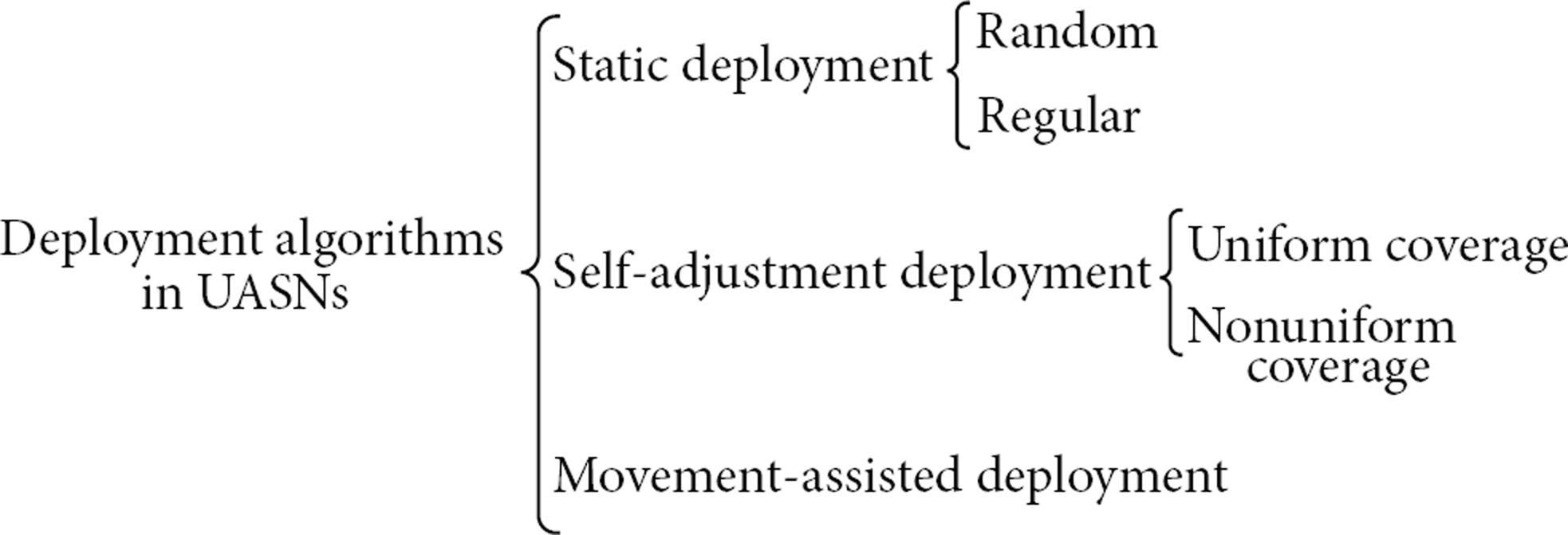
Classification of deployment algorithms for UASNs.

2.3. Evaluation Criteria

We summarize typical deployment algorithms of each category in the following aspects.

Sensor Node Types. Typically, there are at least two kinds of sensors in UASNs, namely, sink node and underwater sensor nodes. Some researchers define other kinds of sensor node, such as surface gateway, AUV, and mobile data collector, according to their deployment algorithms.

Distributed or Centralized. Generally speaking, the distributed algorithms are more suitable for UASNs, due to their scalability and computational efficiency. The centralized algorithms are easier to implement, but may suffer from network attack which will result in network failure.

Computation Complexity. The computation complexity of an algorithm is of vital importance since it directly influences the execution time of the algorithm. Besides, the computation complexity also has an impact on energy consumption.

Energy Consumption. The total energy consumption of a network is determined by summing up energy consumption of all the sensor nodes in the network. Due to the limited energy resource, the algorithm should be energy efficient.

Deployment Objectives. Since sensor network is a kind of application-oriented network, deployment algorithms with different objectives could be designed to meet certain requirements.

Main Advantages. Although different deployment algorithms have their own characteristics, each algorithm has its own advantages.

3. Analysis of Deployment Algorithms

3.1. Static Deployment

For simplicity, many deployment algorithms assume that sensors are static after initial deployment in UASNs, with the consideration of practical reasons such as deployment cost and algorithm complexity. For 2D UASNs, sensors are usually deployed only on the water surface or at the bottom of the monitored region. Bottom sensors may be organized in a cluster-based architecture and forward collected data to surface sinks by multihop paths. For 3D UASNs, sensors are floating in different depths to observe the entire monitored region. In both architectures, sensors do not actively change their positions after initial deployment.

3.1.1. Random

Random deployment is the most practical way in deploying sensors. If no prior knowledge of the to-be-monitored region is available or deterministic deployment of sensors is very risky or infeasible, random deployment often becomes the only option. Usually, random deployment serves as an initial phase of self-adjustment and movement-assisted deployment strategies. Senouci et al. categorized random placement strategies into simple and compound [11]. Simple strategies are mere variants of the simple diffusion strategy, whereas compound strategies are realized by repeated simple diffusion. Through simulations, they give design guidelines in using stochastic deployment strategies.

3.1.2. Regular

The main characteristic of regular deployment is that sensors are anchored at the vertex of polygons or polyhedrons.

Pompili et al. provided a mathematical deployment analysis for both two-dimensional and three-dimensional architectures [12]. For two-dimensional architecture, they proposed a triangular-grid deployment algorithm to use the minimum number of sensors to achieve both optimal sensing and communication coverage. In triangular-grid deployment, sensors are deployed at the vertex of equilateral triangles. They mathematically proved that overlapping areas of neighboring sensors can be minimized and the coverage ratio is equal to 1, when length of equilateral triangle d is $\sqrt{3}$ times of sensing range r, as shown in Figure 3. There is a trade-off between the number of sensors and achievable sensing coverage. The authors studied the dynamics of a sinking object and evaluated the trajectory of a sinking object under the impact of water current, which can be used to estimate the final position of a sinking object.

Figure 3

Triangular-grid deployment: (a) grid structure and side margins and (b) uncovered area $(Δ A B C)$ .

Ibrahim et al. formulated the gateway optimal deployment issue as an integer linear programming (ILP) problem [13]. Later, they proposed a multiple surface-level gateways deployment algorithm based on heuristic approaches to enhance network performance [14]. They used greed algorithm and greed-interchange algorithm to select optimal gateway positions among $m \times m$ candidate locations which are mesh of points. The authors provided a multisink architecture and presented guidelines for deciding the number and positions of surface gateways in UASNs. However, it is a two-dimensional sensor deployment issue indeed.

Nazrul Alam and Haas aimed at finding a node deployment strategy with 100% sensing coverage of a 3D space, while minimizing the number of sensors needed [15]. In this paper, the authors defined a metric called volumetric quotient, which is the ratio of the volume of a polyhedron to the volume of its circumsphere. The higher the volumetric quotient, the smaller the number of nodes required for full 3D coverage. The paper gives a detailed analysis of several space-filling polyhedrons deployment, namely, cube deployment, hexagonal prism deployment, rhombic dodecahedron deployment, and truncated octahedron deployment as shown in Figure 4. Simulation results indicated that truncated octahedral cells result in the best strategy, and the higher the volumetric quotient is, the smaller the number of nodes that is needed to meet the coverage and connectivity requirements.

Figure 4

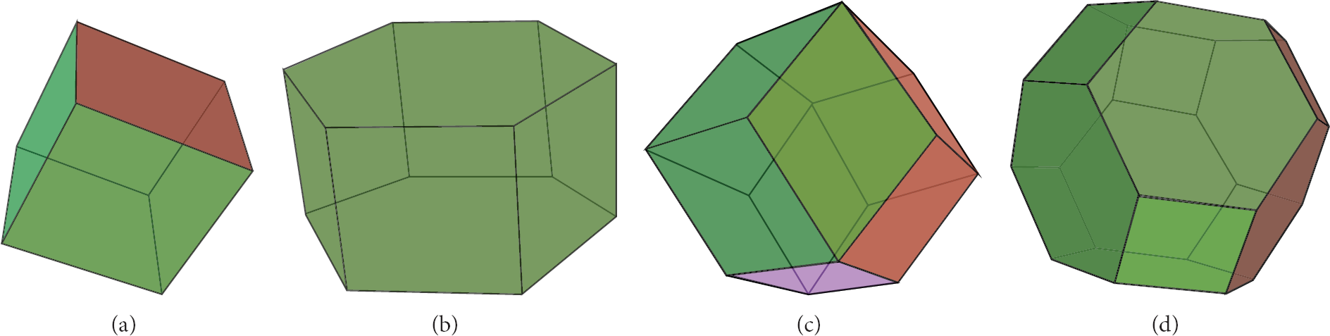
Several space-filling polyhedrons deployment: (a) cube deployment, (b) hexagonal prism deployment, (c) rhombic dodecahedron deployment, and (d) truncated octahedron deployment.

Felemban et al. formulated the optimal node placement as a nonlinear mathematical program with the objective of minimizing the transmission loss under a given monitored volume and number of sensor nodes [16]. Relay nodes are deployed next to each other in the 3D space forming tiled truncated octahedrons as presented in [15]. The main difference is that they considered the characteristics of underwater acoustic channels. Simulations showed that the operating frequency affects the number of nodes needed to cover a definite volume.

A UASN deployment algorithm (UDA) is proposed by Liu [17]. Different from [15, 16], UDA aims at determining and selecting the best cluster shape after partitioning the monitored region into layers and clusters. Clusters have shapes of cuboids, hexagonal prisms, rhombic dodecahedrons, and truncated octahedrons. Only the cluster-head in every cluster keeps alive for sensing and communicating. Once the cluster-head depletes its energy, a new cluster-head within the cluster will wake up and replace the old one. UDA sets different node densities at different layers to help prolonging lifetime of sensors close to sinks and balance the network energy consumption. However, there is no description about how to keep time synchronization when waking up a new cluster-head to maintain full connectivity and full coverage.

A multipath virtual sink architecture for UASNs is presented in [18] to overcome adverse link conditions. Virtual sinks are deployed at vertex of monitoring surface. The network dynamically selects shortest paths to deliver data over more routes to increase the probability of successful delivery instead of retransmissions. The algorithm ensures that data delivery continues to function even when a part of the network is temporarily nonoperational.

These static deployment algorithms enable easy and energy efficient deployment strategies for UASNs. They do not need auxiliary mobile sensor nodes to participate in deployment periodically. However, static deployment also suffers from some weaknesses. For instance, they cannot deal with real time event processing in large-scale UASNs.

3.2. Self-Adjustment Deployment

If the sensors have the ability of adjusting their positions in underwater environment after initial deployment to meet certain requirements, the corresponding algorithm is classified as the self-adjustment deployment. Each sensor is attached to a floating buoy. Sensor nodes can adjust their depths by controlling the length of the wires [19]. The depth adjustment system enables the underwater sensors to be deployed with a desired topology which can improve network connectivity and communication link over the whole monitored region. Moreover, relocated sensors at different depths based on a local agreement can efficiently reduce the coverage overlaps among the neighboring nodes.

3.2.1. Uniform Coverage

For three-dimensional architecture in [12], Pompili et al. proposed three deployment strategies, namely, 3D-random, bottom-random, and bottom-grid. Sensors are initially deployed at the bottom of the ocean. Then, each sensor is assigned to a target depth. Sensors float to the desired positions to achieve the target coverage ratio. However, they neglected to describe how to adjust sensor depths to maximize coverage ratio in a 3D space.

Akkaya and Newell proposed a distributed node deployment algorithm to reduce coverage overlaps based on the idea of graph coloring by using the relocation ability of underwater sensor nodes in a vertical direction [20]. At first, sensors are randomly deployed at the bottom of the ocean. The new locations in the vertical direction are computed by cluster headers based on the group IDs of the sensors. Then, sensors continue to adjust their depths by applying repelling forces to minimize coverage overlaps until there are no sensing overlaps for a node or a maximum number of rounds have arrived as depicted in Figure 5. The authors also assessed the performance of the proposed algorithm under a UASN water current mobility model and gave a detailed analysis of simulation results.

Figure 5

Distributed topology adjustment: (a) initialization, (b) clustering, (c) grouping, and (d) depth adjustment.

Xia et al. introduced a rigid theory and defined rigidity-coverage value as the evaluation criteria for the positions of underwater sensors [21]. They established a novel underwater self-organization deployment mechanism based on rigidity-driven mobile strategy. Sensors move randomly in the ocean until they meet their neighboring nodes. When a sensor node $s_{c}$ detects its neighboring node $s_{i}$ , $s_{c}$ and $s_{i}$ will assemble in a crowd. It is a distributed deployment algorithm. Sensors execute the rigidity-driven deployment process periodically without time synchronization. The simulations were carried out in the areas of 10 × 10 (2D) and 10 × 10 × 10 (3D) with the number of sensors varying from 10 to 15, respectively. Although they tested the performance of the deployment algorithm under the impact of water current, both the simulation area and the number of sensors are too small.

The mobility of underwater sensors makes the network topology slowly change and beinconveniently controlled. References [22, 23] aim at improving network coverage ratio and maintaining network connectivity when there are noncoverage areas or shadow zones. In [22], a dividing cube method is used to calculate the coverage ratio of an area. Then, two redeployment algorithms are proposed, of which one is based on the idea of adding new nodes, whereas the other is by the means of moving some redundant nodes from overcovered areas to noncoverage areas. Domingo presented an adaptive topology reorganization scheme to minimize the transmission loss and maintain network connectivity when a UASN is affected by shadow zones [23]. Sensor nodes are double units, operating as a single sensor, which are decoupled into two sensor nodes in the presence of a shadow zone. For instance, the sensor node $S_{i}$ is uncoupled into two sensor nodes $S_{i \to 1}$ and $S_{i \to 2}$ under the presence of a shadow zone as shown in Figure 6. $S_{i \to 1}$ and $S_{i \to 2}$ are connected to each other by a wire to maintain robust communication. In this way, connectivity between two neighbor nodes is maintained and latency as well as power consumption is reduced.

Figure 6

New scenario in the 3D UASN with a shadow zone.

3.2.2. Nonuniform Coverage

Since a UASN is a monitoring network, event detection is one of its main tasks. In nonuniform coverage deployment, how to adjust the positions of sensors according to the dynamic environment and targets to cover the event area in an optimal manner is a key issue in UASNs.

By simulating the behaviors of fish swarm and considering congestion control, a fish swarm-inspired sensor deployment (FSSD) algorithm was presented [24]. Sensors are nonuniformly deployed in the monitored region. FSSD algorithm enables sensors to cover the event area automatically by executing prey, follow, and swarm processes. FSSD algorithm seeks to make node distribution density match with event distribution density. They defined an evaluation criterion called event set coverage efficiency to evaluate the deployment performance. FSSD algorithm is a distributed algorithm with low computation complexity and high energy consumption.

The monitored area is divided into sectors with varying geographic size and acoustic characteristics [25]. Game Theory Field Design (GTFD) model is used to allocate sensors to sectors according to the visitation probabilities of an adversary. The authors compared GTFD model with Size-Aware Field Design (SAFD) model and Radius-Aware Field Design (RAFD) model. SAFD and RAFD only consider either the size of a sector or acoustic characteristics, respectively. Simulations showed that GTFD offers a significant improvement in terms of overall field detection capability against intelligent adversaries. But they did not explain how to deploy sensors in each sector. Besides, it is a centralized algorithm with 2D architecture and has high computation complexity.

Aitsaadi et al. addressed the issue of deploying a UASN in an area characterized by the geographical irregularity of the sensed event [26]. They proposed a geometric method called Differentiated Deployment Algorithm (DDA) based on a mesh representation method. By using a multiobjectives nonlinear optimization method, the optimal solution of DDA could be obtained. In DDA, authors considered triangles and rectangles during the hierarchical mesh. The basic idea is to permit progressive meshes division of a sensor field area as long as it is considered beneficial. New sensor nodes could be placed in equidistant locations to the vertices of the divided mesh. Or place an added node in the mid of one given arc of the mesh. It is a centralized algorithm, which is only applicable to static monitoring environment.

3.3. Movement-Assisted Deployment

In movement-assisted deployment, there exists AUVs, UUVs, low-power gliders, or other kinds of underwater mobile sensor nodes. They patrol over the monitored region under predefined trajectory to cooperate with other sensor nodes to fulfill monitoring tasks. Sensors can be attached to mobile sensor nodes as well and they can be driven to some desirable positions after initial deployment. Since underwater sensor nodes are fairly expensive and the costs quickly rise for deep water, underwater mobile sensor nodes can play more important roles compared with ordinary sensors in data collection, maximizing network coverage and real time event processing with limited hardware [27].

Teixeira et al. aimed at finding a control strategy that is able to drive a formation of AUVs from the initial to the target set of positions under the effect of external disturbances such as ocean current within a specified time [28]. They presented a leader-follower solution that relies on a simple uncertainty model to trigger surfacing events and two control strategies to position the agent within a certain distance of the target in the presence of disturbances.

Liu et al. and Ibrahim et al. studied the benefits of dynamic gateway redeployment [29, 30]. Both of the redeployment algorithms are triggered at fixed intervals. Liu et al. proposed a prediction assisted dynamic surface gateway placement (PADP) algorithm for mobile underwater sensor networks [29]. PADP applies a tracking scheme called interacting multiple model (IMM) to predict sensors positions, uses branch-and-cut method to solve optimization problem, and adopts a disjoint-set data structure to partition sensors into clusters. By using PADA, gateways are deployed based on both sensor nodes current and future positions of sensor nodes, so coverage is well maintained. Ibrahim et al. modeled surface gateway deployment problem as a graph optimization problem [30]. The problem is to choose a subset of the candidate surface gateway satisfying a set of flow conservation constraints. The main difference from the gateway deployment problem they addressed in [14] is that they considered a dynamic gateway deployment strategy to cope with changes and fine-tune deployments. They also integrated the gateway deployment optimization framework into Aqua-Sim, a NS2-based UASN simulator.

The idea of mobile data collectors has been proposed in the literature for UASNs [31, 32]. Data collectors patrol over the monitored region under predefined trajectory through an optimization process. When the network is not a real time processing application, data can be stored at sensors until a mobile data collector is in the vicinity. Alsalih et al. divided the lifetime of the network into fixed length rounds and found the optimal locations of data collectors together with multihop routing paths using integer linear program (ILP) solver at the beginning of each round. The delay tolerant placement and routing (DTPR) scheme and the delay constrained placement and routing (DCPR) scheme are proposed to deliver the generated data from all sensor nodes to data collectors. The DCPR scheme has a boundary on how much time a data unit may spend on its way to a data collector. The objective function takes into account both the current residual energy and future energy expenditure of each sensor node. Experimental results showed that both of the schemes have the potential to prolong the lifetime of a UASN significantly.

The deployment of AUVs to collect data from underwater sensor networks has drawn much attention recently [33, 34]. AUV must plan its trajectory to minimize travel distance and maximize information gathering. Hollinger et al. proposed methods for solving this problem by extending approximation algorithms of variants of traveling salesperson problem (TSP) as shown in Figure 7 [33]. Williams developed a new adaptive strategy for performing data collection with a sonar-equipped AUV by adapting AUV survey route, which is based on the environmental characteristics observed in the data itself [34].

Figure 7

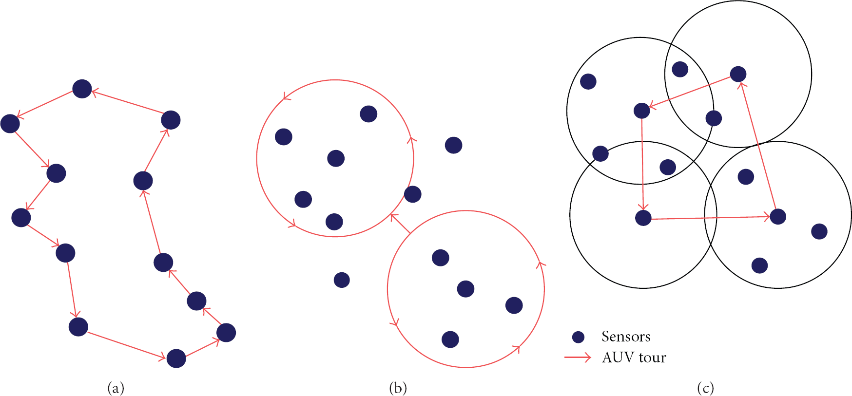
Example tours using different neighborhood types: (a) standard traveling salesperson tour, (b) tour circling a maximal independent set of neighborhoods, (c) tour visiting the center of a covering set of neighborhoods.

Yoon and Qiao focused on how to intelligently control multiple AUVs to complete the overall mission [35]. They proposed a cooperative rendezvous scheme called synchronization-based survey (SBS) to facilitate cooperation among several AUVs when surveying a large area. SBS has three variants, namely, alternating column synchronization (ACS), strict line synchronization (SLS), and x synchronization (XS). In SBS, AUVs form an intermittently connected network (ICN) in that they periodically meet each other for data aggregation, control signal dissemination, and AUV failure detection and recovery.

3.4. Summaries

In this section, we summaries the above-mentioned algorithms based on evaluation criteria presented in Section 2. From Table 1, we can conclude that each algorithm has its own advantages and no one is absolutely the best.

Table 1

Summary of the deployment algorithms.

Categories	Algorithms	Sensor types	Distributed or centralized	Computation complexity	Energy consumption	Deployment objectives	Main advantages
Static deployment	Ref. [12]	uw-sensor, UG	Centralized	Low	Low	Minimize overlapping coverage	Evaluate sinking objects' trajectory
	Ref. [14]	uw-sensor, UG	Distributed	High	Low	Gateway deployment optimization	Complexity analysis
	Ref. [15]	uw-sensor	Distributed	High	Low	Guarantee 100% coverage	Analysis of several space-filling polyhedrons
	Ref. [16]	uw-sensor, SG, RN	Centralized	High	Low	Minimize transmission loss	Detailed simulation analysis
	Ref. [17]	uw-sensor, CH	Centralized	High	Low	Maximize network lifetime	Clustering and duty-cycled network
	Ref. [18]	uw-sensor, virtual sink	Distributed	Low	Low	Ensure successful data delivery	Robustness

Self-adjustment deployment	Ref. [20]	uw-sensor, CH	Distributed	Low	High	Minimize overlapping coverage	Consider the influence of water current
	Ref. [21]	uw-sensor	Distributed	Low	High	Maximize coverage and connectivity	Consider the influence of water current
	Ref. [22]	uw-sensor	Centralized	Low	High	Minimize noncoverage areas	Coverage maintenance
	Ref. [23]	uw-sensor	Distributed	Low	Low	Maintain network connectivity	Energy-efficient
	Ref. [24]	uw-sensor	Distributed	Low	High	Cover the event areas automatically	Swarm intelligent algorithm
	Ref. [25]	uw-sensor	Centralized	High	Low	Allocates sensors follow event distribution	Event-driven-based nonuniform coverage
	Ref. [26]	uw-sensor	Centralized	High	Low	Achieve differentiated deployment	Differentiated coverage

Movement-assisted deployment	Ref. [28]	uw-sensor, AUV	Distributed	Low	High	Drive the AUV to target positions	Event-based
	Ref. [29]	uw-sensor, SG	Distributed	Low	High	Maximize coverage	Predict future positions
	Ref. [30]	uw-sensor, SG	Distributed	High	High	Minimize average end-to-end delay	Finding a near-optimal solution
	Ref. [31]	uw-sensor, DC	Distributed	High	High	Maximize network lifetime	Predict future energy expenditure
	Ref. [32]	uw-sensor, DC	Distributed	High	High	Maximize network lifetime	Delay constraints
	Ref. [33]	uw-sensor, AUV	Centralized	High	High	Minimize travel time	Consider different communication quality
	Ref. [34]	uw-sensor, AUV	Centralized	Low	High	Minimize travel time	Ensure the quality of collected data
	Ref. [35]	uw-sensor, AUV	Distributed	Low	High	Minimize travel time and distance	Failure detection and recovery

Uw-sensor: underwater sensor, UG: underwater gateway, SG: surface gateway, RN: relay node, CH: cluster head, SG: surface gateway, DC: data collector.

Generally speaking, most of the static deployment algorithms are centralized because sensor nodes are deployed uniformly at the beginning of the algorithms. Computation complexity and energy consumption is relatively low. A majority of static deployment algorithms aim at maximizing network coverage and minimizing sensor nodes that are needed in UASNs. However, the algorithms always neglect the mobility caused by water current which is inevitable in underwater environment.

In general, computational complexity and energy consumption of the self-adjustment deployment algorithms are larger than that of static deployment algorithms, because some of the sensor nodes can adjust their positions automatically to meet certain requirements. Due to unpredictable movement of sensor nodes in hybrid UASNs, some of the literature take sensor mobility into consideration by using a mobile model.

Since almost all the movement-assisted algorithms deploy mobile sensor nodes to help improving the network performance, the energy consumption of the movement-assisted algorithms is the largest among the three categories. Considering the costs and functions of mobile sensor nodes, fewer mobile sensor nodes are deployed in a UASN. Thus, the deployment problem is transformed into a path planning problem of mobile sensor. Most movement-assisted algorithms regard minimizing the total travel time and travel distance as one of their deployment objectives.

4. Conclusion and Future Research Issues

In this paper, we investigate the deployment issue in UASNs, which is a fundamental problem closely related to the quality of service of UASNs. We classify recent underwater deployment algorithms into three categories and give a comprehensive survey of them. Then, we summarize typical deployment algorithms in terms of sensor node types, computation complexity, energy consumption, and so forth, and make comparisons of three categories.

In recent years, many innovative solutions and ideas are used to design deployment algorithms in UASNs. The future research issues of deployment algorithms are possibly as follows. (i)

Since underwater sensor nodes inevitably move with water current, designing a mobility model is an important issue. When taking mobility into consideration, underwater deployment algorithms will become more effective.

(ii)

The existing deployment algorithms are mainly suitable to small-scale networks. However, many practical underwater monitored spaces are large-scale. Thus, deployment algorithms which are suitable for large-scale UASNs should be specifically designed.

(iii)

Since almost all the applications in UASNs are closely related to the locations of sensor nodes and the studying of node deployment also serves for localization, deployment algorithms and optimal path planning for mobile anchor nodes in large-scale UASNs should be specifically designed.

(iv)

A majority of the current deployment algorithms are based on a credible environment. However, in real applications, sensor nodes may be deployed in an unsafe and complex environment. Thus, failure node recovering algorithms or redundant node deployment algorithms are needed in order to avoid network partition.

(v)

To the best of our knowledge, few researches focus on the deployment of duty-cycled sensor nodes in UASNs to dynamically collaborate to prolong network lifetime. In duty-cycled environment, sensor nodes are allowed to be active or asleep periodically to reduce unnecessary energy consumption.

(vi)

Since underwater sensor nodes are fairly expensive and the costs quickly rise for deep water, sensor nodes must have different sensing and communication ranges in real applications. Thus, future researches should focus on designing deployment algorithms for heterogeneous UASNs.

(vii)

It is important to design systematic evaluation criteria to analyze the performance of different underwater deployment algorithms.

Footnotes

Acknowledgments

The work is supported by the Applied Basic Research Program of Changzhou Science and Technology Bureau, no. CJ20120028, the Scientific Research Foundation for the Returned Overseas Chinese Scholars, State Education Ministry, the Applied Basic Research Program of Nantong Science and Technology Bureau, no. BK2013032, and the Natural Science Foundation of Jiangsu Province of China, no. BK20131137.

References

Akyildiz

I. F.

Pompili

Melodia

Underwater acoustic sensor networks: research challenges

Ad Hoc Networks 2005 3 3 257 279

2-s2.0-13944252629

10.1016/j.adhoc.2005.01.004

Tan

H.-P.

Diamant

Seah

W. K. G.

Waldmeyer

A survey of techniques and challenges in underwater localization

Ocean Engineering 2011 38 14-15 1663 1676

2-s2.0-80052758366

10.1016/j.oceaneng.2011.07.017

Manjula

R. B.

Manvi

S. S.

Issues in underwater acoustic sensor networks

International Journal of Computer and Electrical Engineering 2011 3 1 1793 8163

Erol-Kantarci

Mouftah

H. T.

Oktug

Localization techniques for underwater acoustic sensor networks

IEEE Communications Magazine 2010 48 12 152 158

2-s2.0-78650880584

10.1109/MCOM.2010.5673086

Partan

Kurose

Levine

B. N.

A survey of practical issues in underwater networks

Proceedings of the 1st ACM International Workshop on Underwater Networks (WUWNet '06)

September 2006

ACM

17 24

2-s2.0-34247377791

10.1145/1161039.1161045

Capone

Cesana

Donno

D. D.

Filippini

Deploying multiple interconnected gateways in heterogeneous wireless sensor networks: an optimization approach

Computer Communications 2010 33 10 1151 1161

2-s2.0-77955266835

10.1016/j.comcom.2010.01.004

Tsai

Y.-R.

Tsai

Y.-J.

Sub-optimal step-by-step node deployment algorithm for user localization in wireless sensor networks

Proceedings of the IEEE International Conference on Sensor Networks, Ubiquitous, and Trustworthy Computing (SUTC '08)

June 2008

114 121

2-s2.0-50949100876

10.1109/SUTC.2008.33

Wang

Liu

Traffic-aware relay node deployment: maximizing lifetime for data collection wireless sensor networks

IEEE Transactions on Parallel and Distributed Systems 2011 22 8 1415 1423

2-s2.0-79959734488

10.1109/TPDS.2011.20

Guerriero

Violi

Natalizio

Loscri

Costanzo

Modelling and solving optimal placement problems in wireless sensor networks

Applied Mathematical Modelling 2011 35 1 230 241

2-s2.0-77955660758

10.1016/j.apm.2010.05.020

10.

Chen

Shen

Sun

The deployment algorithms in wireless sensor net works: a survey

Information Technology Journal 2009 8 3 293 301

2-s2.0-62749086433

10.3923/itj.2009.293.301

11.

Senouci

M. R.

Mellouk

Aissani

An analysis of intrinsic properties of stochastic node placement in sensor networks

Proceedings of the Global Communications Conference (GLOBECOM '12)

December 2012

494 499

12.

Pompili

Melodia

Akyildiz

I. F.

Three-dimensional and two-dimensional deployment analysis for underwater acoustic sensor networks

Ad Hoc Networks 2009 7 4 778 790

2-s2.0-58149178884

10.1016/j.adhoc.2008.07.010

13.

Ibrahim

Cui

J.-H.

Ammar

Surface-level gateway deployment for underwater sensor networks

Proceedings of the Military Communications Conference (MILCOM '07)

October 2007

1 7

2-s2.0-47949113744

10.1109/MILCOM.2007.4454996

14.

Ibrahim

Cui

J.-H.

Ammar

Efficient surface gateway deployment for underwater sensor networks

Proceedings of the 13th IEEE Symposium on Computers and Communications (ISCC '08)

July 2008

1177 1182

2-s2.0-55849151358

10.1109/ISCC.2008.4625609

15.

Nazrul Alam

S. M.

Haas

Z. J.

Coverage and connectivity in three-dimensional networks

Proceedings of the 12th Annual International Conference on Mobile Computing and Networking (MOBICOM '06)

September 2006

346 357

2-s2.0-33751061514

16.

Felemban

Shihada

Jamshaid

Optimal node placement in underwater wireless sensor networks

Proceedings of the Advanced Information Networking and Applications (AINA '13)

March 2013

492 499

17.

Liu

A deployment algorithm for underwater sensor networks in ocean environment

Journal of Circuits, Systems and Computers 2011 20 6 1051 1066

2-s2.0-80155153046

10.1142/S021812661100775X

18.

Seah

W. K. G.

Tan

H.-X.

Multipath virtual sink architecture for underwater sensor networks

Proceedings of the OCEANS—Asia Pacific

May 2007

1 6

2-s2.0-50249187546

10.1109/OCEANSAP.2006.4393933

19.

Pompili

Melodia

Akyildiz

I. F.

Deployment analysis in underwater acoustic wireless sensor networks

Proceedings of the 1st ACM International Workshop on Underwater Networks (WUWNet '06)

September 2006

48 55

2-s2.0-34247391564

10.1145/1161039.1161050

20.

Akkaya

Newell

Self-deployment of sensors for maximized coverage in underwater acoustic sensor networks

Computer Communications 2009 32 7–10 1233 1244

2-s2.0-65649114733

10.1016/j.comcom.2009.04.002

21.

Xia

Zheng

Rigidity driven underwater sensor self-organized deployment

Chinese Journal of Computers 2013 36 3

22.

Bin

Ren

Lin

Yang

Zeng

Wen

The redeployment issue in underwater sensor networks

Proceedings of the IEEE Global Telecommunications Conference (GLOBECOM '08)

December 2008

1 6

2-s2.0-67449091661

10.1109/GLOCOM.2008.ECP.978

23.

Domingo

M. C.

Optimal placement of wireless nodes in underwater wireless sensor networks with shadow zones

Proceedings of the 2nd IFIP Wireless Days (WD '09)

December 2009

1 6

2-s2.0-77952653786

10.1109/WD.2009.5449707

24.

Xia

Wang

C.-S.

Zheng

Jiang

J.-G.

Fish swarm inspired underwater sensor deployment

Acta Automatica Sinica 2012 38 2 295 302

2-s2.0-84858031852

10.3724/SP.J.1004.2012.00295

25.

Golen

E. F.

Mishra

Shenoy

An underwater sensor allocation scheme for a range dependent environment

Computer Networks 2010 54 3 404 415

2-s2.0-75949105882

10.1016/j.comnet.2009.09.016

26.

Aitsaadi

Achir

Boussetta

Pujolle

Differentiated underwater sensor network deployment

Proceedings of the OCEANS—Europe

June 2007

1 6

2-s2.0-36348967648

27.

Wang

Liu

Guo

Three-dimensional ocean sensor networks: a survey

Journal of Ocean University of China 2012 11 4 436 450

28.

Teixeira

P. V.

Dimarogonas

D. V.

Johansson

K. H.

Sousa

Event-based motion coordination of multiple underwater vehicles under disturbances

Proceedings of the IEEE Sydney OCEANS

May 2010

1 6

2-s2.0-78349244856

10.1109/OCEANSSYD.2010.5603980

29.

Liu

Han

Al-Bzoor

Zuba

Cui

J. H.

Ammar

R. A.

Rajasekaran

PADP:Prediction assisted dynamic surface gateway placement for mobile underwater networks

Proceedings of the IEEE Symposium on Computers and Communications (ISCC '12)

2012

139144

30.

Ibrahim

Liu

Al-Bzoor

Cui

J. H.

Ammar

Towards efficient dynamic surface gateway deployment for underwater network

Ad Hoc Networks 2013 11 8 2301 2312

31.

Alsalih

Hassanein

Akl

Placement of multiple mobile data collectors in underwater acoustic sensor networks

Wireless Communications and Mobile Computing 2008 8 8 1011 1022

2-s2.0-54949141185

10.1002/wcm.656

32.

Alsalih

Hassanein

Akl

Delay constrained placement of mobile data collectors in underwater acoustic sensor networks

Proceedings of the 33rd IEEE Conference on Local Computer Networks (LCN '08)

October 2008

91 97

2-s2.0-58049091487

10.1109/LCN.2008.4664156

33.

Hollinger

G. A.

Mitra

Sukhatme

G. S.

Autonomous data collection from underwater sensor networks using acoustic communication

Proceedings of the IEEE/RSJ International Conference on Intelligent Robots and Systems (IROS '11)

September 2011

3564 3570

2-s2.0-84455170077

10.1109/IROS.2011.6048662

34.

Williams

D. P.

AUV-enabled adaptive underwater surveying for optimal data collection

Intelligent Service Robotics 2012 5 1 33 54

2-s2.0-84855337229

10.1007/s11370-011-0102-y

35.

Yoon

Qiao

Cooperative search and survey using Autonomous Underwater Vehicles (AUVs)

IEEE Transactions on Parallel and Distributed Systems 2011 22 3 364 379

2-s2.0-79551538604

10.1109/TPDS.2010.88

A Survey on Deployment Algorithms in Underwater Acoustic Sensor Networks

Abstract

1. Introduction

2. Design Considerations and Classification of Deployment Algorithms

2.1. Design Considerations for UASNs

2.2. Classification Based on Sensor Nodes' Mobility

2.3. Evaluation Criteria

3. Analysis of Deployment Algorithms

3.1. Static Deployment

3.1.1. Random

3.1.2. Regular

3.2. Self-Adjustment Deployment

3.2.1. Uniform Coverage

3.2.2. Nonuniform Coverage

3.3. Movement-Assisted Deployment

3.4. Summaries

4. Conclusion and Future Research Issues

Footnotes

Acknowledgments

References