
Abstract
The dynamic modeling of a hub-tapered flexible beam system which is rotating in a plane is investigated. In the modeling, the high-order terms related with the nonlinear coupling term are retained, which are ignored in the first-order approximation coupling modeling. So, this model can also be called a high-order approximation coupling model, which cannot only be used in the case of small deformation but also in the case of large deformation. Solving for this mathematical model, we can obtain the dynamics of the system. Examples are given to indicate the differences between the high-order approximation coupling model and the first-order approximation coupling model. Also, the natural frequencies are studied through the transversal bending vibration analysis. The width ratio and the height ratio of the tapered beam are shown to have great influences on the transversal bending natural frequencies.
1. Introduction
Dynamics of the flexible structures can be affected by many factors, such as the shape and the motion. It is found that the dynamics of the flexible structure with large overall motion has an essential difference from the dynamics of that on an immobile base. In the past three decades, the dynamic modeling of a rotating flexible beam has received extensive research efforts [1–18]. Kane et al. [1] investigated a rotating flexible cantilever beam by using the traditional coupling model, which showed that this model fails to describe the dynamic behavior of the beam when it is at high rotation speed; and “Dynamic Stiffening” [1] was first pointed out. Then, many methodologies were developed to capture the dynamic stiffening term. Yoo and Shin [6] derived the motion equations of a rotating cantilever beam based on a new dynamic modeling method. The derived equations (governing stretching and bending motions) were all linear, so they could be directly used for the vibration analysis including the coupling effect, which could not be considered in the conventional modeling method. References [7–10] presented the first-order approximation coupling (FOAC) model, which is based on the theory of continuum medium mechanics and the theory of analysis dynamics. The FOAC model considered the second-order coupling term of longitudinal displacement caused by transversal deformation, while the traditional zeroth-order approximation coupling (ZOAC) model assumed small deformation in structural dynamics, where the longitudinal and transversal deformations are uncoupled. However, the FOAC model can only be used in the case of small deformation. Liu and Hong [11] presented a high-order approximation coupling (HOAC) model and showed that the HOAC model can be approximated to the FOAC model in the case of small deformation. However, the distinctions between HOAC model and FOAC model were not indicated.
Great progress has been made in the research on rotating flexible beam, but all the work mentioned above focused on the uniform beam. In some realistic engineering examples, such as turbine blades, the huge flagelliform antennas on the spacecraft, the cross sections of these structures are always variational along the length. We will get a more accurate dynamic analysis if we use the tapered beam model instead of the uniform beam model. Reference [14] investigated the free bending vibration of rotating tapered beams by using the dynamic stiffness method. The range of problems considered included beams for which the height and/or width of the cross section vary linearly along the length. A parametric study was carried out to demonstrate the effects of rotational speed, taper ratio, and hub radius on the natural frequencies and mode shapes of the tapered beams. Reference [15] investigated the intrinsic characteristics and the flexible motion of the tapered Euler-Bernoulli beam with tip mass and a rotating hub. Dynamic equations were derived from the extended Hamilton principle and the FOAC model. By comparing the uniform and the tapered system in the same condition, the obtained results indicated that a little difference in section can cause a significant difference in natural frequencies and dynamics response.
Since the FOAC model neglected some high-order terms in the dynamic equations, it could not be used in the large deformation problems [16]. So an exact dynamic model is needed to solve the large deformation problems. Shabana [17, 18] presented an absolute nodal coordinate method for the large rotation and deformation problems, and some examples were given to demonstrate the use of the absolute nodal coordinate formulation in the large rotation and deformation analysis of flexible bodies. The absolute nodal coordinate method can solve the large deformation problem of the flexible body very well. However, it cannot distinguishthe rigid body motion from the elastic deformation of the flexible body. Small deformation problems also should be treated as large deformation problems.
In this paper, we will study the dynamics of a hub-tapered beam system by using a high-order approximation coupling (HOAC) model, which cannot only be used in the small deformation problems but also large deformation problems. Both the transversal deformation and the longitudinal deformation of the flexible beam are considered. And in the total longitudinal deformation, the nonlinear coupling term, also known as the longitudinal shortening caused by transversal deformation, is considered. The assumed mode method (AMM) is used to describe the deformation of the flexible beam. The rigid-flexible coupling dynamic equations are established via employing the second kind of Lagrange's equation, retaining the high-order terms synchronously. Solving for this mathematical model, we can obtain the dynamics of the system.
2. Dynamic Equations
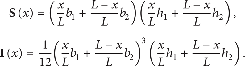
The system considered here is a flexible tapered beam driven by a hub rotor, as shown in Figure 1, which we call hub-beam system. The hub is assumed to be rigid with radius a and rotary inertia Joh. Applied at the hub, there is a torque τ. The flexible beam is a tapered Euler-Bernoulli beam (Figure 2) with length L and mass density ρ. The section area of the beam is S(x), and the section moment of inertia about
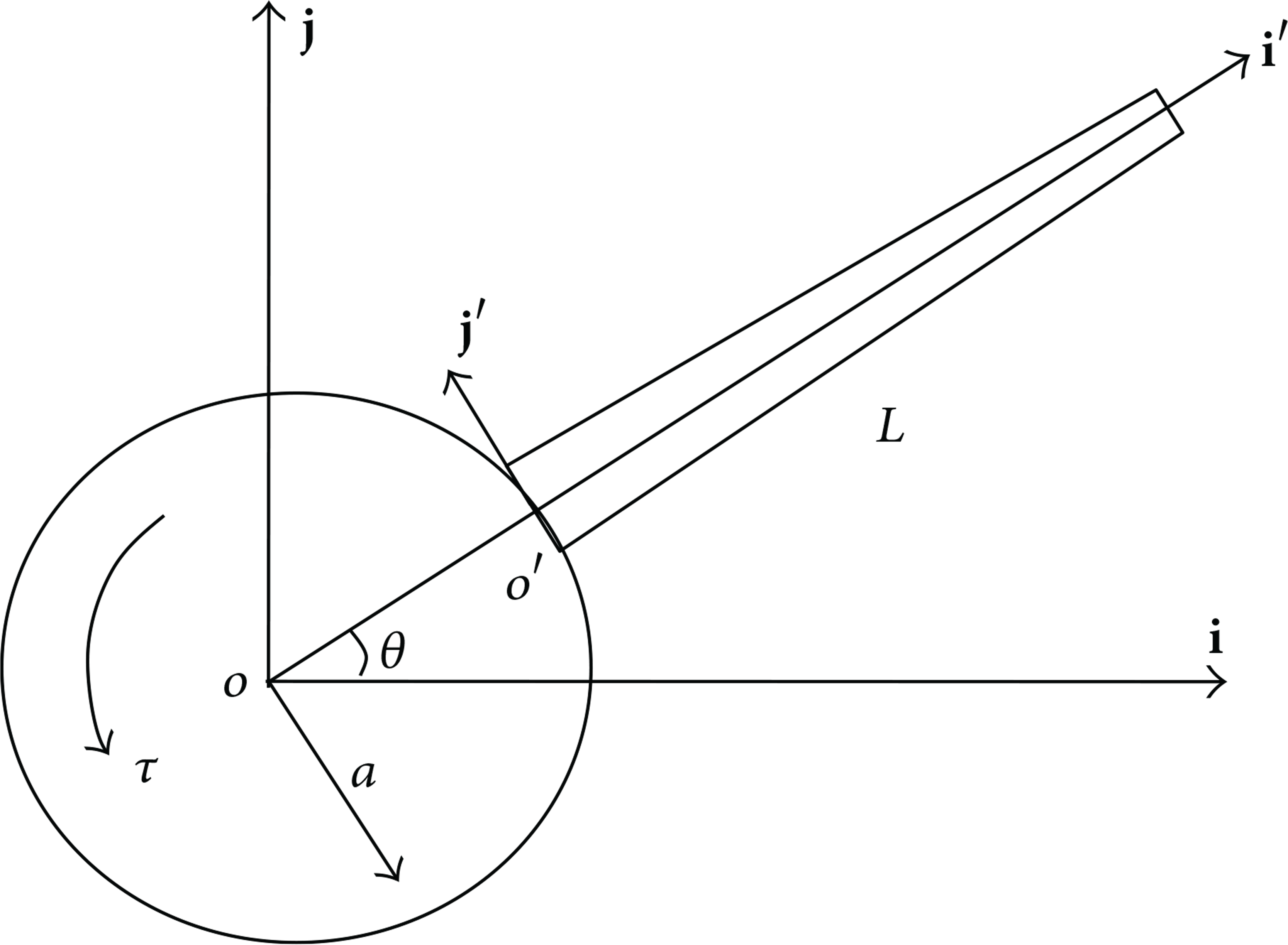
Schematic diagram of the system.
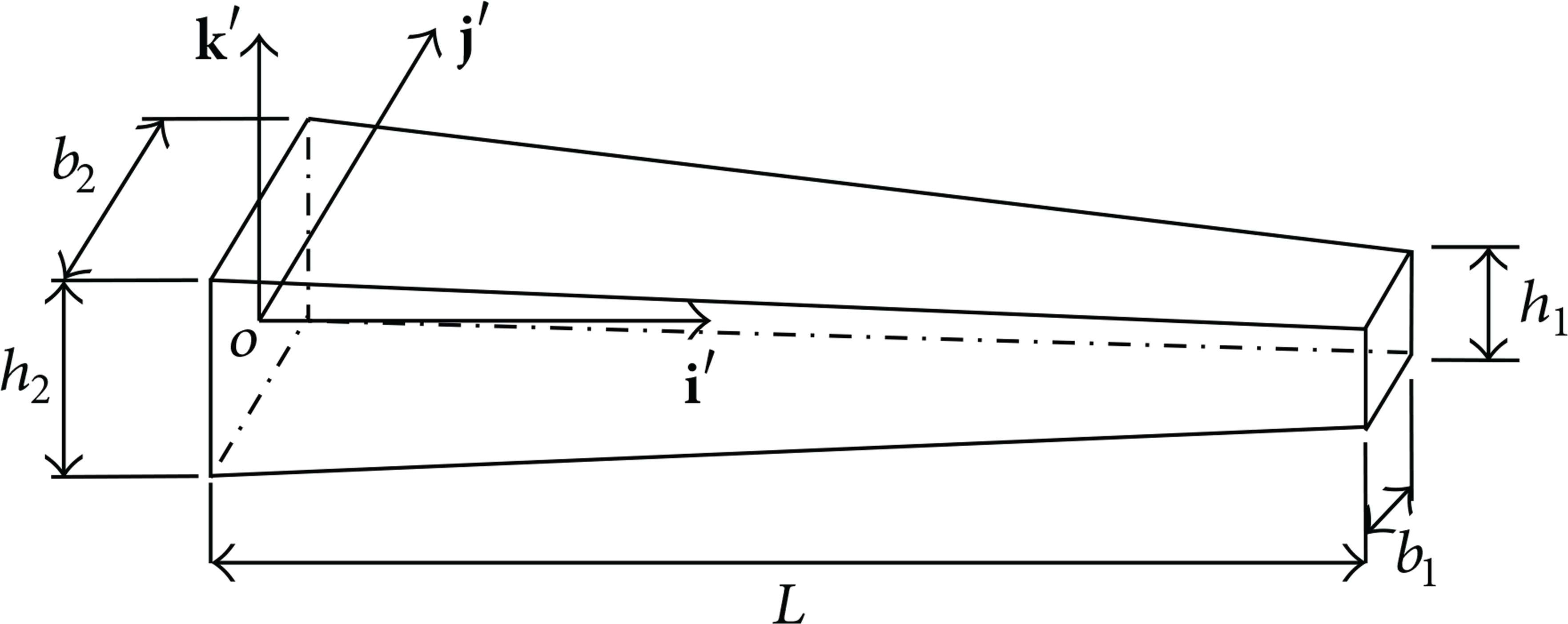
Schematic diagram of the tapered beam.
The coordinate systems used in developing the model are shown in Figure 3. Wherein o –

The deformation of the beam.
2.1. Kinetic Energy
To a generic point P(x) on the beam, the deformed position vector to point o can be expressed as

where w1(x, t) is the axial extension quantity, w2(x, t) is the transversal deformation, and w c (x, t) is the axial shorten caused by transversal deformation. w c (x, t) is also called the coupling deformation. In the ZOAC model, we usually used the small deformation assumption in structure dynamics but ignored the coupling deformation w c (x, t). When the large overall motion is at high speed, the coupling deformation w c (x, t) will have a significant influence on the dynamic characteristic of the system. w c (x, t) can be expressed as

The velocity vector of the point P(x) can be obtained by differentiating Equation (2) as follows:

then, the kinetic energy of the system can be expressed as
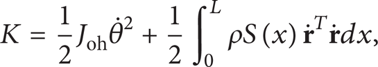
where the first part is the kinetic energy of the hub and the second part is the kinetic energy of the beam.
2.2. Potential Energy
As the beam is constrained in the horizontal plane, the gravitational potential energy can be ignored here. So, the potential energy of the system can be expressed as
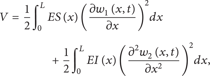
where the first part is the stretching energy of the beam and the second part is the bending energy of the beam.
2.3. Dynamic Equations
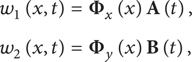
The assumed mode method (AMM) is used to describe the deformation of the flexible beam. The axial deformation w1(x, t) and the transversal deformation w2(x, t) can be expressed as
where Φ
x
(x)∊

where

Take the generalized coordinates

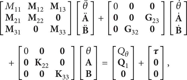
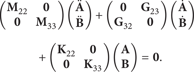
Then, we will get the dynamic equation of the system written in compact form as

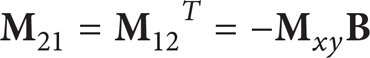
where

where
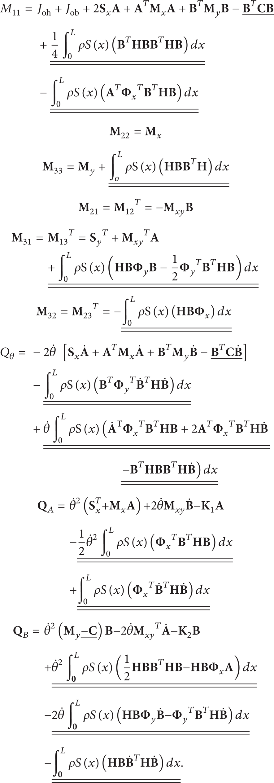
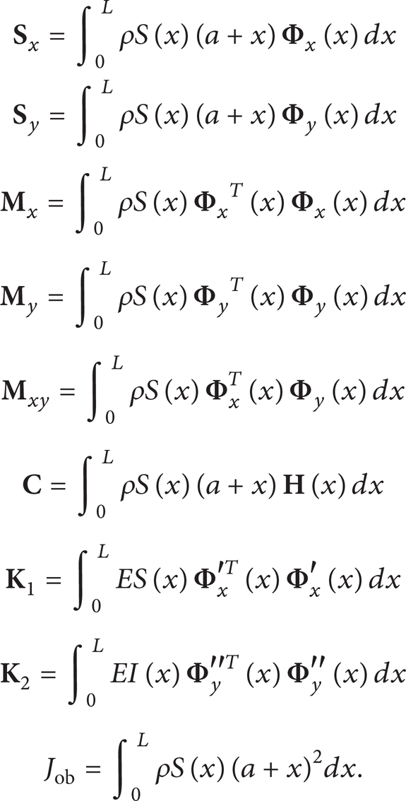
Equation (11) is the rigid-flexible coupling dynamic equation of the system. The parts with single underline in (13) are called the one-order coupling terms. The parts with double underlines in (13) are called the high-order coupling terms. If without the large overall motion, (11) can be degenerated as the structure dynamic equation. Actually, (11) contains four different models: the high-order approximation coupling (HOAC) model with large overall motion, the first-order approximation coupling (FOAC) model with large overall motion, the zero-order approximation coupling (ZOAC) model with large overall motion, and the structure dynamic model without large overall motion. The constant matrices in (13) can be expressed as
3. First-Order Approximation Coupling (FOAC) Model
When evolving the kinetic energy expression, since the coupling deformation w c (x, t) is the second-order amount of the transversal deformation w2(x, t), some high-order amount respected to w c (x, t) can be ignored. Thus, the parts with double underlines in (13) can be ignored. So, (11) can be transferred as another form
where


Equation (15) is calledthe FOAC dynamic equations. The parts with single underline in (16), (23), and (24) are called one-order coupling terms. In the traditional ZOAC model, these parts are always ignored.
3.1. Transversal Bending Vibration Analysis Ignoring Longitudinal Deformation Effect
The transversal bending vibration analysis will be studied in this section. For simplifying analysis, the angular speed of the large overall motion is assumed to be constant as

For convenience of discussion, dimensionless parameters are used in the present analysis and they are defined as

where T = (ρS0L4/EI0)1/2 and S0 = b2h2, I0 = (1/12)b23h2. And δ, γ, α, and β will denote the hub radius ratio, the angular speed ratio, the width ratio, and the height ratio, respectively.
The dimensionless form of the free vibration equation is finally obtained by using the dimensionless variables and parameters defined in (27)

where

Let

where λ is imaginary, ω is the dimensionless natural frequency, and Θ is a constant column matrix.
Table 1 shows the dimensionless natural frequencies of the uniform beam without hub in the transversal bending vibration under different γ, where δ = 0, and α = β = 1, truncate the first four modes when calculating. From Table 1, we can see that the dimensionless natural frequencies here are the same as the results of paper [13], using another modeling method. That proves the correctness of this model. So we will truncate the first four modes when calculating in the following analysis. Additionally, we can see that the dimensionless natural frequencies increase as the angular speed ratio γ increases.
The dimensionless natural frequencies of the uniform beam in transversal bending vibration with different γ (δ = 0, α = β = 1).

In Table 2, two models are compared, one is the FOAC model in this paper, and the other is the traditional ZOAC model (without the single underline parts). Also, the beam is considered to be a uniform one for simplifying analysis, where δ = α = β = 1. From (28), we can find that the two models are same when γ = 0. So the natural frequencies are equal when γ = 0. When γ increasing, the natural frequencies of the two models become discriminative. When the angular speed of the large overall motion is low (γ = 2), the natural frequencies of the two models have a small distinction. But when the large overall motion is at high speed, the natural frequencies of the ZOAC model will be imaginary, which is impractical, while the natural frequencies of the FOAC model are still real. So we can say that the traditional ZOAC model without the coupling deformation is inapplicable when the large overall motion of the beam is at high speed.
The dimensionless natural frequencies of the uniform beam in the transversal bending vibration with different models (δ = α = β = 1).

Table 3 shows the dimensionless natural frequencies of the tapered beam in the transversal bending vibration under different δ, where α = β = 0.5. It is obvious that the dimensionless natural frequency is proportional to the hub radius ratio δ, especially when the large overall motion is at high speed.
The dimensionless natural frequencies of the tapered beam in the transversal bending vibration with different δ (α = β = 0.5).

Table 4 shows the first dimensionless natural frequencies of the tapered beam with different α when δ = β = 1. As we can see, the first natural frequency is in inverse proportion to the width ratio α. When α changes from 0 to 0.3, the first natural frequency will have a great change. Compared to the change of the first natural frequency when γ = 2, the change of the first natural frequency is much smaller when γ = 10.
The first dimensionless natural frequencies in the transversal bending vibration with different α (δ = β = 1).
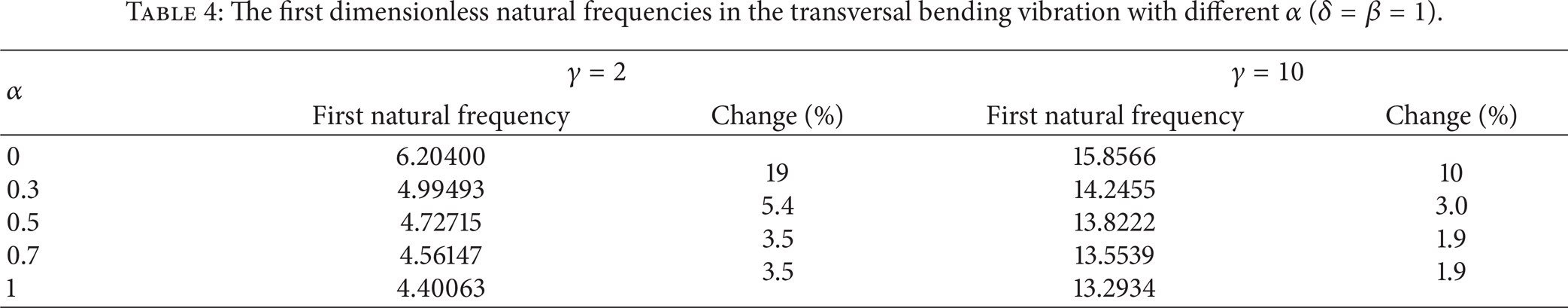
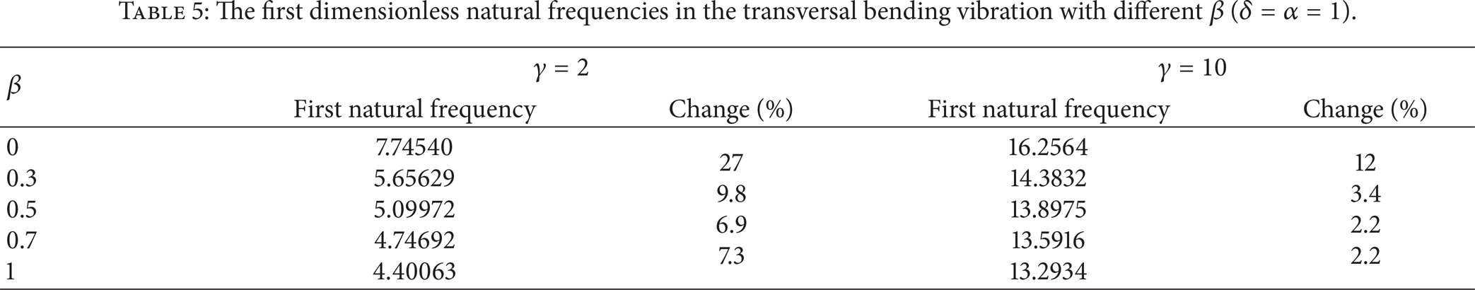
Table 5 shows the first dimensionless natural frequencies of the tapered beam with different β when δ = α = 1. Also, the first natural frequency is in inverse proportion to the height ratio β. As we can see, the changes of the first natural frequency under different β have the same variation as the changes of the first natural frequency under different α.
The first dimensionless natural frequencies in the transversal bending vibration with different β (δ = α = 1).
3.2. Transversal Bending Vibration Analysis Including Longitudinal Deformation Effect
The transversal bending vibration analysis including longitudinal deformation effect will be studied in this section. Also, the angular speed of the large overall motion is assumed to be constant as
Other dimensionless parameters are defined as

where ∊ is proportional to the length to thickness ratio of a beam, called the slenderness ratio. Now, the dimensionless form of the free vibration equation can be obtained as

where


Equation (31) can also be transformed into the following form:
where

Let

where σ is the complex eigenvalue.
Table 6 shows the comparison of the first transversal natural frequencies with and without longitudinal deformation effect when α = β = 0.5 and ∊ = 70. The value of ∊ = 70 guarantees the assumptions of Euler-Bernoulli beam. From (35), we can see that matrix
Comparison of the first transversal natural frequencies with and without longitudinal effect (α = β = 0.5, ∊ = 70).

4. High-Order Approximation Coupling (HOAC) Model
Equation (11) is the rigid-flexible coupling dynamic equation of the system, which is also called the high-order approximation coupling (HOAC) dynamic equation. The parts with double underlines in (13) are called the high-order coupling terms. These terms are always ignored in the FOAC dynamic equations for convenience. But they will have a great influence on the dynamics of the system with large deformation. Here, two examples will be given to approve it.
4.1. Beam Undergoing Prescribed Translation and Rotation
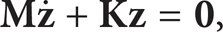
A tapered beam made of aluminum with the dimensions and material properties given in Table 7 is used. The boundary conditions of a cantilever beam are used in the simulations. And the torque applied at the hub τ can be expressed as

where T = 2s.
Data of the hub-tapered beam system.
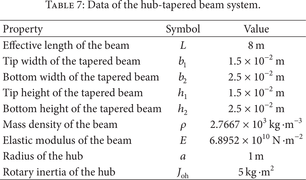
Figure 4(a) gives the tip deformations of the tapered beam with HOAC model and FOAC model when τ0 = 36 N·m. When the torque is applied on the hub, the max tip deformation is 0.56 m, which is only a small deformation to the effective length of the beam. In this case, the tip deformations of the HOAC model and the FOAC model are exactly coincidental, while Figure 4(b) gives the tip deformations of the two models when τ0 = 136 N·m. When the torque applying on the hub, the max tip deformation of the HOAC model reached 2.32 m, this is obviously a large deformation to the effective length of the beam. So, in this case, the result of the FOAC model becomes divergent as shown in Figure 4(b). On the other hand, the result of the HOAC model is still convergent. Then, we can say that the FOAC model is inapplicable in the situation of large deformation, while the HOAC model is applicable. That is because the high-order terms with double underlines respected to w c (x, t) were ignored in the FOAC modeling.

The tip deformation of the tapered beam.
The deformation of the tapered beam in the rotating frame o′ –

The deformation in rotating frame.
The motion in inertial reference frame.
In order to research the dynamic response of the tapered beam, two ratios are defined here, the width ratio R b = b1/b2 and the height ratio R h = h1/h2. And two situations are assumed here, on the assumption that the weight of the tapered beam stays invariable.
Suppose the height of the beam keeps uniform, as h1 = h2 = 0.02 m. Then, we will get

Suppose the width of the beam keeps uniform, as b1 = b2 = 0.02 m. Then, we will get

Figure 7 gives the max tip deformations and the response frequency of the tapered beam with different R b and R h . It is apparent that the max tip deformation increases as R b and R h increases, while the response frequency decreases as R b and R h increases. Also, we will find that the change of R b will have a greater influence on the dynamics of the tapered beam on our assumption (the weight of the tapered beam keeps invariable). But in any case, all R b and R h will have a great influence on the dynamics of the tapered beam.

The dynamic impact of R b , R h .
4.2. Single Pendulum with Gravity
To illustrate the effect of large deformation, a flexible tapered pendulum with free falling is investigated as shown in Figure 8. The pendulum is assumed to fall under the effect of gravity.

The flexible tapered pendulum.
To a flexible tapered pendulum with free falling, the gravitational potential energy should be included. So, the gravitational potential energy will be added to the system potential energy

where

Since the FOAC model could not be used in the large deformation problems, paper [16] investigated the application of an absolute nodal coordinate formulation in the coupling dynamics of flexible beams with large deformation. The simulation of a flexible pendulum indicated that the absolute nodal coordinate formulation is suited for the beams with large deformation, while the FOAC model cannot be used in that case. Here, we will simulate the example of Figure 4 in paper [16] by using the HOAC model. In reference to paper [16], the flexible pendulum is a uniform one, ρ = 2.76667 × 10³ kg·m−3, L = 1.8 m, S(x) = 2.5 × 10⁻⁴ m2, I(x) = 1.3 × 10⁻⁹ m4, and E = 6.8952 × 10⁹ N·m−2.
Figure 9 shows the tip deformation of the flexible pendulum with large deformation. As we can see, the result of the FOAC model is divergent, while the result of the HOAC model is nearly the same as the result of paper [16]. This proves the validity of the HOAC model and the applicability in the large deformation situation. As we know, the absolute nodal coordinate method cannot distinguishthe rigid body motion from the elastic deformation of the flexible body. Small deformation problems also should be treated as large deformation problems, while the FOAC model can only deal with the small deformation problems. However, the HOAC model proposed in this paper can make up for the deficiency of those two methods.

The tip deformation of the uniform pendulum.
To further prove the applicability of the HOAC model in the large deformation situation, a quiet flexible tapered pendulum will be studied here. The dimensions and material properties are still as shown in Table 7, except E = 6.8952 × 10⁵ N·m−2, a = 0 m.
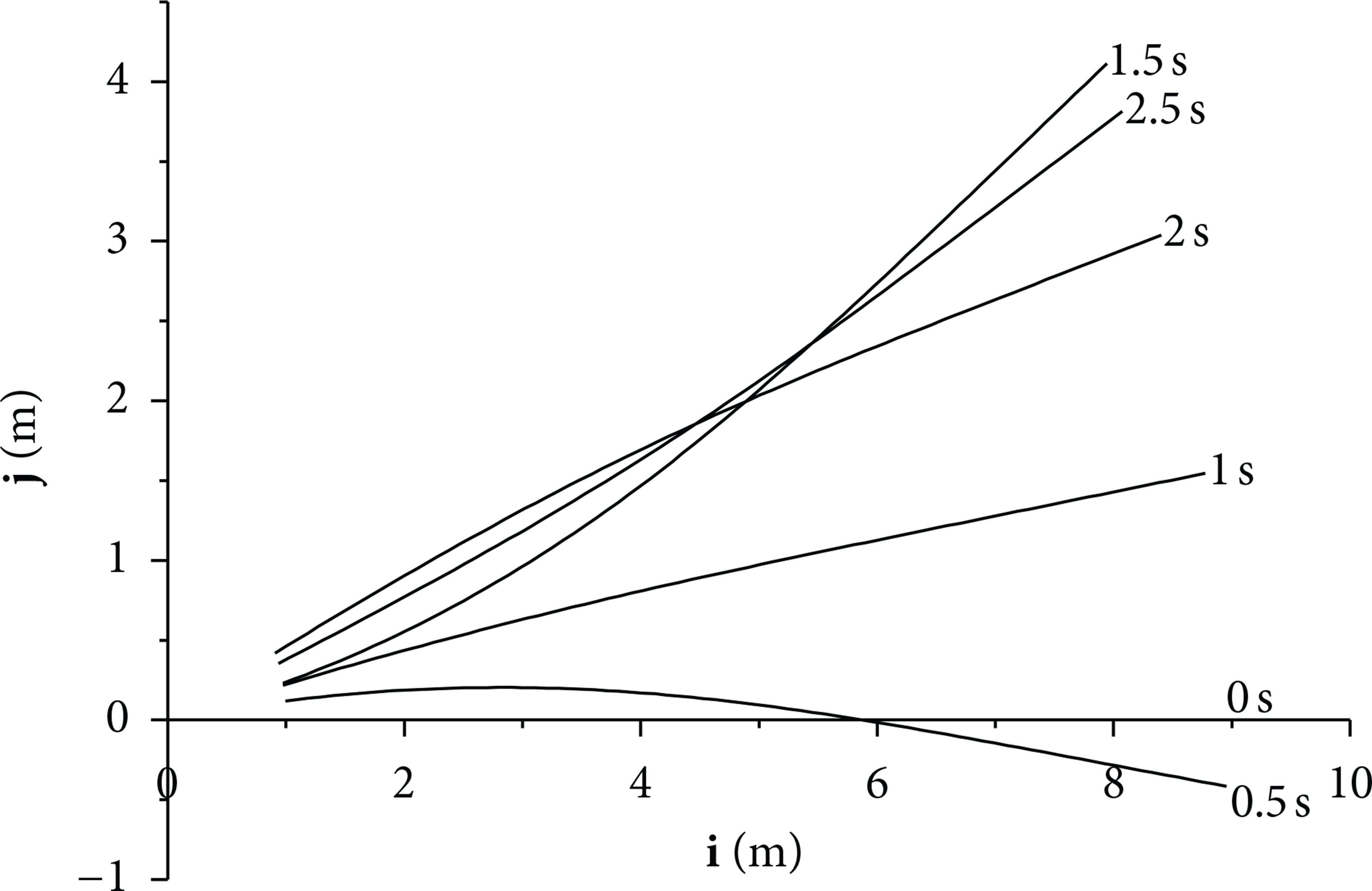
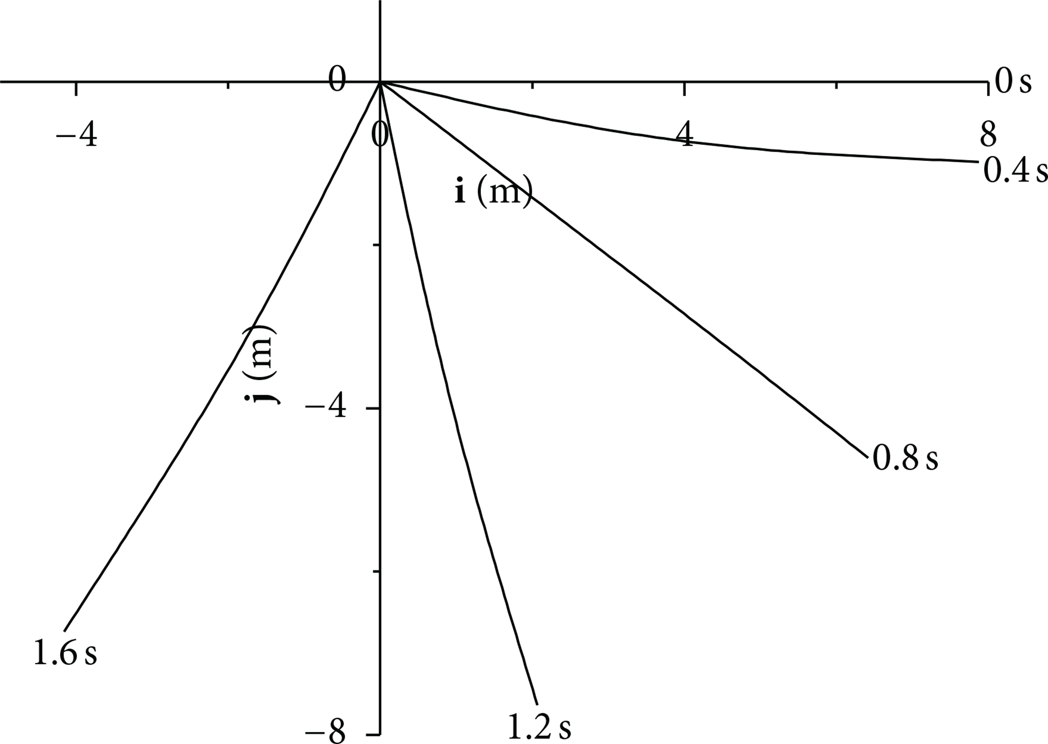
Figure 10 shows the deformed shape of the tapered pendulum with HOAC model at different time steps when E = 6.8952 × 10⁵ N·m−2. As we can see, the deformation is very large at any time step. If we use the FOAC or ZOAC models, the simulation will be divergent.

The deformed shape at different times when E = 6.8952 × 10⁵ N·m−2.
Figure 11 shows the energy change of the tapered pendulum. Curve 1 is the kinetic energy, curve 2 is the elastic potential energy, curve 3 is the gravitational potential energy, and curve 4 is the total energy. Obviously, as the pendulum falls, the kinetic energy increases at the beginning stage. But when the pendulum passes someplace, the kinetic energy will decrease. Also, the elastic potential energy changes the same law as the kinetic energy, while the gravitational potential energy decreases before the pendulum falls to the lowest point. When the pendulum passes the lowest point, the gravitational potential energy will increase. Anyway, the total energy keeps invariant at any time.

The energy change of the tapered pendulum when E = 6.8952 × 10⁵ N·m−2.
Figure 12 shows the deformed shape of the tapered pendulum with HOAC model at different time steps when E = 6.8952 × 10¹⁰ N·m−2. As we can see, the deformation is very small at any time step. So, the elastic potential energy is almost 0 (Figure 13). However, the elastic potential energy is very significant when E = 6.8952 × 10⁵ N·m−2. Also, there are some differences between the kinetic energies when E = 6.8952 × 10⁵ N·m−2 and E = 6.8952 × 10¹⁰ N·m−2. The kinetic energy change is more complex when large deformation occurs.
The deformed shape at different times when E = 6.8952 × 10¹⁰ N·m−2.

The energy change when E = 6.8952 × 10⁵ N·m−2 and E = 6.8952 × 10¹⁰ N·m−2.
5. Conclusion
A new rigid-flexible coupling model of a hub-tapered beam system, which is also called the high-order approximation coupling (HOAC) model, was established in this paper. The HOAC model could not only be used in the case of small deformation, but also in the case of large deformation, while the previous FOAC model could only be used in the case of small deformation. Based on the HOAC model, the motion and the dynamic response of the tapered beam were studied.
Also, the natural frequencies of the FOAC model were studied through the transversal bending vibration analysis. The dimensionless natural frequencies were shown to increase as the angular speed ratio γ and the hub radius ratio δ increased. However, they decreased as the width ratio α and the height ratio β increased. When the large overall motion was at very high speed, the longitudinal deformation would also have a significant influence on the transversal bending vibration.
Footnotes
Acknowledgments
This work was financially supported by the National Natural Science Foundation of China (nos. 11302192, 10772085, 11132007, and 11272155) and the 333 Project of Jiangsu Province (BRA2011172), for which the authors are grateful.