Reduced-Order Computational Model for Low-Frequency Dynamics of Automobiles

Abstract

A reduced-order model is constructed to predict, for the low-frequency range, the dynamical responses in the stiff parts of an automobile constituted of stiff and flexible parts. The vehicle has then many elastic modes in this range due to the presence of many flexible parts and equipment. A nonusual reduced-order model is introduced. The family of the elastic modes is not used and is replaced by an adapted vector basis of the admissible space of global displacements. Such a construction requires a decomposition of the domain of the structure in subdomains in order to control the spatial wave length of the global displacements. The fast marching method is used to carry out the subdomain decomposition. A probabilistic model of uncertainties is introduced. The parameters controlling the level of uncertainties are estimated solving a statistical inverse problem. The methodology is validated with a large computational model of an automobile.

1. Introduction

Automobiles are complex three-dimensional dynamical systems for which the prediction of vibration and acoustic behavior requires highly advanced computational tools. Automobiles are made up of stiff parts such as hollow bodies and flexible parts such as panels and many pieces ofequipment. This kind of structure presents in the low-frequency (LF) band [5, 200] Hz a very large number of elastic modes (for instance 1,000). The flexible parts of an automobile as well as equipments are not fully defined during the advanced design phase; that is not the case for the stiff parts. During this draft design, the flexible panels and equipments are not yet completely defined. A vibration analysis in the LF range is performed during the draft design. Since a noise and vibration analysis in the LF range has to be performed in order to assess the advanced design, it is important to construct a robust computational model for predicting the LF vibrations of the stiff parts with respect to the design variations of the flexible parts and the equipments, and with respect to uncertainties. The objective of this paper is to present a novel approach for constructing an adapted reduced-order model, which does not use the elastic modes but which use another vector basis, in order to predict, in the LF range, the responses of the stiff parts. In addition, it should be noted that the multiplication of equipments and the refinement of meshes yield very large computational model, more than 8 millions of degrees of freedom (DOF). This aspect increases the necessity to build reduced-order models with a low dimension and which remain predictive in the LF band for the stiff parts.

For automobiles, in the LF band, there are numerous elastic modes with predominant local displacements (displacements at a specific location on the vehicle) induced by the presence of flexible panels and equipments and there are a few elastic modes with predominant global displacements (displacements in phase over all the vehicle). In this LF band, each elastic mode shows global and local contributions, and it is difficult to define an objective criterium in order to isolate the elastic modes which have predominant global displacements which would allow us to construct a reduced-order model to predict the responses of the stiff parts in the LF band.

In the LF band, the vibration analysis was the subject of numerous research. The fundamentals and in particular the technique of modal analysis are presented in the textbooks [1–5]. The main techniques of dynamic substructuring are developed in the books and papers [4–16]. All these techniques are very well adapted for the construction of a reduced-order model in the LF band, when the resonances are relatively well separated (low-modal density).

This paper deals with the dynamical analysis of complex automobile structures for which there are global elastic modes coupled to numerous local elastic modes in the LF band. The construction of a global displacements basis, independently of the frequency band analyzed, has been the subject of a few researches. Most of them are based on a spatial filtering of the “short” spatial wavelengths. In signal processing of experimental data, this filtering is done using regularization techniques [17], image processing [18]. In the context of the use of computational model built using the finite element (FE) method, the construction of the global displacements basis can be carried out using, for instance, (1) an extraction technique of the family of eigenvectors related to the frequency mobility matrix, (2) a direct extraction of the family of the elastic modes, and (3) the technique of the lumped masses. In the static condensation method of Guyan, the masses are concentrated in some nodes (master nodes) and the inertia is neglected. The choice of the master nodes is difficult [19–21]. The techniques related to the concentrated mass method has been the subject of numerous research, particularly with regard to the convergence of these methods [22–24].

There are three objectives in this paper: (1) the first one is the construction of a reduced-order model adapted to the predictions of the LF responses of the stiff parts of the structure in presence of numerous flexible parts and equipments; such a construction requires the introduction of an adapted vector basis related to the global displacements; (2) the second one is the construction of a stochastic reduced-order model to take into account both the system-parameter uncertainties and the model uncertainties induced by the irreducible errors introduced by neglecting the local displacements contributions and the other modeling errors; (3) the last one concerns the application of this method on an automobile represented by a very large computational model. To solve the first objective, the recent method proposed in [25] is used and adapted to the present framework of the LF vibration analysis of automobiles [26]. This method introduces a nonusual basis of the admissible space of global displacements. The construction of this basis requires the decomposition of the domain of the structure in subdomains. This subdomain decomposition is performed by using the fast marching method which is extended for complex computational model [26]. The reduced-order computational model is then constructed with this vector basis deduced from the computational model. To take into account uncertainties, a stochastic reduced-order model is introduced. These uncertainties are due to (i) the system-parameter uncertainties and the model uncertainties induced by the modeling errors in the computational model and (ii) the errors induced in neglecting the elastic modes with predominant local displacements. These sources of uncertainties are modeled using the nonparametric probabilistic approach of uncertainties [27, 28]. For an automobile, the large computational model of automobile has numerous uncertainties associated with the system-parameter uncertainties and the modeling errors introduced during the construction of the computational model. This has been clearly established in previous works (see [29–31]).

Dispersion parameters related to uncertainties are introduced in the stochastic reduced-order computational model. These parameters are identified using the maximum likelihood method for which the experimental data come from previous works [29]. The methodology proposed has been validated in [26] for a simplified model of an automobile (most of the equipments and flexible panels, which induced numerous local elastic modes, are removed from the computational model). In this paper, a complete validation of the methodology is presented for a complete computational model of an automobile. In Section 2, the reference nominal computational model is built. Section 3 is devoted to a summary of the construction of the reduced-order model with uncertainties. Finally, Section 4 deals with the application to an automobile.

2. Nominal Computational Model and Classical Reduced-Order Model (CROM)

The frequency response functions are predicted in the frequency band of analysis, ℬ = [ω_min, ω_max], with 0 < ω_min, for a damped structure occupying a domain Ω. The nominal computational model is constructed with the finite element method. Let 𝕌(ω) be the complex vector of the m DOF in displacements of the structure. Let [𝕄], [𝔻], and [𝕂] be the mass, the damping, and the stiffness matrices. It is assumed that there are no rigid body displacements. Consequently, [𝕄], [𝔻], and [𝕂] are positive-definite symmetric (m × m) real matrices. Let 𝕗(ω) be the vector which discretizes the external forces. For all ω fixed in ℬ, complex vector 𝕌(ω) is the unique solution of the complex matrix equation,

$\mathrm{\hspace{0.17em}\hspace{0.17em}}(-{\omega }^{\mathrm{2}}\left[𝕄\right]+i\omega \left[𝔻\right]+\left[𝕂\right])𝕌\left(\omega \right)=𝕗\left(\omega \right).$

(1)

Let ω_α be the eigenfrequency of the elastic mode φ_α of the conservative part of the computational model. Introducing λ_α = ω_α², one has

$\mathrm{\hspace{0.17em}\hspace{0.17em}}\left[𝕂\right]{\mathbf{\phi }}_{\alpha }={\lambda }_{\alpha }\left[𝕄\right]{\mathbf{\phi }}_{\alpha }.$

(2)

Then, an approximation 𝕌⁽ⁿ⁾(ω) of 𝕌(ω) at order n is the solution of the classical reduced-order model (CROM) constructed with the elastic modes:

${𝕌}^{\left(n\right)}\left(\omega \right)=\sum _{\alpha =\mathrm{1}}^n\hspace{0.17em}{q}_{\alpha }\left(\omega \right){\mathbf{\phi }}_{\alpha },$

(3)

in which q(ω) = (q₁ (ω), …, q _n (ω)) is the complex vector of the n generalized coordinates, which is the solution of the complex matrix equation:

$\left(-{\omega }^{\mathrm{2}}\left[ℳ\right]+i\omega \mathrm{\hspace{0.17em}\hspace{0.17em}}\left[𝒟\right]+\left[𝒦\right]\right)\mathbf{q}\left(\omega \right)=ℱ\left(\omega \right),$

(4)

in which [ℳ], [𝒟], and [𝒦] are the classical generalized mass, damping, and stiffness matrices, and where ℱ(ω) is the generalized external force.

3. Construction of the Reduced-Order Model (ROM)

In this section, the methodology [26] used to construct the reduced-order model (ROM) with a global displacements basis, and not with the elastic modes, is summarized. This ROM is adapted to the prediction of the FRF in the low-frequency band for the stiff parts of the structure. This ROM is different from the CROM.

Two nonusual eigenvalue problems are introduced for which the solutions provide a basis of the global displacements space and a basis of the local displacements space. The union of these two bases yields a basis of the admissible displacement space [25]. The construction of these two bases is carried out in introducing a spatial filtering which allows us to introduce a kinematic reduction of the kinetic energy while the elastic energy remains exact. The spatial filtering is based on the decomposition of the domain in subdomains. The mean size of the subdomains corresponds to the spatial wavelength cutoff. This decomposition in subdomains is automatically carried out using the fast marching method [26] which is summarized bellow. Finally, a stochastic reduced-order model (SROM) is constructed in implementing the nonparametric probabilistic approach of uncertainties (see [28]) in the ROM in order to take into account both the system-parameter uncertainties and the model uncertainties induced by the modeling errors.

3.1. Decomposition of the Domain in Subdomains

Domain Ω of the structure is decomposed in N subdomains Ω _j , with j belonging to 1, …, N (see Figure 1). For a complex finite element model such as the computational model of an automobile, the automatic construction of domain Ω in subdomains Ω _j , for which a characteristic dimension corresponding to the spatial wavelength cutoff is imposed, is relatively difficult and requires adapted methods. As proposed in [26], this decomposition is carried out using the fast marching method (FMM) introduced in [32, 33].

Figure 1:

Decomposition of Ω in subdomains.

3.1.1. Presentation of the Fast Marching Method

This method allows a front to be propagated in a finite element mesh from a starting point. All the details of the construction of the FMM used in this paper are developed in [26]. Let g _ij be the geodesic distance between the node indexed by i and the node indexed by j. The algorithm can be summarized as follows.

Initialization

• Choose a starting node indexed by 0, and set g₀₀ = 0 (see Figure 2(a)).

• The four neighboring nodes of the starting node are selected such as these nodes are the front and for each neighboring nodes, the geodesic distance, g_0j, is calculated with the starting node (see Figure 2(a)).

• For all the other nodes, put g_0j = + ∞.

Figure 2:

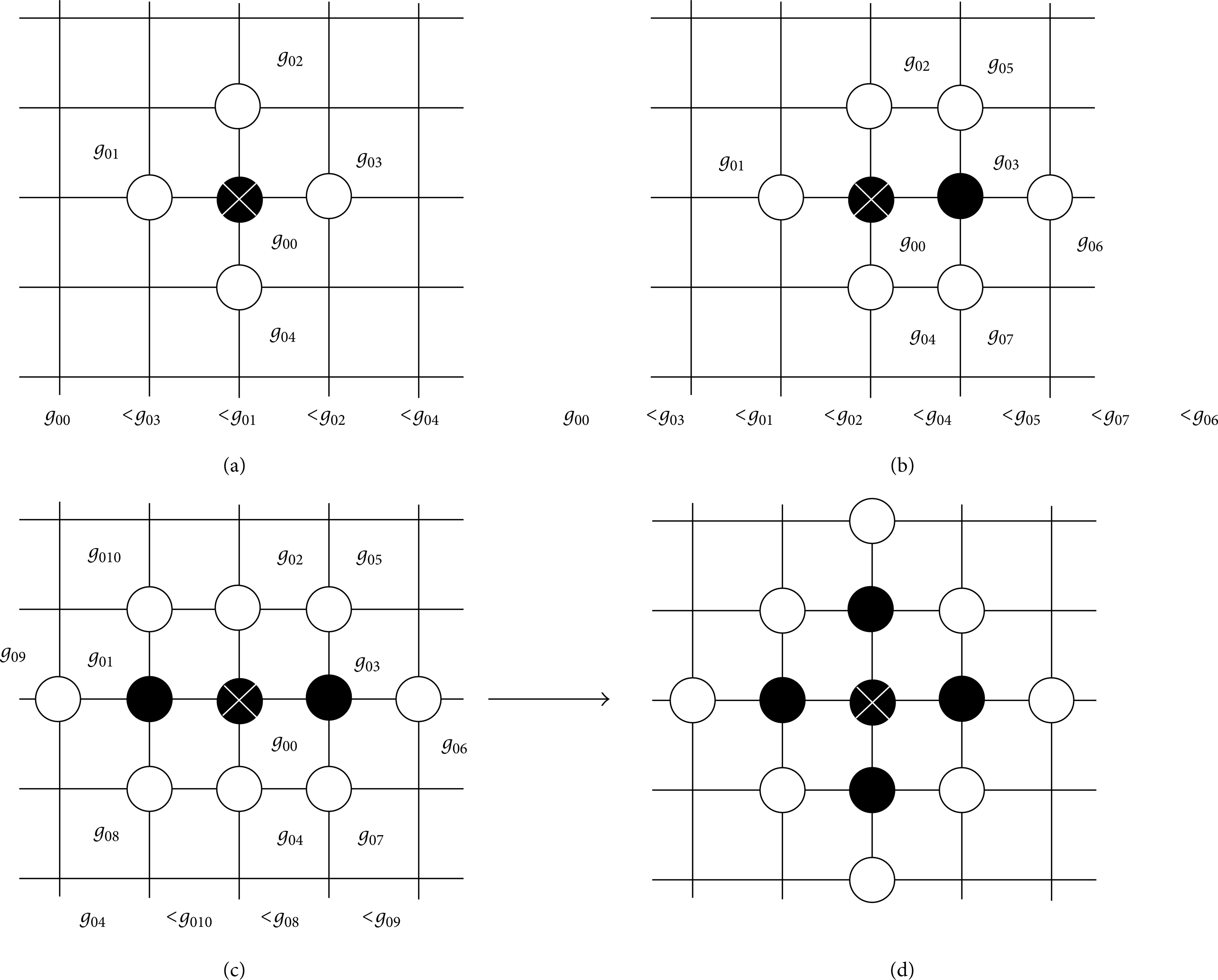
Diagram of the fast marching method: step 1 (a), step 2 (b), step 3 (c), and the last step corresponding to the diagram, step 4 (d).

Loop

• Among the front nodes, select the node with the smallest value of g_0j.

• Remove this node from front nodes and add this node to the subdomain (see Figure 2(b)).

• For each neighboring node of this node, the geodesic distance is calculated or recalculated (if this neighboring node is in front nodes).

The loop is repeated until all the nodes belong to a subdomain (see Figure 2(d)). For the calculation of the geodesic distance, the method used depends on the angle (acute or obtuse) of the finite elements of the mesh [32, 33]. The different cases which can be encountered have been analyzed in [26].

3.1.2. Construction of Subdomains

The subdomains Ω _j of Ω are constructed using the FMM. This construction is performed in two steps. The first one consists in introducing master points which are defined as the points which will be the centers of the subdomains. The second one consists in generating the subdomains using these master points as starting points.

• Selection of the Master Points. In the context of the present developments, heterogeneous structures which exhibit stiff parts and flexible parts are considered. The master points will then be “uniformly” distributed in the stiff parts such that the distance between two neighboring master points is of the order of the smallest wavelength of local displacements which has to be filtered (wavelength cutoff).

• Generation of Subdomains. To construct the subdomains Ω _j using a set of master points, the fronts starting from master points are simultaneously propagated until all the nodes belong to a subdomain. Then, the boundaries of the generated subdomains correspond to the meeting lines of the fronts.

3.2. Construction of Vector Bases for the Global and the Local Displacements Spaces

In this section, the projection operator h ^r which will be applied to the mass matrix in order to obtain the spatial filtering is introduced. Let x → u(x) be any displacement field defined in Ω and belonging to the admissible displacement space. For all displacement field u belonging the admissible displacement space, operator h ^r is defined by

$\left\{h^r\left(\mathbf{u}\right)\right\}\left(\mathbf{x}\right)=\sum _{j=\mathrm{1}}^N\hspace{0.17em}{𝕀}_{{\Omega }_j}\left(\mathbf{x}\right)\frac{\mathrm{1}}{m_j}{\int }_{{\Omega }_j}\hspace{0.17em}\rho \left({\mathbf{x}}^{\prime }\right)\mathbf{u}\left({\mathbf{x}}^{\prime }\right)d{\mathbf{x}}^{\prime },$

(5)

in which x → 𝕀_{Ω j} (x) = 1 if x belongs to Ω _j and = 0 otherwise. For all j = 1, …, N, m _j is the local mass defined by $m_j={\int }_{{\Omega }_j}\hspace{0.17em}\rho (\mathbf{x})d\mathbf{x}$ , and ρ(x) is the mass density. The displacement field h ^r (u) corresponds to a kinematic reduction which will be used to calculate the kinetic energy. As it can be seen, h ^r (u) averages the displacement field u over each subdomain Ω _j with respect to the mass density. This operator will allow a given spatial filtering to be obtained and a vector basis of the global displacements space to be calculated.

Let h ^c (u) be the complementary operator defined by

$h^c\left(\mathbf{u}\right)=\mathbf{u}-h^r\left(\mathbf{u}\right).$

(6)

This operator will allow a basis of the local displacements to be calculated.

Let [H ^r ] be the (m × m) matrix of the projection operator h ^r relative to the finite element discretization of the computational model. The projected mass matrix denoted by [𝕄 ^r ], of the mass matrix [𝕄], is then written as

$\mathrm{\hspace{0.17em}\hspace{0.17em}}\left[{𝕄}^r\right]={\left[H^r\right]}^T\left[𝕄\right]\left[H^r\right].$

(7)

It can be proven that the rank of matrix [𝕄 ^r ] is 3N. To obtain the spatial filtering and thus, to construct the vector basis of the global displacements space, the mass matrix [𝕄] is replaced in the generalized eigenvalue problem [𝕂]φ_α = λ_α[𝕄]φ_α by the projected mass matrix [𝕄 ^r ] defined by (7). The following generalized eigenvalue problem, called the global spectral problem, is then obtained:

$\mathrm{\hspace{0.17em}\hspace{0.17em}}\left[𝕂\right]{\mathbf{\phi }}_{\alpha }^g={\lambda }_{\alpha }^g\left[{𝕄}^r\right]{\mathbf{\phi }}_{\alpha }^g,$

(8)

in which the positive eigenvalue λ_α ^g is called the global eigenvalue and where ${\mathit{\varphi }}_{\alpha }^g$ is the associated global displacements eigenvector. The family $\{{\mathit{\varphi }}_{\mathrm{1}}^g,\dots ,{\mathit{\varphi }}_{\mathrm{3}N}^g\}$ associated with the 3N ordered positive eigenvalues, λ₁ ^g ≤ · ≤ λ_3N ^g , constitutes a basis of the space of the global displacements space which has the finite dimension3N and which is a subspace of ℝ ^m .

Let [H ^c ] be the (m × m) matrix of the complementary operator h ^c , such that [H ^c ] = [I] – [H ^r ], where [I] is the (m × m) identity matrix. Matrix [H ^c ] is then used to construct the complementary mass matrix [𝕄 ^c ] such that

$\mathrm{\hspace{0.17em}\hspace{0.17em}}\left[{𝕄}^c\right]={\left[H^c\right]}^T\left[𝕄\right]\left[H^c\right].$

(9)

It can be proven that the rank of matrix [𝕄 ^c ] is m – 3N. As previously done, the mass matrix [𝕄] is replaced by the complementary mass matrix [𝕄 ^c ] in (2) and yields the following generalized eigenvalue problem, called the local spectral problem:

$\mathrm{\hspace{0.17em}\hspace{0.17em}}\left[𝕂\right]{\mathbf{\phi }}_{\beta }^{\ell }={\lambda }_{\beta }^{\ell }\left[{𝕄}^c\right]{\mathbf{\phi }}_{\beta }^{\ell },$

(10)

in which the positive eigenvalue λ_β^ℓ is called the local eigenvalue and ${\mathit{\varphi }}_{\beta }^{\ell }$ is the associated local displacements eigenvector. The family $\{{\mathit{\varphi }}_{\mathrm{1}}^{\ell },\dots ,{\mathit{\varphi }}_{m-\mathrm{3}N}^{\ell }\}$ associated with the m – 3N ordered positive eigenvalues, λ₁^ℓ ≤ … ≤ λ_{m – 3N}^ℓ, constitutes a basis of the space of the local displacements space which has the finite dimension m – 3N and which is a subspace of ℝ ^m .

It is proven that the families $\{{\mathit{\varphi }}_{\mathrm{1}}^g,\dots ,{\mathit{\varphi }}_{\mathrm{3}N}^g\}$ and $\{{\mathit{\varphi }}_{\mathrm{1}}^{\ell },\dots ,{\mathit{\varphi }}_{m-\mathrm{3}N}^{\ell }\}$ are not orthogonal but are algebraically independent and that their union, $\{{\mathit{\varphi }}_{\mathrm{1}}^g,\dots ,{\mathit{\varphi }}_{\mathrm{3}N}^g,{\mathit{\varphi }}_{\mathrm{1}}^{\ell },\dots ,{\mathit{\varphi }}_{m-\mathrm{3}N}^{\ell }\}$ , is a basis of ℝ ^m .

If the computational model is developed with a commercial software, these two spectral problems can be solved by the double projection method presented in [25], in order to avoid having to export the mass matrix [𝕄] outside the software.

3.3. Construction of the ROM

This section deals with the ROM constructed using only the global displacements basis which is suitable for the predictions of the frequency responses of the structural stiff parts in the LF band. As explained in Section 1, we are interested in the frequency responses in the stiff part and in the low-frequency band ℬ, for which the global displacements are dominant with respect to the local displacements. The reduced-order model at order n _g < n, adapted to this case, is constructed in introducing the projection 𝕌^{(n _g )}(ω) of 𝕌(ω) on the subspace spanned by the global displacements eigenvectors ${\mathit{\varphi }}_{\mathrm{1}}^g,\dots ,{\mathit{\varphi }}_{n_g}^g$ . We then have the following ROM:

$\begin{array}{c}{𝕌}^{\left(n_g\right)}\left(\omega \right)=\sum _{\alpha =\mathrm{1}}^{n_g}\hspace{0.17em}{q}_{\alpha }^g\left(\omega \right){\mathit{\varphi }}_{\alpha }^g,\\ \left(-{\omega }^{\mathrm{2}}\left[M^{gg}\right]+i\omega \left[D^{gg}\right]+\left[K^{gg}\right]\right){\mathbf{q}}^g={\mathbf{f}}^g,\end{array}$

(11)

in which [M ^gg ] = [Φ ^g ] ^T [𝕄][Φ ^g ], [D ^gg ] = [Φ ^g ] ^T [𝔻][Φ ^g ], and[K ^gg ] = [Φ ^g ] ^T [𝕂][Φ ^g ] are full (n _g × n _g ) real matrices, where f ^g (ω) = [Φ ^g ] ^T 𝔽(ω) is a complex vector of dimension n _g and where the (m × n _g ) real matrix [Φ ^g ] is such that $[{\mathrm{\Phi }}^g]=[{\mathit{\varphi }}_{\mathrm{1}}^g·{\mathit{\varphi }}_{n_g}^g]$ .

3.4. Construction of the SROM

As explained above, the nonparametric probabilistic approach of uncertainties is used to construct the SROM. Therefore the matrices [M ^gg ] and [K ^gg ] are replaced by the random matrices [M ^gg ] and [K ^gg ] for which the probability density functions and the generator of independent realizations are given in [27, 28]. The probability density functions of these two random matrices depend on two dispersion parameters (δ _{M ^gg} and δ _{K ^gg} ) which have to be identified using the random frequency responses of the stochastic reference model and the maximum likelihood method. The details of the construction of the SROM are given in [26]. The random frequency response U ^g (ω; δ _{M ^gg} , δ _{K ^gg} ) is constructed with the following SROM:

$\begin{array}{c}{\mathbf{U}}^g\left(\omega ;{\delta }_{M^{gg}},{\delta }_{K^{gg}}\right)=\sum _{\alpha =\mathrm{1}}^{n_g}\hspace{0.17em}{\mathbf{Q}}^{\alpha }\left(\omega ;{\delta }_{M^{gg}},{\delta }_{K^{gg}}\right){\mathit{\varphi }}_{\alpha }^g,\\ \left[{\mathbf{A}}^{gg}\left(\omega \right)\right]{\mathbf{Q}}^g\left(\omega ;{\delta }_{M^{gg}},{\delta }_{K^{gg}}\right)={\mathbf{f}}^g\left(\omega \right),\end{array}$

(12)

in which the random complex matrix [A ^gg (ω)] depends on ω, δ _{M ^gg} , δ _{K ^gg} and is written as

$\left[{\mathbf{A}}^{gg}\left(\omega \right)\right]=-{\omega }^{\mathrm{2}}\left[{\mathbf{M}}^{gg}\left({\delta }_{M^{gg}}\right)\right]+i\omega \left[D^{gg}\right]+\left[{\mathbf{K}}^{gg}\left({\delta }_{K^{gg}}\right)\right].$

(13)

4. Nominal Computational Model and SROM for an Automobile

This section is devoted to the application of the method proposed for the computational model of a complete automobile. This type of computational model is very complex (many types of elements, complex geometry, etc) and is constituted of a very large finite element model (FEM), see Figure 3. In this FEM, all the parts of the real vehicle (seats, dashboard, interior finishes, etc) are modeled. In addition, the FEM mesh is very dense and consists of about 1,300,000 nodes (see Figure 3) and contains many volume elements, surface elements and beam elements. This model has about 8,000,000 DOF. The stiff parts correspond to the hollow bodies which are the frame of the car. The flexible parts are all the panels and the different elements which are fixed on these stiff parts. Therefore, this computational model will exhibit a numerous local elastic modes in the LF band which is for the car under consideration the frequency band ℬ = [0, 120] Hz.

Figure 3:

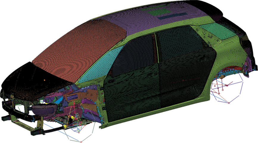
Finite element computational model of an automobile.

4.1. Decomposition of Domain Ω (Complete Surface of the Vehicle) in Subdomains

As explained in Section 3, the first step of the method consists in decomposing the domain Ω in N subdomains Ω _j using the fast marching method. We select 90 master nodes which are uniformly distributed on the stiff parts, which yield N = 90 subdomains. The average distance between two adjacent master nodes characterizes the wavelength cutoff. The repartition of the master nodes is plotted in Figure 4 and the result of the domain decomposition, constructed by the fast marching method, is plotted in Figure 5. As it can be seen in Figure 5, the subdomains constructed with the FMM starting from the master points have a homogeneous size.

Figure 4:

Position of the master nodes.

Figure 5:

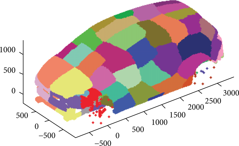
Subdomains constructed by the FMM (one per color).

4.2. Frequency Response Functions of the Nominal Computational Model

The frequency response functions of the nominal computational model defined in Section 2, and called reference FRF, are computed using the classical modal analysis. The first 2165 elastic modes of the FEM have been calculated with Nastran software. The eigenfrequency corresponding to the highest elastic mode is 365 Hz.

The frequency response functions are calculated in the frequency band ℬ = [0, 120] Hz. The structure is subjected to forces and moments applied to the nodes Exc 1 and Exc 2. In each node, there are two forces of 1N in OX and OZ and two moments of 1N × m around OX and OY. These two nodes are located on a stiff part. The responses are calculated in four observation nodes located on the stiff parts. The node Obs 1 is located on the left front of the vehicle, the node Obs 2 on the right front, the node Obs 3 on the left back and the node Obs 4 on the edge of the trunk. All these points are represented in Figure 6. The convergence of the responses in frequency band ℬ, with respect to the number n of elastic modes, has been analyzed in studying the function:

$n⟼\text{Conv}\left(n\right)={\int }_{ℬ}\hspace{0.17em}\mathrm{\hspace{0.17em}\hspace{0.17em}}\sum _{i=\mathrm{1}}^{n_{\text{obs}}}\hspace{0.17em}{\parallel {𝕌}_i^{\left(n\right)}\left(\omega \right)\parallel }^{2}d\omega ,$

(14)

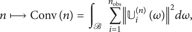
for n ≤ 2,165. In (14), $\parallel {𝕌}_i^{(n)}(\omega )\parallel$ is the Hermitian norm of the displacement vector at node Obs i, and n_obs is the number of observation nodes (n_obs = 4).

Figure 6:

Localization of observation nodes (Obs 1, Obs 2, Obs 3 and Obs 4) and excitation nodes (Exc 1 and Exc 2).

The convergence analysis shows that the convergence is reached for n = 907 elastic modes. The eigenfrequency of the 907th elastic mode is 205 Hz. Consequently, for the frequency band [0, 120] Hz, the reduced-order models are constructed with 907 elastic modes. For the displacement following OZ, the reference FRF are computed for the observation nodes Obs 1, Obs 2, Obs 3, and Obs 4 and are plotted in the Figure 7.

Figure 7:

Reference FRF: modulus in log₁₀-scale of the velocity following OZ for observation nodes: Obs 1 (dashed line), Obs 2 (dotted line), Obs 3 (mixed line), and Obs 4 (solid line).

4.3. Confidence Regions of the Random Frequency Response Functions of the Stochastic Computational Model

The random frequency response functions of the stochastic computational model (called the reference stochastic FRF) for such an automobile are constructed using the nominal reduced-order computational model constructed with the first 907 elastic modes and using the nonparametric probabilistic approach of both the system-parameter uncertainties and the model uncertainties induced by the modeling errors as explained in [29]. This stochastic model of uncertainties is controlled by the dispersion parameters δ _M ^exp and δ _K ^exp of the generalized mass and stiffness matrices. These dispersion parameters have been identified with experimental measurements for an automobile of the same class than the one of the present application for which the same values are used. The statistics of the reference stochastic FRF are estimated using the Monte Carlo method with 1000 independent realizations for solving the stochastic equations. The confidence regions of the reference stochastic FRF, corresponding to a probability level of 0.95, are estimated for observation nodes Obs 1, Obs 2, Obs 3 and Obs 4 and are plotted in Figures 8, 9, 10 and 11 (gray region).

Figure 8:

Confidence region (gray region) of the reference stochastic FRF for observation node Obs 1.

Figure 9:

Confidence region (gray region) of the reference stochastic FRF for observation node Obs 2.

Figure 10:

Confidence region (gray region) of the reference stochastic FRF for observation node Obs 3.

Figure 11:

Confidence region (gray region) of the reference stochastic FRF for observation node Obs 4.

4.4. Global and Local Displacements Eigenvectors

The local displacements eigenvectors and the global displacements eigenvectors are constructed using the method of double projection as explained in [25, 26]. Matrix [H ^r ] is constructed with N = 90 subdomains. Consequently, the maximum value of n _g is 3 × 90 = 270, and the maximum value of n_ℓ is 907 – 270 = 637. For the frequency band [0, 120] Hz, a convergence analysis of the frequency response functions, constructed with the reduced-order model (see (11)), has been carried out in function of the number n _g of global displacements eigenvectors. For that, the following error function is introduced:

$n_g⟼\text{Error}\left(n_g\right)\hspace{0.17em}=\frac{{\int }_{ℬ}{\sum }_{i=\mathrm{1}}^{n_{\text{obs}}}{\parallel {𝕌}_i^{\left(n_g\right)}\left(\omega \right)-{𝕌}_i^{\left(n\right)}\left(\omega \right)\parallel }^2\hspace{0.17em}d\omega }{{\int }_{ℬ}{\sum }_{i=\mathrm{1}}^{n_{\text{obs}}}{\parallel {𝕌}_i^{\left(n\right)}\left(\omega \right)\parallel }^2\hspace{0.17em}d\omega },$

(15)

where 𝕌 _i ⁽ⁿ⁾(ω) is relative to the reference FRF calculated with n = 907 for observation Obs i and 𝕌 _i ^{(n _g )}(ω) is the frequency response function at the same node calculated with the n _g global displacements eigenvectors (see (11)).

Figure 12 displays function n _g → Error (n _g ) and shows that a reasonable convergence is reached for n _g = 50. There are n_ℓ = 382 local displacements eigenvectors in the frequency band [0, 120] Hz. The distributions of the global eigenvalues and the distribution of the local eigenvalues are plotted in Figure 13 which shows that the global displacements eigenvectors are interlaced with a very large number of local displacements eigenvectors.

Figure 12:

Graph of function n _g → Error (n _g ).

Figure 13:

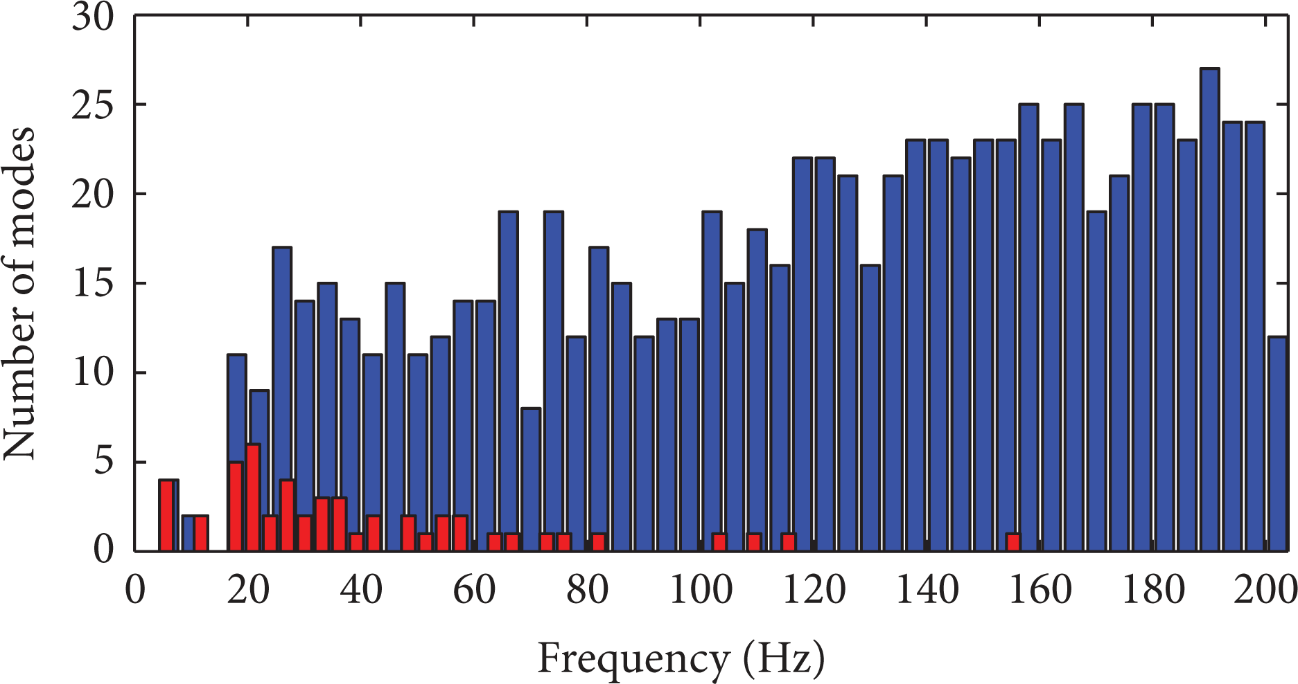
Distribution of the number of global displacements eigenvalues (red histogram) and distribution of the number of local displacements eigenvalues (blue histogram) expressed in terms of frequency in Hz.

4.5. Frequency Response Functions Calculated with the ROM

In this section, for the four observations and for the frequency band [0, 120] Hz, we compare the frequency response functions calculated with the reduced-order model constructed with the first 50 global displacements eigenvectors (see (11) with n _g = 50), with the reference FRF (constructed with the classical reduced-order model on the basis of the first 907 elastic modes, see (1) and (3) with n = 907). In addition, in order to show the gain obtained on the dimension of the reduced-order model when the global displacements eigenvectors are used with respect to the classical reduced-order model constructed with elastic modes, we show the frequency response function calculated with the first 50 elastic modes. The results are displayed in Figures 14, 15, 16 and 17. It can be seen that the reduced-order model constructed with 50 global displacements eigenvectors gives a reasonable good prediction of the reduced-order model constructed with 907 elastic modes. There is an important gain on the dimension of the reduced-order model. The differences which appear will be taken into account by the stochastic model presented in the next section.

Figure 14:

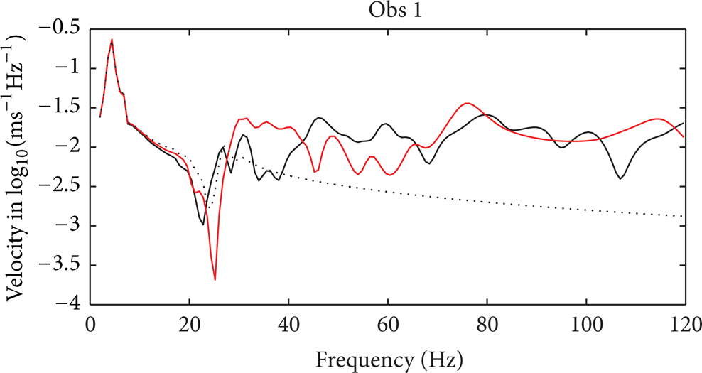
Modulus in log₁₀-scale of the frequency response function in velocity for observation node Obs 1. Reference FRF (black solid line). Classical reduced-order model with the first 50 elastic modes (black dashed line). Reduced-order model with the first 50 global displacements eigenvectors (red thick line).

Figure 15:

Modulus in log₁₀-scale of the frequency response function in velocity for observation node Obs 2. Reference FRF (black solid line). Classical reduced-order model with the first 50 elastic modes (black dashed line). Reduced-order model with the first 50 global displacements eigenvectors (red thick line).

Figure 16:

Modulus in log₁₀-scale of the frequency response function in velocity for observation node Obs 3. Reference FRF (black solid line). Classical reduced-order model with the first 50 elastic modes (black dashed line). Reduced-order model with the first 50 global displacements eigenvectors (red thick line).

Figure 17:

Modulus in log₁₀-scale of the frequency response function in velocity for observation node Obs 4. Reference FRF (black solid line). Classical reduced-order model with the first 50 elastic modes (black dashed line). Reduced-order model with the first 50 global displacements eigenvectors (red thick line).

4.6. Random Frequency Response Functions Calculated with the SROM

The objective of this section is to compare (1) the confidence regions of reference stochastic FRF with (2) the confidence regions of the random frequency response functions calculated with the stochastic reduced-order computational model. This stochastic reduced-order computational model is constructed with the global displacements eigenvectors, and the level of uncertainties is induced by two sources of uncertainties. The first source corresponds to the level of uncertainties introduced in the reference stochastic computational model. The second source is induced by the use of the global displacements eigenvectors without using the local displacements eigenvectors for constructing the reduced-order model. This second source of uncertainties is taken into account with the nonparametric probabilistic approach of uncertainties similarly to the approach used in [29]. In this section, the total level of uncertainties induce by the two sources is globally identified by the maximum likelihood method for which the “experiments” are the confidence regions of reference stochastic FRF.

The deterministic damping matrix of the reduced-order model, constructed with the first 50 global displacements eigenvectors, is reused. The first step consists in calculating the optimal values δ M gg opt and δ K gg opt of the dispersion parameters of the random matrices [M gg (δ M gg )] and [K gg (δ K gg )] using the maximum likelihood method as explained above. The likelihood function (δ M gg , δ K gg ) → L (δ M gg , δ K gg ) is shown in Figure 18, and the maximum obtained is indicated in the figure. The second step consists, using the optimal values of the dispersion parameters, in calculating the confidence regions corresponding to a probability level Pc = 0.95 for the four observations. These confidence regions are displayed in Figures 19, 20, 21, and 22 (red region). It can be seen that, for the frequency band ℬ, the confidence regions of the reference stochastic FRF are included in the confidence regions of the random frequency response functions calculated with the stochastic reduced-order computational model constructed with the global displacements eigenvectors. These results constitute a validation of the proposed stochastic reduced-order computational model, constructed with a small number of global displacements eigenvectors, for the prediction of the frequency response functions on the stiff parts of an automobile, in the LF range, for which there is a large number of local elastic modes interlaced with global elastic modes.

Figure 18:

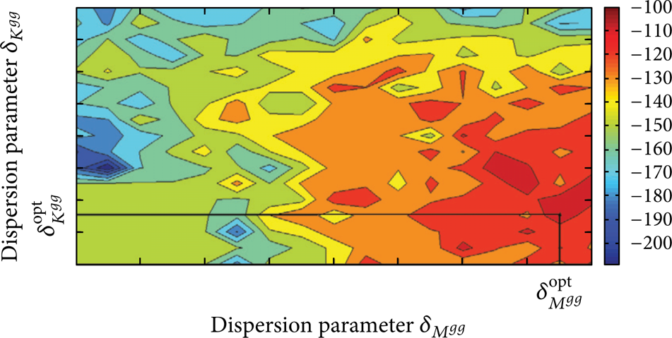
Likelihood function (δ M gg , δ K gg ) → L (δ M gg , δ K gg ). The optimal values are denoted by δ M gg opt and δ K gg opt.

Figure 19:

Confidence region for observation Obs 1: reference stochastic FRF (dark grey region), random frequency response function calculated with the stochastic reduced-order computational model (red region).

Figure 20:

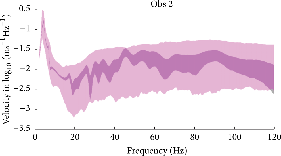
Confidence region for observation Obs 2: reference stochastic FRF (dark grey region), random frequency response function calculated with the stochastic reduced-order computational model (red region).

Figure 21:

Confidence region for observation Obs 3: reference stochastic FRF (dark grey region), random frequency response function calculated with the stochastic reduced-order computational model (red region).

Figure 22:

Confidence region for observation Obs 4: reference stochastic FRF (dark grey region), random frequency response function calculated with the stochastic reduced-order computational model (red region).

5. Conclusion

In this paper, we have applied a recent methodology allowing a reduced-order computational dynamical model to be constructed for the low-frequency domain in which there are simultaneously global and local elastic modes which cannot easily be separated with usual methods. Moreover, we have used the fast marching method which is adapted to complex geometry for constructing the subdomains and the adapted reduced-order computational model. An associated stochastic reduced-order model has then been introduced to take into account uncertainties in the adapted reduced-order model. The results obtained are good with respect to the objectives fixed in this work consisting in constructing a reduced-order model with a very low dimension, which has the capability to predict the frequency responses in the low-frequency range with an sufficient accuracy for a use in the prior project phase.