Sage Journals: Discover world-class research

Abstract

A relation called approximate bisimulation is proposed to achieve behavior and structure optimization for a type of high-level datapath whose data exchange processes are expressed by nonlinear polynomial systems. The high-level datapaths are divided into small blocks with a partitioning method and then represented by polynomial transition systems. A standardized form based on Ritt-Wu's method is developed to represent the equivalence relation for the high-level datapaths. Furthermore, we establish an approximate bisimulation relation within a controllable error range and express the approximation with an error control function, which is processed by Sostools. Meanwhile, the error is controlled through tuning the equivalence restrictions. An example of high-level datapaths demonstrates the efficiency of our method.

1. Introduction

Intelligent transportation systems (ITSs) provide a substantial amount of convenience for daily life. However, with the ever-growing application demands, the scale of ITSs is increasing because ITSs must include an increasing number of features, which will lead us to a difficult situation when designing and verifying the system. With regard to this issue, there is a growing interest in researching how to reduce the scale of the elements in an ITS that involve hardware, software, and other components. In this paper, the research objective is circuit optimization. To achieve the behavior and structure optimization for circuits, the specific data exchange processes must be analyzed. Therefore, we must study circuits at a high level, called high-level datapaths. Complex high-level datapaths typically contain equivalent data exchange processes that are overly complex; worthwhile research on these datapaths considers either how to eliminate the superfluous portion of these processes, known as structure optimization, or how to simplify these processes, known as behavior optimization. In this paper, a novel method is established to address these optimization issues simultaneously for high-level datapaths. Equivalence verification is one of the most commonly used formal methods and is the basis for implementing this method.

There are several equivalent verification tools for circuits, but most of these tools are only suited for circuit verification at a low level, for example, binary decision diagrams (BDDs) [1], word-level decision diagrams (WLDDs) [2], and Taylor expansion diagrams (TEDs) [3]. These tools were all defined on standardized graphs, which have large exponential spaces and time complexities. As a result, verification methods that are based on algebraic methods, such as equivalence verification, have been proposed to solve these problems. Although these methods are very powerful when addressing low-level circuits, they are less suitable for addressing special problems for high-level datapaths. For high-level datapath verification, Smith and Micheli presented a polynomial method for component matching and verification and researched polynomials as allocating components [4, 5]. Moreover, they found a polynomial model for component matching at a high synthesis level [6]. Based on their studies, numerous other research efforts were performed; for instance, the algorithms were proposed to achieve lower costs and minimum timing, driven in high-level data flow synthesis with symbolic algebra [7 –9].

For symbolic algebra, Buchberger demonstrated that useful research must combine a logic method with an algebraic method [10]. In 2006, Zhou also noted that combining these types of methods would be an effective way to verify a system's properties [11]. Based on these ideas, Yang et al. presented a polynomial description and provided a functional equivalence algorithm based on the Groebner bases for one type of high-level datapath, whose data exchange processes are shown by nonlinear polynomial systems. The algorithm was defined from the perspective of common solutions of nonlinear polynomial systems [12]. This work is the first to achieve the functional equivalence of a symbolic method for circuits, and the computing effort is less than that for BMDs or integer linear programming (ILP). However, the optimization is not complete; there is still some potential for improvement. Thus, we provide a more efficient method to achieve the equivalence verification for programs by Ritt-Wu's method in this paper because the characteristic set of a polynomial set achieved by Ritt-Wu's method is unique [13, 14]. Ritt-Wu's method is an algorithm for solving multivariate polynomial equations. It is based on a mathematical concept of characteristic set and powerful for mechanical theorem proving in elementary geometry; then it gives a complete decision process for certain classes of problems.

Equivalence relations require that the behaviors of two high-level datapaths be equivalent, which appears to be impossible using existing technology. For example, consider that we choose two different microwaves to heat bread there are two parameters that we must consider: temperature and time. If both of the ovens can raise the temperature to the same level, then the bread can be heated by the two microwaves. In this case, time is not the critical parameter; the fact that one value is 30.0 s and the other is 29.9 s does not matter. Therefore, these two microwaves can be considered approximately the same. In this case, one of the microwaves, which has a simple behavior and structure, can be used to approximately replace the more complex microwave. This example illustrates that an appropriate approximation can be accepted and provide optimization for different systems without causing a crucial influence. This idea is the key concept that we will utilize to optimize the behavior and structure below and provide a more appropriate relation for high-level datapaths in this paper.

To make this idea come true, an approximate method for a single high-level datapath has already been proposed; this proposal establishes, for the first time, an approximate relation for the corresponding branches in a single datapath [15]. However, this approach does not appear to be a good method for complex circuits that require a large amount of computing effort if we consider the circuits as a whole. Therefore, we must adopt a circuit partitioning method to divide the original datapath into several small blocks. For the circuits, there are already many different partitioning methods based on different demands [16, 17]; considering these methods, a new partitioning method based on an impact factor is proposed in this paper. After being partitioned, an appropriate description of the datapath must be given to research its behavior and structure. A labeled transition system is the basis for achieving this description. Based on this description, an equivalent relation must be proposed to achieve circuit optimization. For the equivalence relation, bisimulation has the best equivalence semantic in process algebra and will be chosen [18]. Bisimulation has been applied to optimize property verifications for different systems, such as hybrid systems and dynamical systems [19 –25]. However, these optimizations still have an issue in that the computing effort could be too large because the original system has not been standardized. We will address this problem here.

In the next section, we will choose nonlinear polynomial sets to represent the data exchange process of a type of high-level datapath in the same way as Yang et al. [12]. To process these sets more conveniently, a datapath partitioning method is proposed to decompose a datapath into several small blocks. To achieve behavior and structure optimization, high-level datapaths are first modeled by polynomial transition systems. Then, a bisimulation relation is proposed. Standardized forms are achieved to determine the equivalence relation for high-level datapaths based on Ritt-Wu's method. In this process, the polynomial sets that correspond to datapaths are changed into triangular sets and provide a space to obtain an approximate relation with their processing nondegeneracy conditions. Subsequently, an error control function is proposed to represent the difference between the datapaths and is processed by a numerical method. Finally, we ensure that our approach obtains circuit optimization by presenting a case study. The proposed method can be used to optimize some circuits within ITS. Our framework is a natural generalization for a type of circuit in ITS that is based on a formal method. For this process, we used Maple and MATLAB as technical tools. The theories of polynomial algebra, polynomial representation of circuits, and algebraic transition systems are the bases of our method, which are mostly available in the literature [12 –14].

2. Partitioning Method and Polynomial Transition System for a High-Level Datapath

In ITS, there are a variety of circuits that can be used to satisfy the variety requirement [26, 27]. When researching the circuits at a high level, their data exchange processes can be expressed by differential semialgebraic systems, differential systems, and polynomial systems, among others. In this paper, we mainly research the circuits for which the data exchange processes can be represented by nonlinear polynomial systems. We have already proposed an approximate method for a single high-level datapath of this type [15], which is suitable only for some simple datapaths. Based on traditional circuit partitioning methods [28 –30], a new partitioning method is introduced in this section to divide a datapath into small blocks for a complex datapath.

2.1. Partitioning Method

Let IF (i, o) be an impact factor for a block in a datapath that sums the number of initial inputs i and final outputs o for this block. After being partitioned, the impact factor of every block is the same or similar. More complex blocks have higher impact factors.

Example 1. Figure 1 presents a datapath in which two inputs, x₁ and x₂, pass through an adder to achieve an intermediate variable v. Then, the output passes through a multiplier that has an additional input of x₃, and then, the output y is obtained.

With a partitioning method, when the impact factor is equal to three, the datapath is divided into two blocks, as shown in Figure 2.

The computing effort and memory usage of these blocks are less than those of the entire datapath. Using previous studies [7, 12], the two blocks in Figure 2 can be described by the following two polynomial sets:

[v - x_{1} - x_{2} = 0], [y - v x_{3} = 0] .

(1)

There is a similarity between a labeled transition system and a high-level datapath after being partitioned. The labeled transition system is composed of limited states and transitions, and every transition represents a relation between inputs and outputs. Because the data exchange processes of high-level datapaths are also described by the polynomial sets to represent the relation between the inputs and outputs, the high-level datapath can be modeled by a labeled transition system, referred to as a polynomial transition system, which is summarized as follows.

Figure 1:

A datapath.

Figure 2:

The datapath after being partitioned.

Definition 2. A polynomial transition system for a high-level datapath is represented by a tuple $〈 Q, L, \to, Q_{0} 〉$ :

a set Q of variables;

a set L of locations;

a set → of transitions; every transition is a tuple $〈 l_{1}, l_{2}, P 〉$ :

l₁ and l₂ are pre- and post-locations of this transition;

P is a first-order assertion represented by a nonlinear polynomial system over Q_I ∪ Q_M ∪ Q_O, where Q_I, Q_M, and Q_O represent the input, middle, and output variables, respectively;

a set Q₀ of initial variables.

The polynomial transition system can be described as a state graph, which contains states and transitions. The entire exchange process between the datapath and polynomial transition system is illustrated in Figure 3.

Figure 3:

The transformation process between a datapath and its polynomial transition system.

In Figure 3, if P₁, P₂, and P₃ have solutions within the same value range and their solutions are equivalent, then the behaviors of these three blocks are identical. In this case, an interesting research topic is determining how to achieve the solutions for the blocks to determine their equivalence relations.

In this paper, k ⊆ Q and k[x] is a ring of polynomials. P ∊ k[x] is a polynomial, and $\overset{—}{x}$ is considered a solution for P or, alternatively, a solution for the polynomial equation P = 0 when $P (\overset{—}{x}) = 0$ . The solutions are all defined in k.

3. Equivalence Determination for High-Level Datapaths Based on Ritt-Wu's Method

For the majority of polynomial sets, the solutions cannot be achieved easily; as a result, it is difficult to determine their equivalence relations. To solve this problem, we use Ritt-Wu's method to standardize the behavior of high-level datapaths first, and we then obtain a standard and unique form to represent equivalence relations without calculating their solutions directly.

By comparing the Groebner basis with Ritt-Wu's approach used in this problem [12], we find that the Groebner basis always results in additional polynomials, which will require a large amount of storage space. In contrast, Ritt-Wu's method allows for simpler and more standardized polynomial sets. At the same time, Ritt-Wu's method is a linear combination of polynomial sets. Its operations are linear, and the degrees are lower as well. Therefore, this method requires less storage space and is more efficient than the Groebner basis.

Before using Ritt-Wu's method to process high-level datapaths, the order of the variables must be defined.

Definition 3. An order relation < is denoted as follows, on S_i ∪ S_m ∪ S_o:

∀ x ∊ S_i, ∀ z ∊ S_m, ∀ y ∊ S_o, then, x < z < y;

∀ x₁, …, x_n ∊ S_i, then, x₁ < · < x_n;

∀ y₁, …, y_n ∊ S_o, then, y₁ < · < y_n;

∀ z₁, …, z_n ∊ S_m

∀ z_i ∊ S_m, ∀ z_k ∊ S_m, ∀ z_j ∊ S_m, z_i, z_k, and z_j represent input, middle, and output variables, respectively; then, z_i < z_j;

∀ m₁, …, m_n ∊ z_i, then, m₁ < · < m_n;

∀ n₁, …, n_n ∊ z_j, then, n₁ < · < n_n,

where DP(S_i, S_m, S_o) is a high-level datapath and S_i, S_m, and S_o represent the input, middle, and output variables, respectively.

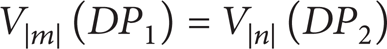
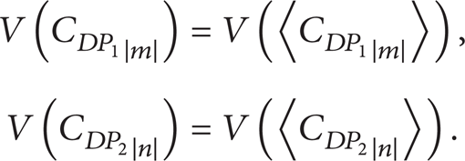
Theorem 4. Two blocks DP₁(x, y, m) and DP₂(x, y, n) are equivalent if

V_{| m |} ({D P}_{1}) = V_{| n |} ({D P}_{2})

(2)

which equals

V ({C_{D P_{1}}}_{| m |}) = V ({C_{D P_{2}}}_{| n |}),

(3)

where all $ini ({C_{D P_{1}}}_{| m |}) = ini ({C_{D P_{2}}}_{| n |}) = 0$ .

Otherwise, it equals

{C_{D P_{1}}}_{| m |} = {C_{D P_{2}}}_{| n |} .

(4)

$V_{| i |} (j)$ represents the solutions for block j after eliminating the middle variables i. ${C_{j}}_{| i |}$ denotes an irreducible characteristic set after eliminating the middle variables i for block j. Here, $ini ({C_{j}}_{| i |})$ is an initial set of ${C_{j}}_{| i |}$ . V(C) is the solution of C.

Proof. It is well known that multivariate polynomial rings over fields are Noetherian; thus, the ideal I can be decomposed into the following:

I = Q_{1} \cap \cdot \cap Q_{m},

(5)

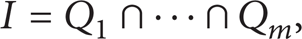
where Q_i is a primary ideal.

Using Ritt-Wu's method, we obtain a variety decomposition: V(P) = ∪ _{i = 1}^eV(P_i).

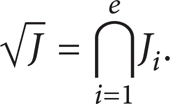
Each P_i defines an unmixed algebraic variety. If V_i = V(P_i), then the above decomposition can be rewritten as

V = V_{1} \cup \cdot \cup V_{e} .

(6)

By irreducible variety decomposition, a decomposition of the radical ideal $\sqrt{J}$ for I is generated by P:

\sqrt{J} = \cap_{i = 1}^{e} J_{i} .

(7)

Thus, $V (\sqrt{J_{D P_{2}}}) = V (\sqrt{J_{D P_{2}}})$ can be represented by $\sqrt{J_{D P_{2}}} = \sqrt{J_{D P_{2}}}$ because the radical ideals cannot be decomposed. Therefore, the two datapaths are equivalent if the solutions of the ideal are the same after eliminating the middle variables.

At the same time,

\begin{matrix} V_{| m |} (C_{D P_{1}}) = V ({〈 C_{D P_{1}} 〉}_{| m |}), \\ V_{| n |} (C_{D P_{2}}) = V ({〈 C_{D P_{2}} 〉}_{| n |}) . \end{matrix}

(8)

Because V(Ideal (P)) = V(P), we have

\begin{matrix} V ({C_{D P_{1}}}_{| m |}) = V (〈 {C_{D P_{1}}}_{| m |} 〉), \\ V ({C_{D P_{2}}}_{| n |}) = V (〈 {C_{D P_{2}}}_{| n |} 〉) . \end{matrix}

(9)

Therefore,

\begin{matrix} V ({C_{D P_{1}}}_{| m |}) = V (〈 {C_{D P_{1}}}_{| m |} 〉) = V ({〈 C_{D P_{1}} 〉}_{| m |}), \\ V ({C_{D P_{2}}}_{| n |}) = V (〈 {C_{D P_{2}}}_{| n |} 〉) = V ({〈 C_{D P_{2}} 〉}_{| n |}) . \end{matrix}

(10)

Thus, if ${C_{D P_{1}}}_{| m |} = {C_{D P_{2}}}_{| n |}$ , then DP₁ and DP₂ are equivalent.

This theorem solves the problem of theoretical determination. It provides us with a unique form to determine equivalent relations for two blocks without calculating their solutions directly and allows our calculation method to be more enriched and strengthened in the process of determining the equivalence relations. With the equivalence determination for blocks, additional blocks can be reduced and complex blocks can be replaced with simpler blocks to achieve structure and behavior optimization. The framework for circuit optimization is illustrated in Figure 4.

Figure 4:

Behavior and structure optimization based on equivalence.

4. Approximate Bisimulation for High-Level Datapaths

After achieving the equivalence relation for the corresponding blocks of a high-level datapath, we next investigate how the equivalence for the entire datapath can be determined.

4.1. The Definition of Approximate Bisimulation

Exact equivalence demands that the solutions of polynomial sets for two datapaths be identical without any error. This constraint appears to be too strict for datapaths in technology because many values of special variables are achieved only by approximation. Thus, in this section, we relax the equivalence restrictions to create a more appropriate relation within a suitable range for all of the datapaths, and we use this relation to achieve behavior and structure optimization. This process is illustrated in Figure 5.

Figure 5:

Behavior and structure optimization based on approximation.

In the process of achieving optimization, bisimulation is applied to establish an approximate equivalence relation for the entire system, as illustrated in Figure 6.

Figure 6:

Nonbisimular.

In this figure, because the dotted part of the left state graph does not have the same trajectory as the right transition graph, they are not equivalent with bisimulation. Bisimulation provides us with the most exact equivalence relation, which can be used to achieve equivalence relations for circuit optimization.

Let $〈 Q_{1}, L_{1}, \to_{1}, {Q_{0}}_{1} 〉$ and $〈 Q_{2}, L_{2}, \to_{2}, {Q_{0}}_{2} 〉$ be polynomial transition systems for two datapaths, DP₁ and DP₂. Here, D is the error, δ is the precision, and → _(D) represents a transition with error D.

Definition 5. A relation S_D ⊆ Q₁ × Q₂ is called an approximate bisimulation, where $D = ∥ P_{1} - P_{2} ∥ \leq δ$ if, for all (x, y) ∊ S_D, P₁ and P₂ have solutions, and the variables of these two systems are the same after substitution:

$\forall x {\overset{P_{1}}{\to}}_{1} x^{'}$ , $\exists y {\overset{P_{2}}{\to}}_{2} y^{'}$ , $\forall x {\overset{P_{1}}{\to}}_{(D)} x^{'}$ such that (x′, y′) ∊ S_D.

$\forall y {\overset{P_{2}}{\to}}_{2} y^{'}$ , $\exists x {\overset{P_{1}}{\to}}_{1} x^{'}$ , $\forall y {\overset{P_{2}}{\to}}_{(D)} y^{'}$ such that (x′, y′) ∊ S_D.

Thus, DP₁ and DP₂ are approximately bisimilar, which means that the solutions of two nonlinear polynomial systems of corresponding blocks are approximately the same for DP₁ and DP₂.

If D > δ, then P₁ and P₂ are not approximately equivalent.

If $D / 2 \leq δ$ , then we can find two polynomial systems C₁′ and C₂′ where there exists

∥ P_{1} - C_{1}^{'} ∥ + ∥ P_{2} - C_{2}^{'} ∥ + ∥ C_{1}^{'} - C_{2}^{'} ∥ \leq δ .

(11)

At the same time, the following hold.

If C₁′ and C₂′ can be changed into two datapaths, then P₁ and P₂ can be replaced with the simpler datapath in C₁′ and C₂′. Therefore, the behavior and structure of DP₁ and DP₂ are approximately optimized.

Otherwise, C₁′ and C₂′ can be used to optimize the safety verification for P₁ and P₂. If C is safe, then

Zero (C) \cap unsafe set =  .

(12)

Because

Zero (P) \subset Zero (C) .

(13)

Thus, P is safe.

If $D / 2 > δ$ , then P₁ and P₂ are not approximately equivalent.

C₁′ and C₂′ are the characteristic sets after ignoring some initials for C₁ and C₂; C₁ and C₂ are the irreducible characteristic sets of P₁ and P₂, respectively.

In this process, the initials of a characteristic set can be considered nondegeneracy conditions because their dimensions are always very low and negligible. For a datapath, an initial is the coefficient of a variable with a high order expressed by a complex unit. If an initial is ignored, then the complex unit is removed to reduce the design costs for the datapath.

With the above analysis, the calculation of approximate bisimulation can be established, which is provided in the next subsection.

4.2. The Calculation Algorithm of Approximate Bisimulation

If the variables of nonlinear polynomial systems of corresponding blocks in a polynomial transition system are the same after substitution, the calculation algorithm of approximate bisimulation for a high-level datapath can be established as follows (see Figure 7).

Figure 7:

Approximate bisimulation for a high-level datapath.

Algorithm 6. The calculation of approximate bisimulation for a high-level datapath.

Input. A high-level datapath whose data exchange processes are represented by nonlinear polynomial systems.

Output. An optimized high-level datapath for the given high-level datapath.

Step 1. Change the high-level datapath into a polynomial transition system. Here, δ is the precision. A group branches according to the bisimulation relation. Suppose that the number of groups is m. Let a counter i = 1.

Step 2. Process the ith group first. Let the precision δ_i in this group belong to

(0, δ - \sum_{e = 1}^{i - 1} δ_{e}) .

(14)

Step 3. Use Ritt-Wu's method to determine the relation of every two branches in this group.

Step 3.1. If the irreducible characteristic sets are identical, then these branches are equivalent. In this case, choose the simplest branch to replace all of the branches and go to Step 5. Otherwise, go to Step 3.2.

Step 3.2. If the errors are not more than δ_i, then these branches are approximately equivalent. In this case, choose an appropriate branch of this group to replace all of the branches and go to Step 5. Otherwise, go to Step 3.3.

Step 3.3. Suppose that the number of branches is a; label them from 1 to a. Let a counter b = 1 and go to Step 4.

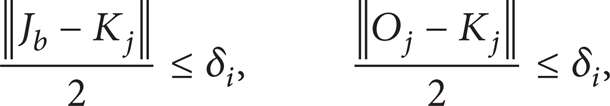
Step 4. Determine the relation between the bth branch and the other branches that form the b + 1th to the ath branch. Let the symbol of the nonlinear polynomial system corresponding to the jth branch be J_j. Let

\begin{matrix} ∊_{b + 1} = ∥ J_{b} - J_{b + 1} ∥, \\ ∊_{b + 2} = ∥ J_{b} - J_{b + 2} ∥, \\ ⋮ \\ ∊_{a} = ∥ J_{b} - J_{a} ∥ . \end{matrix}

(15)

Select J_j except J_b to form a set A when the errors are larger than δ_i. Let the element in A be labeled by K_j. The remaining elements except J_b form the set B. Let the element in B be labeled as O_j. Go to Step 4.1.

Step 4.1. Let U = . The number of elements in A is l. Go to Step 4.2.

Step 4. 2. If there are

\frac{∥ J_{b} - K_{j} ∥}{2} \leq δ_{i}, \frac{∥ O_{j} - K_{j} ∥}{2} \leq δ_{i},

(16)

go to Step 4.2.1. Otherwise, U = A and go to Step 4.5.

Step 4.2.1. Select those elements for which the error of two of the elements is not more than 2δ_i in A to form a new set A′. Merge A′, J_b, and B into a set W. The remaining elements form a set U.

Step 4. 3. If there exist initials in A′, then go to Step 4.3.1. Otherwise, go to Step 4.3.2.

Step 4.3.1. The error caused by the initials of this element is not more than δ_i; then, the characteristic set of this element J_w is used to replace all of the elements in W. Go to Step 4.4. Otherwise, go to Step 4.3.2.

Step 4.3. 2. Use the appropriate element J_w in J_b and O_j to replace and merge all of the elements in J_b and O_j; U = A, and go to Step 4.4.

Step 4. 4. Merge U and J_w to form a new group to be considered as the new ith group. Let the number of branches of this new group be a, b = 2. If a > 2, then go to Step 4; otherwise, go to Step 5.

Step 4. 5. If there exist initials in B, then go to Step 4.5.1. Otherwise, go to Step 4.5.2.

Step 4.5.1. If the error caused by the initials of this element is not more than δ_i, then the characteristic set of the elements in J_w is used to replace all of the elements in J_b and B; go to Step 4.4. Otherwise, go to Step 4.5.2.

Step 4.5. 2. Use J_b to replace J_b and B. Let J_b be J_w, and go to Step 4.4.

Step 5 (i + +). If i ≤ m, then go to Step 2; otherwise, end, and a new nonlinear polynomial transition system is obtained. Thus, the optimized high-level datapath for a given high-level datapath is achieved.

If there are several different high-level datapaths, then we process them with Algorithm 6 to achieve their optimized datapaths. Then, we consider these optimized datapaths to be nondeterministic branches in a new datapath; we determine the equivalent relation for the corresponding branches of this new datapath, choose a simpler branch to replace the complex branches, and achieve the final optimized high-level datapaths.

5. Error Calculation and Error Control Algorithm

This section discusses how to calculate the error, determine whether the error is within an allowable range, and decrease the error if it exceeds the precision requirement.

5.1. Error Control Function

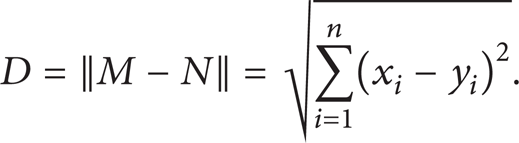
Every point of the original and approximate systems in space can be expressed by a vector. For example, $\vec{O A}$ is the vector of a point in the original system, and $\vec{O B}$ is the vector of a point in the approximate system. The length of $\vec{A B}$ represents the distance between A and B, which also means the difference between them. In this subsection, this difference is called the error. The gradient is a vector field that points in the direction of the greatest increasing rate in the scalar field. Based on this property, we apply a gradient to address the problem of measuring the probability of a change in the trend and the value of the exact error. The specific processes are described below.

Let M(x₁, … x_n) and N(y₁, … y_n) be polynomial systems; then,

G = [\begin{bmatrix} M \\ N \end{bmatrix}] .

(17)

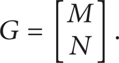
Let the gradient of G be denoted as ∇ G, and let $\vec{O M}$ be a vector for M and $\vec{O N}$ a vector for N. The angle between ∇ G and $\vec{M N}$ is θ.

Positive growth: if θ < 90°, then $(\nabla G) \cdot \vec{M N} \geq 0$ , which indicates that the error is increasing if the gradient is becoming larger. This case is illustrated in Figure 8 (a).

Negative growth: if θ > 90°, then $(\nabla G) \cdot \vec{M N} \leq 0$ , which indicates that the error is decreasing if the gradient is becoming too large. This case is shown in Figure 8 (b).

Figure 8:

Positive and negative growth.

Therefore, the error is reduced when $(\nabla G) \cdot \vec{M N} \leq 0$ . Next, the problem is determining how to apply restrictions to describe the differences and how to set the objective function and solve the optimization problem for two different datapaths.

Let D be an error; then, we can obtain

D = ∥ M - N ∥ = \sqrt{\sum_{i = 1}^{n} {(x_{i} - y_{i})}^{2}} .

(18)

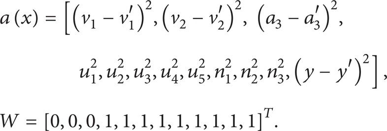
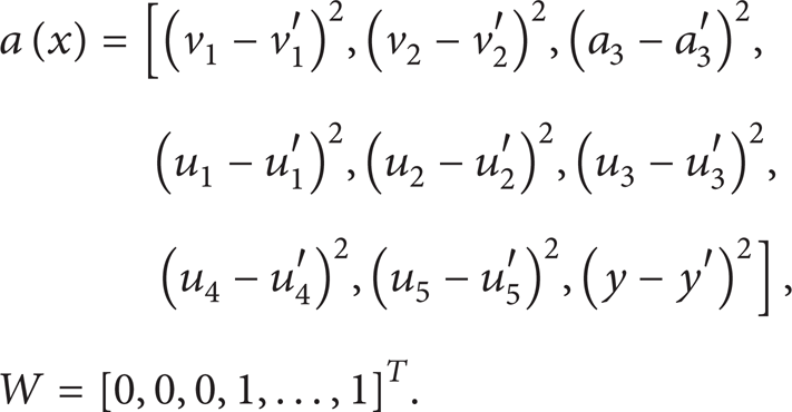
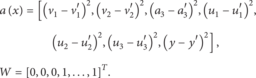
Let a(x) = [(x₁ – y₁)², …, (x_n – y_n)²] be a vector that carries the relational information of the variables between M and N. Compare D with a(x). Suppose that G(x) = K × a(x) is an error control function. Here, ∇ G(X) is the gradient. For all x, y ∊ R, if we expect that D is reduced, then

(\nabla G (x)) \times [\begin{bmatrix} M \\ N \end{bmatrix}] \leq 0 .

(19)

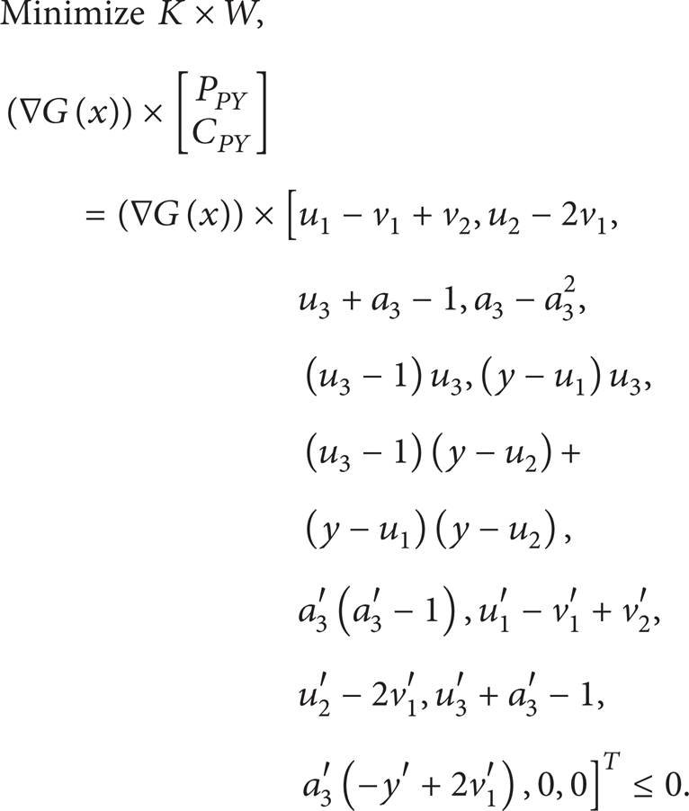
If we also want to minimize the error control function, then we must minimize the value of the coefficient, which is

Minimize K \times W .

(20)

Here, the value of each item in W, when interrelated with the relations between the two systems, is zero or one. For example, if the variables of the two systems are the same, then we only need to determine whether their outputs are identical. Therefore, we obtain a(x) = [(x₁ – y₁)², …, (x_n – y_n)²], W = [0, …, 0, 1]. The values of W and a(x) are unique for every datapath. After achieving the value of K, the error is achieved by

D = \max (\max_{x_{i}} \min_{y_{j}} G (x), \max_{y_{i}} \min_{x_{j}} G (x))

(21)

under the range of values of the variables.

For the nonlinear polynomial systems of datapaths, the number of polynomials may not be equal to the number of variables. To address this problem, we add a new polynomial 0 into the polynomial sets until the numbers of polynomials and variables become identical. The error control function is implemented in MATLAB by the optimization toolbox Sostools.

5.2. Error Control Algorithm

In Section 4, we find that there is a place to achieve an approximate datapath for the original datapath by processing the initials. If the error is large, then the previous ignored initials are readded into a characteristic set to obtain a new approximate characteristic set.

Breadth-first traversal is used in the following algorithm. The first layer and node are labeled by 0.

A description of the symbols used in the algorithm is as follows:

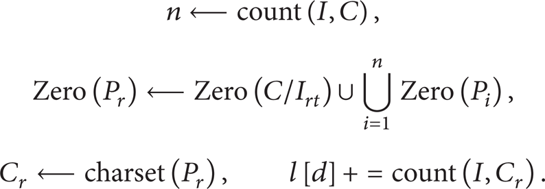
P: a polynomial system;

C: the characteristic set for P;

I: the initial set for C;

D(M, N): an error between two datapaths M and N;

δ: precision;

n ← count (I, C): the number of polynomials in I is n, as counted by a function count;

t ← Crn (r, n): there exist t different choices while adding r initials, t = C_n^r, 1 ≤ r ≤ n – 1;

get (C): obtain one item from C;

getmax (C): obtain one item from C whose dimension is the largest dimension;

set (M, N): merge M and N into one system;

sumresterror (·): sum the remaining error except for the error caused by C;

I_rt: the initials added in the tth time while adding r initials;

k: the subscript of the characteristic sets;

m: the number of polynomials of each characteristic set;

l[d]: the number of initials according to the characteristic sets in the dth layer;

d: the depth of the current layer;

finish: the symbol for the end.

Error control algorithm is as the following.

Algorithm 7. Achieve the approximate polynomial sets for the original polynomial sets and adjust the error within a precision level.

Input. Nonequivalent polynomial sets P₁ and P₂.

Output. Approximate polynomial sets P₁′ and P₂′.

Step 1. Initialize variables: m = 1, k = 1, r = 1, t = 0, and d = 0.

Step 2. Obtain the solution decomposition for P₁ and P₂ with Ritt-Wu's method:

\begin{matrix} Zero (P_{1}) = Zero (C_{1} / I) \cup \overset{m}{\underset{i = 1}{\cup}} Zero (P_{i}), \\ Zero (P_{2}) = Zero (C_{2} / I) \cup \overset{n}{\underset{j = 1}{\cup}} Zero (P_{j}), \end{matrix}

(22)

where m = count (I, C₁) and n = count (I, C₂).

Let P = set (P₁, P₂) and S = set (C₁, C₂).

Step 3. Ignore all of the initials for C₁ and C₂. Obtain D₁ = D(P₁, C₁), D₂ = D(P₂, C₂), and D = D(C₁, C₂).

Step 4. If D + D₁ + D₂ < δ, C₁ ≅ C₂. Let P₁′ = C₁, P₂′ = C₂. Go to Step 4.1. Otherwise, go to Step 4.2.

Step 4.1. If C₁ and C₂ cannot be changed into datapaths, then the new approximate polynomial sets cannot be achieved; end. Otherwise, the simpler choice between C₁ and C₂ is chosen to replace P₁ and P₂; end.

Step 4.2. If S is an empty set, then C₁ ≇ C₂, P₁ ≇ P₂, and error = ∞; end. Otherwise, go to Step 5.

Step 5. Let

\begin{matrix} C ⟵ getmax (S), \\ Terror ⟵ sumresterror (C), \\ P ⟵ get (C) . \end{matrix}

(23)

Step 6. If C is contradictory, then go to Step 9. Otherwise, go to Step 7.

Step 7. If finish = true, then go to Step 10. Otherwise,

\begin{matrix} n ⟵ count (I, C), \\ Zero (P_{r}) ⟵ Zero (C / I_{r t}) \cup \overset{n}{\underset{i = 1}{\cup}} Zero (P_{i}), \\ C_{r} ⟵ charset (P_{r}), l [d] + = count (I, C_{r}) . \end{matrix}

(24)

Go to Step 8.

Step 8. If D(P, P_r) + Terror < δ, then finish ← true and go to Step 7. Otherwise, r ← r + 1, t ← Crn (r, n), and go to Step 8.1.

Step 8.1. If r > n – 1, then go to Step 9. Otherwise, go to Step 7.

Step 9 (k + +). If k > m, then go to Step 9.1. Otherwise, go to Step 9.2.

Step 9.1. If l[d] = 0 and P₁ ≇ P₂, end. Otherwise, m = l[d], C ← C_k, d ← d + 1, and l[d] = 0, and go to Step 6.

Step 9.2. C ← C_k; go to Step 6.

Step 10. If P₁′ and P₂′ can be changed into the datapaths P₁′ ≅ P₂′, then end. Otherwise, approximate datapaths cannot be achieved; end.

With this algorithm, the error can be controlled by readding the ignored initials. If the final error is still larger than the precision, then there is no approximate relation based on our method.

In the process of this algorithm, there is a critical step that requires special attention. The currently added initials may not be able to achieve our desired goal, which means that they cannot reduce the error when D > δ. This problem is caused by the relationship among the zeros of the polynomial sets, the characteristic sets, and their initials. Therefore, we must analyze the relationship so that we can choose the appropriate initials to decrease the error as soon as possible.

5.3. Choose the Appropriate Initials

Choosing the appropriate initials will allow us to reduce the computing efforts. With the relationship among the solutions of the polynomial sets, the characteristic sets, and their initials, there are three different types of functions for the added initials. Next, let P be a polynomial set for a block of a datapath. C is a characteristic set for P, and I = [I₁, …, I_r] is the initial set for C. According to Ritt-Wu's decomposition,

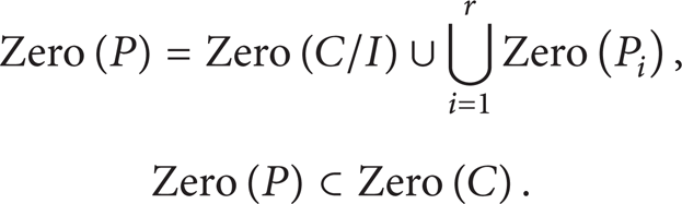
\begin{matrix} Zero (P) = Zero (C / I) \cup \cup_{i = 1}^{r} Zero (P_{i}), \\ Zero (P) \subset Zero (C) . \end{matrix}

(25)

Theorem 8. The function of added initials has three cases. The value ranges of the solutions are represented by circles.

C and I have no intersection. This type of initial cannot reduce the error. The solution relationship of P, C, and I is shown in Figure 9 (a).

C and I have an intersection, and I ⊂ C. The function of these initials can be divided into two cases, and the solution relationship of P, C, and I is shown in Figure 9 (b).

If I_i ⊂ P ∩ I, then these initials cannot reduce the error.

If I_i ⊄ P ∩ I, then these initials can reduce the error.

C and I have an intersection, but if ∃ I_i ∩ C = , the function of these initials has two different cases, and the solution relationship of P, C, and I is shown in Figure 9 (c).

If I_i ⊂ P ∩ I, then these initials cannot reduce the error by adding them.

If I_i ⊄ P ∩ I, then there are two cases for the effect of the initials.

If I_i ⊄ C, then these initials cannot reduce the error.

If I_i ⊂ C, then these initials reduce the error by adding them.

Figure 9:

Solution relationship.

Using the above analysis, we can select the most appropriate initial to control the error as soon as possible.

6. Example Verification and Main Results

Let us consider two high-level datapaths DP₁ and DP₂ in the ITS shown in Figures 10 and 11, where δ = 5e – 15. In these figures, DP₁ and DP₂ have complex units. The datapath partitioning method is applied to reduce the computing effort. The impact factor equals four, and then, DP₁ is divided into four parts and DP₂ is divided into two parts, as shown in Figures 12 and 13.

Figure 10:

DP₁.

Figure 11:

DP₂.

Figure 12:

DP₁ after being partitioned.

Figure 13:

DP₂ after being partitioned.

Blocks 1 and 3 for DP₁ and DP₂ are identical. Therefore, we only demand to determine the relationship among blocks 2, 3, and 4 for DP₁. If these blocks are equivalent or approximately equivalent, then DP₁ and DP₂ are the bisimulation equivalent or approximate equivalent and we can replace DP₁ with DP₂.

The polynomial representations for DP₁ are as follows:

Block 2 PB:

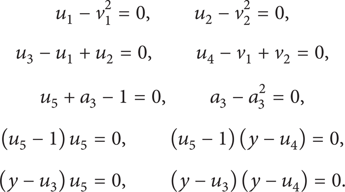
\begin{matrix} u_{1} - v_{1}^{2} = 0, u_{2} - v_{2}^{2} = 0, \\ u_{3} - u_{1} + u_{2} = 0, u_{4} - v_{1} + v_{2} = 0, \\ u_{5} + a_{3} - 1 = 0, a_{3} - a_{3}^{2} = 0, \\ (u_{5} - 1) u_{5} = 0, (u_{5} - 1) (y - u_{4}) = 0, \\ (y - u_{3}) u_{5} = 0, (y - u_{3}) (y - u_{4}) = 0 . \end{matrix}

(26)

Block 3 PY:

\begin{matrix} n_{1} - v_{1} + v_{2} = 0, n_{2} - 2 v_{1} = 0, \\ n_{3} + a_{3} - 1 = 0, a_{3} - a_{3}^{2} = 0, \\ (n_{3} - 1) n_{3} = 0, (y - n_{1}) n_{3} = 0, \\ (n_{3} - 1) (y - n_{2}) = 0, (y - n_{1}) (y - n_{2}) = 0 . \end{matrix}

(27)

Block 4 PG:

\begin{matrix} m_{1} - v_{1} + v_{2} = 0, m_{2} - v_{1} - v_{2} = 0, \\ m_{3} - m_{1} m_{2} = 0, m_{4} + a_{3} - 1 = 0, \\ (a_{3} - 1) a_{3} = 0, (m_{4} - 1) m_{4} = 0, \\ (m_{4} - 1) (y - m_{1}) = 0, (y - m_{3}) m_{4} = 0, \\ (y - m_{3}) (y - m_{1}) = 0 . \end{matrix}

(28)

We compute the characteristic sets for these blocks by Ritt-Wu's method. The results are as follows after removing the middle variables:

\begin{matrix} {C_{P B}}_{| u |} = {C_{P G}}_{| m |} = [(a_{3} - 1) a_{3}, a_{3} (- y + v_{1} - v_{2})], \\ {C_{P B}}_{| u |} = [(a_{3} - 1) a_{3}, a_{3} (- y + v_{1} - v_{2})] \\ \neq {C_{P Y}}_{| n |} = [(a_{3} - 1) a_{3}, a_{3} (- y + 2 v_{1})] . \end{matrix}

(29)

Thus, block 2 is equivalent to block 4.

However, for blocks 2 and 3, we must establish an error control function, check the value of the error, and determine whether the error is within the expected precision. The entire process is described below.

Let the variables ∊ [0, 1], and let the symbols of the variables {x, y, a} of the second system be changed to {x′, y′, a′} by a substitution rule to facilitate the calculation.

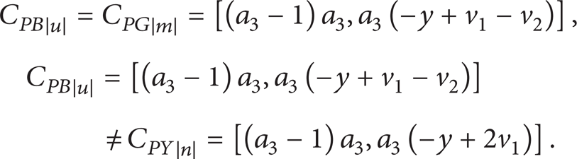
For P_PB and P_PY,

\begin{matrix} a (x) = [{(v_{1} - v_{1}^{'})}^{2}, {(v_{2} - v_{2}^{'})}^{2}, {(a_{3} - a_{3}^{'})}^{2}, u_{1}^{2}, u_{2}^{2}, u_{3}^{2}, u_{4}^{2}, u_{5}^{2}, n_{1}^{2}, n_{2}^{2}, n_{3}^{2}, {(y - y^{'})}^{2}], \\ W = {[0,0, 0,1, 1,1, 1,1, 1,1, 1,1]}^{T} . \end{matrix}

(30)

Then,

\begin{matrix} Minimize K \times W, \\ (\nabla G (x)) \times [\begin{bmatrix} P_{P B} \\ P_{P Y} \end{bmatrix}] \\ = (\nabla G (x)) \times [u_{1} - v_{1}^{2}, u_{2} - v_{2}^{2}, u_{3} - u_{1} + u_{2}, \\ u_{4} - v_{1} + v_{2}, u_{5} + a_{3} - 1, \\ a_{3} - a_{3}^{2}, (u_{5} - 1) u_{5}, \\ (u_{5} - 1) (y - u_{4}), \\ (y - u_{3}) u_{5} + (y - u_{3}) (y - u_{4}), \\ n_{1} - v_{1}^{'} + v_{2}^{'}, n_{2} - 2 v_{1}^{'}, \\ n_{3} + a_{3}^{'} - 1, a_{3}^{'} - a_{3}^{' 2}, \\ (n_{3} - 1) n_{3}, (y^{'} - n_{1}) (n_{3} - 1), \\ (n_{3} - 1) (y^{'} - n_{2}) \\ {+ (y^{'} - n_{1}) (y^{'} - n_{2})]}^{T} \leq 0 . \end{matrix}

(31)

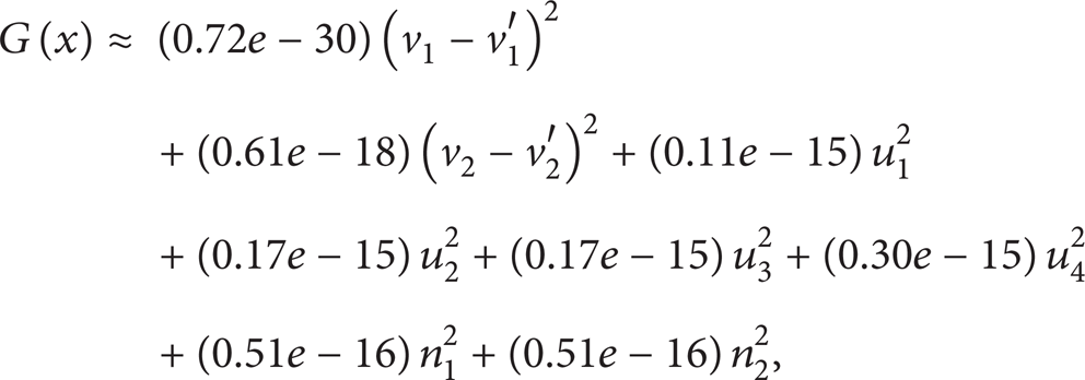
After computation, the error control function is

G (x) \approx (0.85 e - 15) u_{1}^{2} + (0.85 e - 15) u_{2}^{2} + (0.85 e - 12) u_{3}^{2} + (0.18 e - 15) u_{4}^{2} + (0.18 e - 15) u_{5}^{2} + (0.65 e - 15) {(y - y^{'})}^{2} + (0.85 e - 15) n_{1}^{2} + (0.85 e - 15) n_{2}^{2} + 0.85 e - 15 n_{3}^{2},

(32)

D = max(G(x)) ≈ 6.1e – 15 > 5e – 15; thus, P_PB and P_PY are not approximate.

For C_PB and C_PY,

\begin{matrix} a (x) = [{(v_{1} - v_{1}^{'})}^{2}, {(v_{2} - v_{2}^{'})}^{2}, {(a_{3} - a_{3}^{'})}^{2}, u_{1}^{2}, u_{2}^{2}, u_{3}^{2}, u_{4}^{2}, u_{5}^{2}, n_{1}^{2}, n_{2}^{2}, n_{3}^{2}, {(y - y^{'})}^{2}], \\ W = {[0,0, 0,1, 1,1, 1,1, 1,1, 1,1]}^{T} . \end{matrix}

(33)

Then,

\begin{matrix} Minimize K \times W, \\ (\nabla G (x)) \times [\begin{bmatrix} C_{P B} \\ C_{P Y} \end{bmatrix}] \\ = (\nabla G (x)) \times [(a_{3} - 1) a_{3}, u_{1} - v_{1}^{2}, u {}_{2} - v_{2}^{2}, \\ u_{3} - v_{1}^{2} + v_{2}^{2}, u_{4} - v_{1} + v_{2}, \\ u_{5} + a_{3} - 1, a_{3} (- y + v_{1} - v_{2}), \\ 0,0, a_{3}^{'} (a_{3}^{'} - 1), n_{1}^{'} - v_{1}^{'} + v_{2}^{'}, \\ n_{2}^{'} - 2 v_{1}^{'}, n_{3}^{'} + a_{3}^{'} - 1, \\ {a_{3}^{'} (- y^{'} + 2 v_{1}^{'}), 0,0]}^{T} \leq 0 . \end{matrix}

(34)

The error control function is

G (x) \approx (0.72 e - 30) {(v_{1} - v_{1}^{'})}^{2} + (0.61 e - 18) {(v_{2} - v_{2}^{'})}^{2} + (0.11 e - 15) u_{1}^{2} + (0.17 e - 15) u_{2}^{2} + (0.17 e - 15) u_{3}^{2} + (0.30 e - 15) u_{4}^{2} + (0.51 e - 16) n_{1}^{2} + (0.51 e - 16) n_{2}^{2},

(35)

D₁ = max(G(x)) ≈ 8.63e – 16.

For P_PB and C_PB,

\begin{matrix} a (x) = [{(v_{1} - v_{1}^{'})}^{2}, {(v_{2} - v_{2}^{'})}^{2}, {(a_{3} - a_{3}^{'})}^{2}, {(u_{1} - u_{1}^{'})}^{2}, {(u_{2} - u_{2}^{'})}^{2}, {(u_{3} - u_{3}^{'})}^{2}, {(u_{4} - u_{4}^{'})}^{2}, {(u_{5} - u_{5}^{'})}^{2}, {(y - y^{'})}^{2}], \\ W = {[0,0, 0,1, \dots, 1]}^{T} . \end{matrix}

(36)

Then,

\begin{matrix} Minimize K \times W, \\ (\nabla G (x)) \times [\begin{bmatrix} P_{P B} \\ C_{P B} \end{bmatrix}] \\ = (\nabla G (x)) \times [u_{1} - v_{1}^{2}, u_{2} - v_{2}^{2}, u_{3} - u_{1} + u_{2}, \\ u_{4} - v_{1} + v_{2}, u_{5} + a_{3} - 1, \\ a_{3} - a_{3}^{2}, (u_{5} - 1) u_{5}, \\ (u_{5} - 1) (y - u_{4}), \\ (y - u_{3}) u_{5} + (y - u_{3}) (y - u_{4}), \\ (a_{3}^{'} - 1) a_{3}^{'}, u_{1}^{'} - v_{1}^{' 2}, \\ u_{2}^{'} - v_{2}^{' 2}, u_{3}^{'} - v_{1}^{' 2} + v_{2}^{' 2}, \\ u_{4}^{'} - v_{1}^{'} + v_{2}^{'}, u_{5}^{'} + a_{3}^{'} - 1, \\ {a_{3}^{'} (- y^{'} + v_{1}^{'} - v_{2}^{'}), 0,0]}^{T} \leq 0 . \end{matrix}

(37)

The error control function is

\begin{matrix} G (x) \approx - (0.68 e - 9) {(u_{5} - u_{5}^{'})}^{2} \\ - (0.68 e - 9) {(u_{4} - u_{4}^{'})}^{2} - (0.68 e - 9) {(u_{3} - u_{3}^{'})}^{2} \\ - (0.68 e - 9) {(u_{2} - u_{2}^{'})}^{2} \\ - (0.68 e - 9) {(u_{1} - u_{1}^{'})}^{2} - (0.68 e - 9) {(y - y^{'})}^{2}, \end{matrix}

(38)

D₂ = max(G(x)) = 0.

For P_PY and C_PY,

\begin{matrix} a (x) = [{(v_{1} - v_{1}^{'})}^{2}, {(v_{2} - v_{2}^{'})}^{2}, {(a_{3} - a_{3}^{'})}^{2}, {(u_{1} - u_{1}^{'})}^{2}, {(u_{2} - u_{2}^{'})}^{2}, {(u_{3} - u_{3}^{'})}^{2}, {(y - y^{'})}^{2}], \\ W = {[0,0, 0,1, \dots, 1]}^{T} . \end{matrix}

(39)

Then,

\begin{matrix} Minimize K \times W, \\ (\nabla G (x)) \times [\begin{bmatrix} P_{P Y} \\ C_{P Y} \end{bmatrix}] \\ = (\nabla G (x)) \times [u_{1} - v_{1} + v_{2}, u_{2} - 2 v_{1}, \\ u_{3} + a_{3} - 1, a_{3} - a_{3}^{2}, \\ (u_{3} - 1) u_{3}, (y - u_{1}) u_{3}, \\ (u_{3} - 1) (y - u_{2}) + (y - u_{1}) (y - u_{2}), \\ a_{3}^{'} (a_{3}^{'} - 1), u_{1}^{'} - v_{1}^{'} + v_{2}^{'}, \\ u_{2}^{'} - 2 v_{1}^{'}, u_{3}^{'} + a_{3}^{'} - 1, \\ {a_{3}^{'} (- y^{'} + 2 v_{1}^{'}), 0,0]}^{T} \leq 0 . \end{matrix}

(40)

The error control function is

G (x) \approx (0.23 e - 14) (v_{1} - v_{1}^{'}) + (0.10 e - 15) (v_{2} - v_{2}^{'}),

(41)

D₃ = max(G(x)) ≈ 2.42e – 15. D = D₁ + D₂ + D₃ ≈ 3.28e – 15 < 5e – 15; thus, C_PB and C_PY are approximate.

Therefore, we achieve two approximate systems C_PB and C_PY for PB and PY, respectively.

In Yang's paper, the equivalence verification for high-level datapaths is determined using the Groebner basis. The number of polynomials and the computing effort are given in Figure 14 when processing blocks 2, 3, and 4 for DP₁ using the Groebner basis and the Ritt-Wu method.

Figure 14:

Results.

Figure 14 illustrates that less computing effort is required with fewer polynomials. Ritt-Wu's method is better than the Groebner basis for the equivalence verification of datapaths. Because the Groebner basis is better than BMDs and ILP [12], our method is the best method among the methods considered for the equivalence verification process for circuits.

Furthermore, four results are achieved:

For P_PB and C_PB and P_PY and C_PY, their exact errors caused by ignoring initials are 0 and 2.42e – 15, respectively. Thus, our method is reasonable in that we consider initials as nondegeneracy conditions because their effects are always very small.

According to Ritt-Wu's method, C_PB, C_PY, and C_PG are triangular sets; these sets are more standardized than P_PB, P_PY, and P_PG. In this case, our method costs less in terms of computing effort when processing property verification is based on state because the systems are standardized first by a symbolic method.

The exact error can be calculated through the error control function. For example, when D(P_PB, P_PY) ≈ 6.1e – 15 > δ, we get the approximate systems C_PB and C_PY for P_PB and P_PY with ignoring the initials of characteristic sets. The final error is 3.28e – 15, which meets the precision requirement. C_PB and C_PY cannot be changed into new datapaths, but they can be applied to optimize the property verification of circuits in the future, such as safety verification, because C is more standardized and its solutions is more than P.

With approximate bisimulation, block 4 can be removed in DP₁′; thus, circuit optimization is achieved. Because the numbers of states and blocks are all reduced, the property verification based on the states can be optimized for the circuits.

7. Conclusion

In this paper, a new partitioning method is established to divide a type of high-level datapath in ITS into small blocks to reduce the computing efforts. Next, the datapaths are modeled by polynomial transition systems to provide a framework to research their behavior and structure. Then, an approximate bisimulation based on symbolic-numeric computation is proposed, which is used to obtain behavior and structure optimization for the datapaths. The result of the introduced example illustrates that the computing efforts caused by our new method are less than those of the Groebner basis, BMDs, and ILP in the equivalence verification process for circuits.

However, additional research on this topic is still required. Because some approximate polynomial systems cannot be turned into new datapaths, for example, C_PB and C_PY, we will investigate the readabilities for these approximate systems. At the same time, because the characteristic sets are more standardized than the original polynomial sets, they can be used to optimize the property verification for the circuits in ITS; this goal is briefly introduced in Section 4 and will be implemented in the future.

Footnotes

Acknowledgments

This work was supported by the National Natural Science Foundation of China under Grant no. 11371003, the Natural Science Foundation of Guangxi under Grants nos. 2011GXNSFA018154 and 2012GXNSFGA060003, the Science and Technology Foundation of Guangxi under Grant no. 10169-1, and the Scientific Research Project no. 201012MS274 from Guangxi Education Department.

References

Bryant

R. E.

, “Graph-based algorithms for boolean function manipulation,” IEEE Transactions on Computers, vol. C–35, no. 8, pp. 677–691, 1986.

Bryant

R. E.

and Chen

Y.-A.

, “Verification of arithmetic circuits with binary moment diagrams,” in Proceedings of the 32nd Design Automation Conference, pp. 535–541, June 1995.

Ciesielski

Kalla

, and Askar

, “Taylor expansion diagrams: a canonical representation for verification of data flow designs,” IEEE Transactions on Computers, vol. 55, no. 9, pp. 1188–1201, 2006.

Smith

and De Micheli

, “Polynomial methods for component matching and verification,” in Proceedings of the IEEE/ACM International Conference on Computer-Aided Design (ICCAD '98), pp. 678–685, November 1998.

James

and Giovanni

D. M.

, “Polynomial methods for allocating complex components,” in Proceedings of the Conference on Design, Automation and Test in Europe, pp. 217–222, 1999.

Smith

and De Micheli

, “Polynomial circuit models for component matching in high-level synthesis,” IEEE Transactions on Very Large Scale Integration (VLSI) Systems, vol. 9, no. 6, pp. 783–800, 2001.

Peymandoust

and De Micheli

, “Using symbolic algebra in algorithmic level DSP synthesis,” in Proceedings of the 38th Design Automation Conference, pp. 277–282, June 2001.

Giovanni

D. M.

and Armita

, “Symbolic algebra and timing driven data-flow synthesis,” in Proceedings of the IEEE/ACM International Conference on Computer Aided Design (ICCAD '01), pp. 300–305, San Jose, Calif, USA, 2001.

Peymandoust

and De Micheli

, “Application of symbolic computer algebra in high-level data-flow synthesis,” IEEE Transactions on Computer-Aided Design of Integrated Circuits and Systems, vol. 22, no. 9, pp. 1154–1165, 2003.

10.

Buchberger

, “A view on the future of symbolic computation,” in Proceedings of the International Symposium on Symbolic and Algebraic Computation (ISSAC '05), p. 1, ACM Press, July 2005.

11.

Zhou

C. C.

, “Program verification through computer algebra,” in Formal Methods and Software Engineering, Lecture Notes in Computer Science, p. 4360, 2006.

12.

Yang

Guangsheng

, and Shao

, “A symbolic methodology for formal verification of high-level data-flow synthesis,” in Proceedings of the 9th International Conference on Solid-State and Integrated-Circuit Technology (ICSICT '08), pp. 2353–2356, Beijing, China, October 2008.

13.

Chou

S. C.

and Gao

X. S.

, “Ritt-Wu's decomposition algorithm and geometry theorem proving,” in Proceedings of the 10th International Conference on Automated Deduction, vol. 449 of Lecture Notes in Computer Science, pp. 207–220, 1990.

14.

Wang

, “An elimination method for polynomial systems,” Journal of Symbolic Computation, vol. 16, no. 2, pp. 83–114, 1993.

15.

Deng

J. Z.

, and Zhou

, “Approximate equivalence and optimization for high-level datapath,” Journal of Information and Computational Science, vol. 8, no. 16, pp. 4131–4142, 2011.

16.

Girard

Guller

, and Landraul

, “Low power BIST design by hypergraph partitioning: methodology and architectures,” in Proceedings of the International Test Conference, pp. 652–661, 2000.

17.

Banos

Gil

Montoya

M. G.

, and Ortega

, “A parallel evolutionary algorithm for circuit partitioning,” in Proceedings of the 11h Euromicro Conference on Parallel, Distributed and Network Based Processing, pp. 365–371, 2003.

18.

Van Glabbeek

R. J.

, “The linear time-branching time spectrum,” in Proceedings of the 4th International Conference on Concurrency Theory (CONCUR '93), vol. 458 of Lecture Notes in Computer Science, pp. 278–297, Hildesheim, Germany, 1990.

19.

Pappas

G. J.

, “Bisimilar linear systems,” Automatica, vol. 39, no. 12, pp. 2035–2047, 2003.

20.

van der Schaft

A. J.

, “Equivalence of dynamical systems by bisimulation,” IEEE Transactions on Automatic Control, vol. 49, no. 12, pp. 2160–2172, 2004.

21.

Girard

and Pappas

G. J.

, “Approximation metrics for discrete and continuous systems,” IEEE Transactions on Automatic Control, vol. 52, no. 5, pp. 782–798, 2007.

22.

Girard

and Pappas

G. J.

, “Approximate bisimulations for nonlinear dynamical systems,” in Proceedings of the 44th IEEE Conference on Decision and Control, and the European Control Conference (CDC-ECC '05), pp. 684–689, December 2005.

23.

Girard

and Pappas

G. J.

, “Approximate bisimulation relations for constrained linear systems,” Automatica, vol. 43, no. 8, pp. 1307–1317, 2007.

24.

Julius

A. A.

, “Approximate abstraction of stochastic hybrid automata,” in Hybrid Systems: Computation and Control, vol. 3927 of Lecture Notes in Computer Science, pp. 318–332, 2006.

25.

Van der Schaft

, “Bisimulation of dynamical systems,” in Hybrid Systems: Computation and Control, vol. 2993 of Lecture Notes in Computer Science, pp. 555–569, 2004.

26.

Wang

Guo

Bubb

, and Ikeuchi

, “Numerical simulation and analysis procedure for model-based digital driving dependability in intelligent transport system,” KSCE Journal of Civil Engineering, vol. 15, no. 5, pp. 891–898, 2011.

27.

Wang

W. H.

Cao

Ikeuchi

, and Bubb

, “Reliability and safety analysis methodology for identification of drivers' erroneous actions,” International Journal of Automotive Technology, vol. 11, no. 6, pp. 873–881, 2010.

28.

Mak

W.-K.

and Wong

D. F.

, “Fast hypergraph min-cut algorithm for circuit partitioning,” Integration, the VLSI Journal, vol. 30, no. 1, pp. 1–11, 2000.

29.

Coe

Areibi

, and Moussa

, “A hardware Memetic accelerator for VLSI circuit partitioning,” Computers and Electrical Engineering, vol. 33, no. 4, pp. 233–248, 2007.

30.

Bultan

and Aykanat

, “Circuit partitioning using mean field annealing,” Neurocomputing, vol. 8, no. 2, pp. 171–194, 1995.

Approximate Bisimulation for High-Level Datapaths in Intelligent Transportation Systems

Abstract

1. Introduction

2. Partitioning Method and Polynomial Transition System for a High-Level Datapath

2.1. Partitioning Method

3. Equivalence Determination for High-Level Datapaths Based on Ritt-Wu's Method

4. Approximate Bisimulation for High-Level Datapaths

4.1. The Definition of Approximate Bisimulation

4.2. The Calculation Algorithm of Approximate Bisimulation

5. Error Calculation and Error Control Algorithm

5.1. Error Control Function

5.2. Error Control Algorithm

5.3. Choose the Appropriate Initials

6. Example Verification and Main Results

7. Conclusion

Footnotes

Acknowledgments

References