Achieving Network Localizability in Nonlocalizable WSN with Moving Passive Event

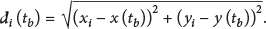
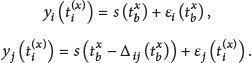
Abstract

Localization is an essential service in most of the wireless sensor network (WSN) applications. This paper focuses on utilizing the moving passive event to achieve the network localizability in an initially nonlocalizable network. The hybrid TDOA and distance measurement is firstly used in the network localizability. We propose the sufficient conditions in terms of node localizability and network localizability, respectively. Besides, a more promising TDOA estimation approach, which is approximately synchronization-free, is proposed to well support our localization approach. We design a corresponding algorithm in distributed manner for the implementation of our approach. Compared with the current works, our approach requires no extra hardware cost and any adjustment of the current topology of the network and hence is more feasible in practice. We evaluate the performance of our approach via extensive simulations on a one-thousand-node network. Simulation results show that our TDOA estimation approach achieves the accuracy of 0.1 milliseconds. More than 90% nodes can be localized within 0.04r, where r denotes the ranging radius of a sensor.

1. Introduction

Localization [1] is one of the most significant research issues in the low-power wireless sensor networks (WSN). Due to the unavailability and the large energy consumption of the GPS receiver, many research efforts focus on the cooperative localization [2, 3]. In such a setting, some special nodes, called beacons, know their global locations and the rest nodes determine their locations by measuring the distances to their neighbors.

Despite those innovative efforts, a WSN may still not be entirely localized. Such a network is called nonlocalizable network. Previous study [4] indicates that, unless a network is dense, it is unlikely that all of the nodes in the network can be uniquely localized. A WSN, however, is usually not excessively dense because the topology control mechanism is used to alleviate collision and interference in practice. Moreover, the randomness in the deployment may also influence the localizability of a WSN. For example, the sensors may be deployed rapidly and randomly to the field through a rocket or UAV in military applications. As such, the topology of the network is difficult to be predicated or accurately controlled, due to the influence of many factors such as wind and terrain. Figure 1 shows an example of the nonlocalizable network, where the edges denote the measurable distances between the corresponding nodes. The sensors are released randomly to the two sides of a road. Obviously, the network is not entirely localizable since it is not global rigid. We also find evidences via observations from the Ocean Sense [5] and GreenOrbs [6] projects. The networks in the two real applications are not entirely localizable in their initial deployments.

Figure 1

An example of nonlocalizable network.

The nonlocalizable network leads to the research on the localizability problem. Graph rigidity theory [4, 7, 8] is utilized to differ the localizable part and nonlocalizable part of a WSN. Localizing the nonlocalizable part is a challenging issue. Obviously, neither manual calibrating the location of each sensor nor equipping each sensor with the global positioning system (GPS) receiver or the other equivalent devices is practical for a large-scale wireless sensor network. An alternative approach is to deploy additional nodes or beacons to create abundant internode distance constraints, so as to enhance the level of network localizability. Such kind of approaches, however, is difficult to find and implement an efficient redeployment plan without the locations of all nodes.

The current efforts to localize the nonlocalizable part of the WSN fall into one of the three categories: (1) the probabilistic based approaches [4, 9, 10] use different probabilistic models to infer the location of each node via extensive observations, but lack of accuracy and incur large computational overhead; (2) mobile assisted approaches [11–13] use some controllable mobile nodes to provide thorough information for localization, but require extra expensive hardware (e.g., a mobile robot) and incur much more adjustment delay and controlling overheads; (3) network adjustment approaches [14–16] increase the ranging capability of some sensor nodes to provide additional distance constraints and hence achieve the network localizability, but require to adequately augment numerous sensors adaptively and incurs more energy consumption. Therefore, it is crucial to propose a high-accuracy, low-cost, and scalable localization approach to achieve the network localizability in a nonlocalizable WSN.

This paper focuses on how to use the hybrid distance and time difference of arrival (TDOA) measurement to achieve network localizability. Our approach is based on a simple but interesting finding that the TDOA measurement can provide additional distance constrains together with the distance measurement. When a passive event that emits a certain kind of signal, for example, vehicle, is moving through the sensor filed, the thorough TDOA observations between all one-hop neighbors can be achieved. As such, given the time-varying locations of the event, an initially nonlocalizable node can be localized if it has at least one localizable one-hop neighbor. Actually, the trajectory of the event can be determined by the localizable part in a partially localizable network with current target tracking approaches [17–20] and hence is assumed to be known as a priori.

The contributions of this paper are summarized as follows.

First of all, we utilize the TDOA observation to obtain additional distance constrains and achieve the network localizability. We propose the sufficient condition in terms of node localizability and network localizability when a passive event is passing through the sensor field. The localizability condition with moving passive event is relaxed to that any connected network contains at least one beacon. It is much easier to achieve in practice. To the best of our knowledge, we are the first to utilize the passive event to achieve the localizability in an initial nonlocalizable network.

Additionally, we propose an approximately synchronization-free approach to estimate the TDOA of the signal emitted by a moving event for one-hop neighbors. The TDOA is estimated by generalized cross correlating their sampled signals in frequency domain. Simulation results show that its accuracy can achieve 0.1 milliseconds or better.

Last but not least, we design a localization algorithm in distributed manner. To alleviate the cumulative error during the process of localization, the credit of each localized sensor is utilized to select more reliable reference nodes. Simulation results show that, for a sparse network whose average node degree is 4.92, the average localization error is below 7 percent of the measuring range of a sensor. As the density of the network grows, such an error is about 2 percent of the distance measuring range.

Compared with the current works, our approach is deterministic, low-cost, and rapid. It only utilizes occasional and passive event passing through the sensor field and requires no extra hardware cost and any adjustment of the current topology of the network. Additionally, It does not require any global information or centralized computation and hence is easy to be implemented in a distributed manner. Therefore, the time and energy consumption of the localization is greatly reduced than both of the mobile assisted approach and the network adjustment approach.

The rest of this paper is organized as follows. Section 2 summarizes the most related work of this paper. Section 3 proposes the approximately synchronization-free TDOA estimation based on generalized cross correlation function. Section 4 proposes the sufficient condition in terms of node localizability and network localizability and the corresponding algorithm. Section 5 evaluates the performance of our approach via extensive simulations. We conclude this work in Section 6.

2. Related Work

There are two major categories in the wireless sensor network localization: the range-free and range-based approaches. Range-free localization methods [21, 22] merely use neighborhood information, such as node connectivity and hop count, to determine node locations, while range-based approaches [2, 3, 23] assume nodes are able to measure internode distances, and can provide more accurate localization results. Many range-based algorithms adopt distance ranging techniques, such as Radio Signal Strength (RSS) [23] and Time Difference of Arrival (TDOA) [24, 25]. RSS maps received signal strength to distance according to a signal attenuation model, while TDOA measures the signal propagation time for distance calculation. Other methods [3] record all possible locations in each positioning step and prune incompatible ones whenever possible. Those localization algorithms only try to localize as many nodes as possible but do not concern the rest nonlocalizable part of the network.

The existence of nonlocalizable networks leads to the research on location-uniqueness problem (a.k.a, localizability problem). Goldenberg et al. [4] first propose nontrivial necessary and sufficient conditions of location-uniqueness of specific node. Yang et al. [7] further derive the currently best necessary and sufficient conditions of node localizability. Generally, most of such efforts focus on the distance measurement. Eren [26] proposes the first sufficient condition of network localizability via hybrid measurement of distance and angle of arrival (AOA). Most of the current efforts to localize the nonlocalizable part of a network fall into the following three branches.

2.1. Probabilistic Based Localization Approach

The probabilistic based localization approaches [9, 27] employ some probabilistic model, such as the Bayesian network, to estimate the location of each node. Ihler et al. [9] propose a localization approach based on nonparametric belief propagation (NBP). It requires numerous observations to estimate the parameter in NBP, in order to estimate the location of the sensors. Taylor et al. [27] use the Bayesian filter to providing on-line probabilistic estimates of sensor locations and target tracks. These approaches require numerous observations and produce huge amount of computation overhead and hence lack feasibility in current network applications. On the contrary, our approach determined the location of the nodes via iterative trilateration, which is more accurate and reliable.

2.2. Adjustment Approach

The adjustment approaches [14–16] assume that the ranging radius of a single sensor can be adjusted by tuning the transmission power level. On this basis, Anderson et al. [14] propose a graph manipulation method to assure the network localizability and propose a $G^2$ approach to make the 2-connected graph localizable and a $G^3$ approach to obtain a trilateration graph based on a connected graph. Chen et al. [15] propose a fine-grained network adjustment based on the localizable component to achieve network localizability. [16] proposes a similar adjustment approach to achieve network localizability based on the path information. Tuning the transmission power, however, may incur large energy consumption and control overhead. When the scale of the network is large, there are too many sensors that require adjustment. Therefore, such approaches may lack feasibility in large-scale low-power sensor networks.

2.3. Mobile Assisted Localization Approach

The other works employ the robot or some equivalent devices to assist the localization in a nonlocalizable network [11–13]. The mobile node is equipped with the GPS devices or INU (Inertial Navigation Unit) and therefore is aware of its own location. When the distance constrains between the mobile node and the fixed node are achieved, it is possible to localize the fixed nodes. Pathirana et al. [11] use a mobile robot to localize nodes. They obtain distance information between robot and fixed nodes using RSS data, so as to reduce the number of beacons required to uniquely localize a network. However, they require the availability of precise velocity and acceleration of mobile robot. Sichitiu and Ramadurai use a GPS equipped mobile node to localize fixed nodes by measuring the distance between the mobile node and fixed ones [12]. Different from the previous approaches that use a mobile node with known location information, Priyantha et al. propose an approach that only requires the distance information between mobile node and fixed ones [13]. However, the assumption of availability of mobile nodes is costly and not scalable and restricts the application of the approach. Compared with the previous works, our approach only requires the occasional moving event, rather than the expensive robot-like devices.

3. Approximately Synchronization-Free TDOA Estimation

The key idea of this paper is utilizing the hybrid TDOA and distance measurements to localize the nonlocalizable part in a WSN. The TDOA measurement, however, requires high accuracy of time synchronization problem. Therefore, we propose an approximately synchronization-free TDOA estimation approach to support our localization approach. Such an approach can be easily extended to other similar scenarios. Before that the moving passive event and its detection are illustrated.

3.1. Moving Passive Event

The moving passive event referring in this paper can emit a certain kind of signal continuously. Such events are extensive existing in the real sensor field. For example, the acoustic signal emitted by a vehicle on the highway may achieve 90 dB, while the signal emitted by a train on the rail or a moving tank in the battlefield may even be more than 100 dB. The basic assumptions about the moving event are listed as follows.

• (1)

Passive. The event is merely considered as an occasional moving signal source, which is detectable by the sensors. It, however, is unable to communicate with the sensors. In a word, the event does not participate the localization of the WSN actively.

(2)

Moving through the sensor field. The location of the event is time-varying. Actually, its trajectory can be determined by the current target tracing approaches. To simplify the problem, we assume that it is moving along a straight line with a uniform speed.

(3)

High-power. The power of the signal emitted by such an event is high enough, so that the sensors at the edge of the sensor field can receive and identify it from the environment noise. It indicates that the closest distance from any sensor to the trajectory of the event is smaller than the propagation range of the signal emitted by the event.

(4)

Point source in a seraphic space. The event can be considered as a point source in a seraphic space with noise. As for a large size target, for example, a vehicle, it can be regarded as a point source in the far-field communication.

Note that this paper only discusses the event that emits an acoustic signal due to its low transmission speed. In the remainder of this paper, the moving passive event is called event for the ease of illustration.

3.2. Event Detection

When the moving event passes through the sensor filed, the sensor in the propagation range receives the signal emitted by the event. If the received signal strength (RSS) is beyond a certain threshold, denoted as C, it can be identified among the environment noise. As the energy of the signal decays during its propagation, the RSSs of different sensors are influenced by the transmitting power, propagation distance, and the noise. Figure 2(a) shows the RSSs of the sensors with different distances to the event.

Figure 2

Event detection with RSS variation at sensor.

For the current sensors equipped with microphones, it can identify the signal that is beyond 45 dB. This paper set the identifiable RSS threshold as a constant value, that is, 50 dB, to alleviate the influence of background noise. Figure 2(b) shows the identification of multiple signals emitted by different events with environment noise. The event can be identified if its RSS of a sensor is beyond such a threshold. Besides, any sensor samples the received signal with a constant frequency, denoted as $f_s$ . To well restore the waveform of the received signal, it is set to be 44.1 kHz in this paper.

3.3. TDOA Estimation

Note that the global time synchronization is uneasy to achieve in practice. The difficulty of estimating the TDOA between one-hop neighbors lies on the transformation of the local clock of different sensors and the time reference of the moving events. As the passive character of the events, there is not a global clock to represent its time-varying location. The clock of any beacon equipped with GPS component, however, can be calibrated to achieve time synchronized within nanosecond [28], which is negligibly low. Therefore, the clock of beacons in the network are assumed to be perfectly synchronized in this paper and thus is suitable to be the reference of the time-varying locations of the events. The beacons are aware of the time-varying locations of the event and hence are able to infer the transmission time of the receiving signal. When the TDOA observation between the beacon and its one-hop neighbor is achieved, the latter can infer the emission time of the received signal according to the clock of the beacon.

Denote the emission time of the signal as $t_b$ and the receiving time of the signal at sensor i as $t_i$ . For any sensor i at $(x_i,y_j)$ , the location of the moving event at time $t_b$ is $\alpha (t_b)=(x(t_b),y(t_b))$ . The distance between sensor i and the event at time $t_b$ can be presented by $d_i(t_b)$ , as shown in the following:

$$\begin{array}{cc}& d_i\left(t_b\right)=\sqrt{{\left(x_i-x\left(t_b\right)\right)}^2+{\left(y_i-y\left(t_b\right)\right)}^2}.\end{array}$$

(1)

The difference between the time when node i and node j receive the signal emitted at $t_b$ is denoted as ${\mathrm{\Delta }}_{ij}(t_b)$ as the following:

$$\begin{array}{cc}& {\mathrm{\Delta }}_{ij}\left(t_b\right)=\frac{d_i\left(t_b\right)-d_j\left(t_b\right)}{c}.\end{array}$$

(2)

Due to the triangle inequality, the value of $|{\mathrm{\Delta }}_{ij}(t_b)|$ is bounded by $|{\mathrm{\Delta }}_{ij}(t_b)|\le d_{ij}/c$ , where $d_{ij}$ is the distance between node i and node j.

This paper utilizes an approximately synchronization-free approach to estimate the TDOA between one-hop neighbors, as shown in Figure 3. For the node i and j with uncalibrated clock, the signal emitted at time $t_b^{(1)}$ reaches node i and j and time $t_i^{(1)}$ and $t_j^{(1)}$ , respectively. Each sensor samples the acoustic signal emitted by the event at time $t_b^{(1)},t_b^{(2)},\dots ,t_b^{(n)}$ with a constant frequency $f_s$ . After n times sampling, node i sends a radio frequency signal $S^{\prime }$ at time $t_i^{(e)}$ to node j. Denote the time that node j receives $S^{\prime }$ at time $t_j^{(e)\prime }$ , while the corresponding time of $t_i^{(e)}$ is $t_j^{(e)}$ . Note that the distance between one-hop neighbors in WSN is at most hundreds of meters. The time-of-flight of $S^{\prime }$ is negligibly low. Therefore, we have $t_i^{(e)\prime }\approx t_j^{(e)}$ . As for node j, the order of receiving $S^{\prime }$ and the $n\text{th}$ sampled acoustic signal is not fixed. If it receives the $n\text{th}$ sampled acoustic signal first, the TDOA between i and j at time $t_b^{(x)}$ can be represented by the following:

$$\begin{array}{cc}& {\mathrm{\Delta }}_{ij}\left(t_b^{\left(x\right)}\right)=t_i^{\left(e\right)}-t_i^{\left(x\right)}-t_j^{\left(e\right)}+t_j^{\left(x\right)}.\end{array}$$

(3)

Figure 3

Time lines of node i, j and the event.

Otherwise, the TDOA between i and j at time $t_b^{(x)}$ is:

$$\begin{array}{cc}& {\mathrm{\Delta }}_{ij}\left(t_b^{\left(x\right)}\right)=t_i^{\left(e\right)}-t_i^{\left(x\right)}+t_j^{\left(n\right)}-t_j^{\left(e\right)}-\frac{n-x}{f_s}.\end{array}$$

(4)

The change rate of the time delay of the two received signal of node i and node j is negligibly low over a short interval centered at time t. Therefore, the Doppler effect can be ignored in the TDOA estimation. Consider $t_a=t_b-d_i(\tau )/c$ ; the signal received by sensor i and j can be

$$\begin{array}{cc}& y_i\left(t_i^{\left(x\right)}\right)=s\left(t_b^x\right)+{\epsilon }_i\left(t_b^x\right),\\ y_j\left(t_i^{\left(x\right)}\right)=s\left(t_b^x-{\mathrm{\Delta }}_{ij}\left(t_b^x\right)\right)+{\epsilon }_j\left(t_i^{\left(x\right)}\right).\end{array}$$

(5)

Note that ${\epsilon }_i(t)$ and ${\epsilon }_j(t)$ are the stationary band-limited zero-mean signals, which are uncorrelated with each other. The TDOA between node i and node j can be estimated by the value of τ that maximizes the cross correlation function of $y_i(t)$ and $y_j(t+\tau )$ , as shown in the following:

$$\begin{array}{cc}& \varphi \left({\widehat{\mathrm{\Delta }}}_{ij}\right)=\underset{\tau }{\max }\varphi \left(\tau \right)=\underset{\tau }{\max }{{\displaystyle \int }}_{-T/2}^{T/2}‍y_i\left(t\right)y_j\left(t+\tau \right)dt,\end{array}$$

(6)

where $|\tau |\le d_{ij}/c$ and T is the sampling interval and $T=1/f_s$ , where $f_s$ is the sampling frequency. To eliminate the influence of amplitude decay, the cross correlation function can be computed in frequency domain with Fast Fourier Transform of the cross correlation spectrum of $y_i(t)$ and $y_j(t-\tau )$ , denoted as $Y_i(f)Y_j^{*}(f)e^{j2\pi f\tau }$ . Note that a spectral windowing function, for example, rectangular or Hanging window, is needed to transform it to frequency domain, denoted as $W(f)$ . It can cancel the noise out-of-band. Therefore, (6) can be rewritten as follows:

$$\begin{array}{cc}& \varphi \left(\tau \right)={{\displaystyle \int }}_{-\infty }^{\infty }‍W\left(f\right)Y_i\left(f\right)Y_j^{*}\left(f\right)e^{j2\pi f\tau }df.\end{array}$$

(7)

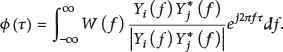
To eliminate the influence of the harmonically related tones in the signals received by different sensors, we estimate the TDOA by maximizing the generalized cross correlation function:

$$\begin{array}{cc}& \varphi \left(\tau \right)={{\displaystyle \int }}_{-\infty }^{\infty }‍W\left(f\right)\frac{Y_i\left(f\right)Y_j^{*}\left(f\right)}{\left|Y_i\left(f\right)Y_j^{*}\left(f\right)\right|}{e}^{j2\pi f\tau }df.\end{array}$$

(8)

As we have mentioned previous, the flight-in-air delay of the radio frequency signal is ignored. Besides, the system delay between the receiving time and the recording time is not considered as well due to the devices variation. Therefore, our approach is approximately synchronization-free. Such two delays, however, are relatively low for the TDOA estimation. The error in TDOA estimation is affected by the signal to noise ratios (SNR). Azaria and Hertz demonstrate the error in [29] and propose the optimal weight function to prefilter the phase noise. Whistle [30] proposes a similar approach to estimate the time delay of the discrete signal emitted at fixed location. It makes the sensor i emit an acoustic signal $S^{\prime }$ to itself and node j and takes the time-of-flight to node i and j into account to achieve synchronization-free TDOA estimation. The speaker, however, may be unavailable in the majority of the current sensor network applications.

If two sensors receive the signal emitted by the same event for a relative long time, for example, multiple sampling periods, the TDOA between them can be estimated. Actually, the TDOA between any one-hop node pair can be estimated twice. One is at the time when the event is approaching the two sensors, while the other one is at the time when the event is leaving them. The case that the event is leaving can be considered as that the event is approaching the sensor field from a reverse direction. Reversing the sampled signals can achieve such an effect.

4. Achieving Localizability with Moving Event

When an event passes through the sensor field, the TDOA observation between any one-hop node pair can be estimated. This section illustrates the basic knowledge of localizability as a preliminary and then proposes the approach to achieve network localizability with moving event. The corresponding localization algorithm is designed in a distributed manner.

4.1. Preliminary

Assume that there are n sensors, including m beacons, which are distributed arbitrarily in a Euclid $R^2$ space. When the sensors are randomly released, any sensor measures the distances to its one-hop neighbors. In a global view, a distance graph $G(V,E)$ that contains all of the nodes in a maximal connected subgraph is achieved, where V denotes the set of the sensor nodes in such a subgraph, and E denotes the set of edges. An edge between nodes i and j in the distance graph G means either the distance between i and j can be measured, or both of them are aware of their own locations (e.g. beacons). Note that the vertex is a specific term of the sensor node in graph G.

A distance graph G is rigid means that it cannot deform its realizations continuously while the distance constraints are preserved. The distance graph G is redundantly rigid if it remains rigid after removing any single edge in G.

Theorem 1 (see [4]).

A graph with $n\ge 4$ vertices is globally rigid in $R^2$ if and only if it is 3-connected and redundantly rigid.

A graph $G=(V,E)$ is called   $k$ -connected (for $k\in N)$ if $|V|>k$ and $G-X$ is connected for every set $X\subseteq V$ with $|X|<k$ . In other words, no two vertices in G are separated by fewer than k other vertices.

Eren et al. [31] further prove that a network is uniquely localizable if and only if its distance graph is globally rigid and it contains at least three beacons.

A node is localizable if its location can be uniquely determined. Yang et al. [7] propose the sufficient condition of the node localizability, as presented in Theorem 2.

Theorem 2 (see [7]).

In a distance graph $G=(V,E)$ , where a set $B\subset V$ of $k\ge 3$ vertices know their locations, a vertex is localizable if it is in a redundantly rigid component inside which there are three vertex-disjoint paths to three distinct vertices in B.

4.2. Localizability with Moving Event

On the foundation of the localizability, we propose the sufficient conditions to achieve node localizability and network localizability with the hybrid distance and TDOA measurement, respectively. The localizable vertices set is defined in Definition 3.

Definition 3 (localizable vertices set).

The localizable vertices set consists of all the initially localizable vertices in a distance graph $G=(V,E)$ , denoted L.

The localizable vertices set differs the localizable part and the nonlocalizable part in a given graph G. Any vertex $l_i\in L$ can receive the acoustic signal emitted by the moving event passing through the area of interest. Therefore, the time-varying location of the event can be determined by the localizable vertices. On this basis, we further explore the localizability of an arbitrary vertex in the nonlocalizable part. Theorem 4 provides the sufficient condition to localize the one-hop neighbor of any localizable vertex.

Theorem 4.

For a localizable vertex $l_i$ and an initially nonlocalizable vertex $v_{\gamma }$ , given the locations of the moving event at time $t_1$ and $t_2$ , as well as the TDOA between $l_i$ and $v_{\gamma }$ , if there is an edge $(v_{\gamma },l_i)$ , where $l_i\in L$ and $l_i$ is not on the trajectory of the event, vertex $v_{\gamma }$ becomes localizable.

Proof.

Consider the event at time $t_1$ and $t_2$ as two virtual vertices, denoted as $\alpha (t_1)$ and $\alpha (t_2)$ . As shown in Figure 4(a), the locations of $\alpha (t_1)$ , $\alpha (t_2)$ and the localizable vertex $l_i$ are known. The distance $d(\alpha (t_1),l_i)$ , $d(\alpha (t_2),l_i)$ , and $d(l_i,v_{\gamma })$ are known, represented by the solid lines. The distance difference between $d(\alpha (t_1),l_i)$ and $d(\alpha (t_2),v_{\gamma })$ can be measured by the TDOA observation as follows:

$$\begin{array}{cc}& d\left(\alpha \left(t_1\right),l_i\right)-d\left(\alpha \left(t_1\right),v_{\gamma }\right)=c{\mathrm{\Delta }}_{l_i,v_{\gamma }}\left(t_1\right),\end{array}$$

(9)

where ${\mathrm{\Delta }}_{l_i,v_{\gamma }}$ denotes the difference of the time between the time that $l_i$ and $v_{\gamma }$ receive the same signal from Event at time $t_1$ . Therefore, $d(\alpha (t_1),v_{\gamma })$ can be determined indirectly, represented by the dotted line in Figure 4(a). Similarly, $d(\alpha (t_2),v_{\gamma })$ can be known. If $\alpha (t_1)$ , $\alpha (t_2)$ , $l_i$ , and $v_{\gamma }$ achieve a redundantly rigid graph, there are three disjoint edges from $v_{\gamma }$ to $\alpha (t_1)$ , $\alpha (t_2)$ , and $l_i$ , respectively. According to Theorem 2, vertex $v_{\gamma }$ becomes localizable.

Figure 4

An example of the graph achieved by the event at $t_1$ , $t_2$ , the localizable vertices set L and nonlocalizable vertices.

If an initially nonlocalizable vertex can receive the signal twice, together with its localizable one-hop neighbor, its location can be uniquely determined by trilateration, as shown in Figure 4(b). However, whether we can derive the TDOA between one-hop neighbors twice is crucial to achieve the node localizability. We will further demonstrate such a problem in Theorem 5.

As the event moves through the sensor field, its coverage is changing as shown in Figure 5. For one-hop vertices i and j, we estimate the TDOA at the occasions that the event is approaching and leaving as illustrated in Section 3. Denote the first time and the last time vertex i receives the signal emitted by the event as $t_i^{(1)}$ and $t_i^{(2)}$ , respectively. Similarly, we have $t_j^{(1)}$ and $t_j^{(1)}$ for vertex j. For $t_1$ and $t_2$ in Theorem 4, we have $t_1=\max \{t_i^{(1)},t_j^{(2)}\}$ and $t_2=\min \{t_i^{(2)},t_j^{(2)}\}$ . When $t_1<t_2$ , there will be a common period that the two nodes can receive the same signal emitted by the event. Therefore, the two TDOA observations can be achieved.

Figure 5

Coverage of the moving event.

Theorem 5.

For any one-hop neighbors, there is a common period that the two vertices can receive the same signal emitted by the event, if the closeted distance form themselves to the trajectory of the event are all smaller than the propagation range of the signal emitted by the event.

Proof.

Obviously, $t_i^{(1)}<t_i^{(2)}$ and $t_j^{(1)}<t_j^{(2)}$ . Denote the propagation range of such a signal as R, while the ranging radius of sensor is r. Due to the high power assumption, $R\gg r$ . Besides, the sound speed c is far larger than the event's moving speed v; that is, $c\gg v$ . Denote that the closet distance from vertex i to the trajectory of the event is $d_i$ . The duration of the receiving signal at sensor i is

$$\begin{array}{cc}& t_i^{\left(2\right)}-t_i^{\left(1\right)}=\frac{2\sqrt{R^2-d_i^2}}{v}.\end{array}$$

(10)

Without loss of generality, we assume that the signal arrives at node i first. The TDOA between one-hop neighbors is bound by r:

$$\begin{array}{cc}& 0<t_j^{\left(1\right)}-t_i^{\left(1\right)}<\frac{r}{c}.\end{array}$$

(11)

To compare the right items in (10) and (11), we have

$$\begin{array}{l}\frac{4c^2\left(R^2-d_i^2\right)}{v^2{r}^2}-1=\frac{4c^2{R}^2-v^2{r}^2-4c^2{d}_i^2}{v^2{r}^2}\\ \approx \frac{4c^2\left(R^2-d_i^2\right)}{v^2{r}^2}.\end{array}$$

(12)

If $R>d_i$ , the left item in (12) is larger than zero. Therefore, $2\sqrt{R^2-d_i^2}/v>r/c$ , and $t_i^{(2)}>t_j^{(1)}$ . As such, we have $t_1<t_2$ .

Therefore, as the event moves through the sensor field, there are at least two occasions that the TDOA between the one-hop neighbors can be estimated. Theorem 6 proposes the sufficient condition for the localizability of any initially nonlocalizable vertex.

Theorem 6.

Given a localizable vertices set L, TDOA between any one-hop neighbors and the time-varying locations of the moving event in the sensor filed, for a nonlocalizable vertex $v_{\gamma }$ , if there is a simple path $P=(v_{\gamma },v_{{\gamma }_1},v_{{\gamma }_2},\dots ,v_{{\gamma }_m},l_i)$ , where $l_i\in L$ and any vertex $v_{{\gamma }_j}$ ( $j\in [1,m]$ ) is not on the trajectory of the event, vertex $v_{\gamma }$ becomes localizable.

Proof.

According to Theorem 4, if $l_i$ is not collinear with $\alpha (t_1)$ and $\alpha (t_2)$ , vertex $v_{{\gamma }_m}$ is localizable. Similarly, for any $v_{{\gamma }_j}$ that is not collinear with $\alpha (t_1)$ and $\alpha (t_2)$ , vertex $v_{{\gamma }_{j-1}}$ is localizable, where $j\in [2,m]$ . In that case, for vertex $v_{{\gamma }_j}$ ( $j\in [1,m-1]$ ). Finally, the vertex $v_{\gamma }$ is localizable if $v_{{\gamma }_1}$ is not collinear with $\alpha (t_1)$ and $\alpha (t_2)$ .

If a localizable vertex $l_i$ is on the trajectory of the event, its successive vertex $v_s$ may be estimated at two symmetrical locations.

Theorem 7.

Given a connected distance graph $G=(V,E)$ and the locations of the moving event at time $t_1$ and $t_2$ , any vertex $v_i\in V$ is localizable if there is at least one beacon in G that is not collinear with the locations of the moving event at $t_1$ and $t_2$ .

Proof.

For any nonlocalizable node, there is at least one simple path to a localizable node, due to the connectivity of G. According to Theorem 6, any nonlocalizable node becomes localizable if its prefix node on the path is not on the trajectory of the event. As for the collinear degradation, there exists the following four cases.

Case 1. If the successive vertex $v_s$ is collinear with the locations of the moving event at $t_1$ and $t_2$ , $v_s$ is localizable (see $v_1$ in Figure 6).

Case 2. If there is a path from the successive vertex $v_s$ to another localizable vertex while each vertex on the path except itself is not collinear with the locations of the moving event at $t_1$ and $t_2$ , $v_s$ is localizable (see $v_2$ in Figure 6).

Case 3. For vertex $v_s$ , if the symmetrical location $v_s^{\prime }$ about the line through $S_1$ , $S_2$ and the $v_{\gamma }$ is in the sensing range of another localizable vertex, it is localizable.

For $v_3$ in Figure 6, if the other possible location $v_3^{\prime }$ is in the sensing range of $l_{i-1}$ , there must exist an edge between them, otherwise, it is located at $v_3$ .

Case 4. If the collinear localizable vertex is not a beacon, vertex $v_s$ is localizable when it doubles its communication range.

For $v_4$ in Figure 6, when the measurement range is doubled, it is easy to demonstrate that there is an edge between itself and a localizable one-hop neighbor of $l_i$ if $l_i$ is not a beacon. Note that such case is quite rare in a randomly deployed WSN. Due to the page limitation, the process of the collinear degradation is omitted in Algorithm 1.

Algorithm 1: Localization with moving event.

Require: neighbor list, time-varying locations of event

  if receive the location of a localized node then

   get the localized nodes with credit less than 3 in neighbor list, denoted as $v_1,v_2,\dots ,N$

   if   $N\le 2$   then

    request the receiving signal of $v_1$

    estimate TDOA between itself and $v_1$

   end if

   trilateration with three references

   compute the credit of its location

   send the localized mark to all of the localized nodes in its neighbor list

   send its location and credit to all of the unlocalized nodes in its neighbor list

  end if

Figure 6

Collinear degradation.

Theorem 8 provides the network localizability condition with two events.

Theorem 8.

Given a connected distance graph $G=(V,E)$ , G is localizable if there is a event passing through the sensor field and at least one vertex whose location is known.

Proof.

Consider about any vertex $i\in V$ at an unknown location. There is at least one path form i to a vertex j whose location is known, due to the connectivity of G. Therefore, G is localizable since any vertex in G is localizable.

Corollary 9.

Given a distance graph $G=(V,E)$ , G is localizable if and only if there is at least one vertex at a known location in any connected component of G.

The proof of Corollary 9 is straightforward from Theorem 8. Thus we omit it in this paper due to the page limitation.

4.3. Design and Implementation

Typically, the implementation of our approach contains four major steps, as shown in Figure 7. Compared to current localization-oriented network adjustment approach, our approach does not require any adjustment if the network is connected in the initial deployment.

Figure 7

Implementation of localization with moving event.

Step 1 (network deployment).

When the sensors are deployed to a given region, each sensor communicates with its one-hop neighbors to obtain the neighbor list and measures its distance to the nodes in such a list. Any beacon sends a message to its one-hop neighbors to mark itself as localizable in its neighbors' neighbor list. Therefore, a distance graph is formed in a global view.

Step 2 (localizability testing).

Node localizability testing is conducted to differ the localizable nodes and nonlocalizable nodes in a network. The localizable nodes are localized in this step.

Step 3 (TDOA estimation).

Any sensor, either the localizable node or the nonlocalizable node, samples the signal with a constant frequency, denoted as   $f_s$ , and records it according to its local time. The nonlocalizable node requests for the receiving signal of its localizable neighbor, if it is necessary to utilize the moving event to localize itself. The TDOA between itself and the localizable neighbor is estimated by generalized cross correlation locally. Note that for the two receiving signals, the TDOA between them can be estimated twice. The one utilizes the original receiving signals to estimate the TDOA when the event is approaching, while the other one utilizes the sampled sequence in reverse order to estimate the TDOA when the event is leaving.

Step 4 (node localization).

The initially nonlocalizable node can be localized via iterative trilateration, when the two TDOAs between itself and its localizable node are achieved. A significant advantage of the trilateration is that it does not require any global information and thus is suitable to be implemented in distributed manner.

The moving events bring redundant edges to achieve the network localizability, and therefore multiple trilateration ordering (given a graph $G=(V;E)$ , if its vertices can be ordered as $v_1,v_2,v_3,\dots ,v_n$ so that $v_1$ , $v_2$ , and $v_3$ induce a complete subgraph and each $v_i,\hspace{0.17em}\hspace{0.17em}i>3$ , is adjacent to at least three vertices $v_j$ where $j<i$ . Such an ordering is the trilateration ordering of G  [3]) can be formed. However, the node localized by inaccurate nodes will be less accurate. The localization error will be accumulated during the process of iterative trilateration. To overcome such a problem, we use the credit as an identification of the localization accuracy. The location of the node with a smaller credit is more accurate. On this basis, the three most accurate nodes in the neighbor list of node i, that is, the three nodes with least credit value, are chosen as the references to implement trilateration.

The credit can be computed by the following rules.

• (1)

The credit of the beacon are set to be 0.

(2)

The credit of the initially localizable node is set to be 1.

(3)

The credits of the time-varying locations of the event are set to be 3.

(4)

The credits of the node localized with three references with credits $c_1$ , $c_2$ , and $c_3$ are set to be $\max \{c_1,c_2,c_3\}+1$ .

Algorithm 1 gives the implementation algorithm at the nonlocalizable node. Any localized node sends its location together with its credit to all of the nonlocalizable nodes in its neighbor list. For a nonlocalizable node, if there is less than 3 localized nodes whose credits are smaller than 3 in its neighbor list, it estimates the TDOA between itself and its one-hop localized neighbor. Therefore, the moving event can be considered as a reference. The node selected 3 references with least credits to localize itself.

5. Performance Evaluation

To validate the correctness and performance of our approach, extensive simulations are conducted in this paper. This section evaluates our approach in terms of TDOA estimation accuracy and localization accuracy, respectively.

5.1. Simulation Setting

We generate a uniformly random network of a thousand nodes in a 1000-by-1000 square region. The sensing radius r of each node is tuned to control the density and connectivity of the network. 100 instances are generated in the simulation, where r ranges from 50 to 100 stage-by-stage with a step length of 0.5 and three beacons are used in each instance. For a node pair, there is an edge between them if the distance between the two members is smaller than the maximal communication radius. The disk model with the Gaussian noise is adopted for distance measurement, where the standard derivation is ${\sigma }_d$ .

To simulate a moving event, we sampled the acoustic signal emitted by a track with a mobile phone equipped near its engine. The track is moving along a straight road with a constant speed of 40 kilometers per hour. The sampling frequency of the mobile phone is 44.1 kHz and the record period is 200 seconds. The average RSS of such a signal is 109.7 dB. The RSS is computed based on the following equation:

$$\begin{array}{cc}& P\left(d\right)=P\left(d_0\right)-10·a·\log d-b,\end{array}$$

(13)

where $a=2$ and $b=11$ for a point source in a seraph space. If the RSS of a node is beyond the threshold $C=50$  dB, such a node can receive the signal. The received signal is simulated by deriving the sampled sequence at the corresponding time with decaying amplitude. We generate a zero-mean Gaussian white noise with a certain Signal Noise Ratio (SNR).

5.2. Accuracy of TDOA Estimation

The TDOA between any one-hop neighbors is estimated. Figure 8 plots the estimation error of all one-hop node pair with a constant SNR of 5 dB. The distance difference between any one-hop neighbors is smaller than the distance between them, due to the triangle inequality. The simulation results show that the maximal estimation error is about 0.08 milliseconds among all the estimations, while its average error is about 0.02 milliseconds. It also indicates that the estimation error is not increased along with the distance difference. The behind reason is that the TDOA is estimated in the frequency domain and hence can alleviate the influence of the energy decay.

Figure 8

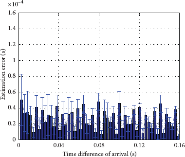
TDOA estimation error with different time delays.

We further change the SNR of the receiving signals from 1 to 10 dB. Note that a lower SNR means a higher noise. The simulation results are shown in Figure 9. It shows that the estimation error gets smaller as the SNR decreases. However, the influence is not significant. The generalized cross correlation approach can effectively eliminate the influence of noise. As shown in the simulation results, our TDOA estimation approach achieves the accuracy of 0.1 milliseconds or better, irrespective of the distance or SNR.

Figure 9

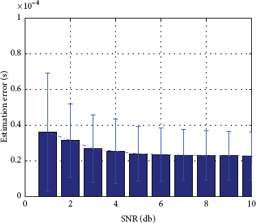
TDOA estimation error with different SNRs.

5.3. Accuracy of Nonlocalizable Nodes Localization

We further study the localization error influenced by the distance measuring error and clock bias. The sensing radius r is fixed at 50 to generate a connected but nonlocalizable network with three beacons. The average node degree of such a network is $\mathrm{4.501}$ , which does not satisfy the globally rigidity condition for a 1000 nodes network obviously. The standard deviations in the distance measurement error is assigned to be ${\sigma }_d=\mathrm{0.01}r,\mathrm{0.02}r,\dots ,\mathrm{0.05}r$ , respectively, where r is the distance measurement range. Figure 10 shows the CDF of localization error with different distance measurement errors. When ${\sigma }_d$ is below $\mathrm{0.01}r$ , about $70\%$ nodes achieve the localization accuracy of $\mathrm{0.02}r$ or better, and about $90\%$ nodes can be localized within $\mathrm{0.04}r$ .

Figure 10

Localization error with different distance measurement noise.

We integrate the results from 100 network instances to evaluate the localization error influence by the network connectivity. Figure 11 plots the relationship between the localization error, the proportion of the initially localizable nodes and the average network connectivity. As the average node degree increases, the proportion of the localizable nodes increases, and the localization error of the nonlocalizable nodes with our approach is significantly reduced from $\mathrm{0.06}r$ to $\mathrm{0.02}r$ . Besides, the localization takes about 3 minutes for each process among 100 instances on average with a consumer PC.

Figure 11

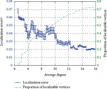
Localization error with different network density.

6. Conclusion

Localization is an essential service in WSN applications. This paper is the first work that focuses on the localizability problem with the hybrid TDOA and distance measurement. We propose the sufficient condition to achieve the localizability in an initially nonlocalizable WSN via a moving passive event, as well as the corresponding algorithm in a distributed manner. Besides, we propose an approximately synchronization-free TDOA localization to improve the accuracy of our approach. The localization accuracy achieves $\mathrm{0.02}r$ under the common distance measurement. Following this paper, we intend to extend our current work to real implementation in a large scale WSN.