The Effect of First-Order Bending Resonance of Wheelset at High Speed on Wheel-Rail Contact Behavior

Abstract

The first-order bending deformation of wheelset is considered in the modeling vehicle/track coupling dynamic system to investigate its effect on wheel/rail contact behavior. In considering the effect of the first-order bending resonance on the rolling contact of wheel/rail, a new wheel/rail contact model is derived in detail in the modeling vehicle/track coupling dynamic system, in which the many intermediate coordinate systems and complex coordinate system transformations are used. The bending mode shape and its corresponding frequency of the wheelset are obtained through the modal analysis by using commercial software ANSYS. The modal superposition method is used to solve the differential equations of wheelset motion considering its flexible deformation due to the first-order bending resonance. In order to verify the present model and clarify the influence of the first-order bending deformation of wheelset on wheel/track contact behavior, a harmonic track irregularity with a fixed wavelength and a white-noise roughness are, respectively used as the excitations in the two models of vehicle-rail coupling dynamic system, one considers the effect of wheelset bending deformation, and the other does not. The numerical results indicate that the wheelset first-order bending deformation has an influence on wheel/rail rolling contact behavior and is easily excited under wheel/rail roughness excitation.

1. Introduction

The development of high-speed railway is associated with dynamic problems, for example, the wear of their wheels/rails. When a train with polygonal wheels due to wear operates on a track at high speed, the train and the track vibrate fiercely in an extensive frequency range. The wheel polygonal wear excites the strong dynamic behavior of the vehicle/track structures in mid- and high-frequency ranges. In the extensive experiments conducted on China metro lines by Jin et al. [1], the test results showed that all of the wheels of one type of metro trains in service present the 9th-order polygonal wear, and the excitation frequency of polygonal wheel was close to the first-order bending resonance frequency of the wheelset. The root of the 9th order polygonal wear was attributed to the first-order bending resonance occurring of wheelset in operation, as indicated in Figure 1. Now, the problem of wheel polygonal wear is very common on the existing high-speed trains in China. The mechanism of this phenomenon has not been explained perfectly until now, and it also has become one of the most difficult problems of the wheel-rail system to be solved. The wheel polygon due to wear usually takes a long time and so far cannot be reproduced through the numerical simulation due to the existing insufficiently advanced theoretical models for railway vehicle coupling with track.

Figure 1:

The root cause of harmonic wear of metro wheels [1].

The dynamics analysis of railway vehicle by using the existing rigid multibody dynamics models for vehicle/track coupling system is limited in the low-frequency domain of 0–20 Hz [2]. An effective way to broaden the analysis frequency range is to take the structural flexibility of vehicle/track into consideration in modeling the vehicle/track system [3–6]. And the key part in modeling structural flexibility of the vehicle/track is to consider the effect of the flexibility of wheelset on the rolling contact of wheelset/rail.

Many scholars have carried out a lot of researches on the vehicle/track dynamic system modeling that considers the effect of flexible wheelset. In [5], the wheelset was treated as a lumped and discrete structure by Popp et al. In [4, 6–8], the existing models of the flexible wheelset were continuous models. A vehicle/track dynamic model developed by Meinders considering wheelset flexibility was based on the cosimulation of finite element analysis software ANSYS and multibody dynamics simulation software NEWEUL [9, 10]. Baeza et al. [11–13] proposed a numerical dynamic system model originating from a rotating elastic cylinder model, taking inertial effect and effect of Coriolis force into account.

In terms of wheel/rail rolling contact modeling, the effect of wheelset deformation in mid- and high-frequency ranges should not be neglected [14]. Though many literatures presented different methods to model flexible wheelsets, the detailed derivations of rolling contact geometry of a flexible wheelset and a pair of flexible rails and the detailed calculations and discussions on the effect of the high-frequency bending of wheelset on the rolling contact behavior were not given. This is a very difficult research. The influence exerted by the wheelset bending formation is much concerned with wheelset polygonal wear. In [15], the effect of wheelset flexible deformation on the creepages and the creep forces in static state was indicated to be significant. The flexible deformation of a wheelset in service always contains mid- and high-frequency components. The rolling contact behavior of the wheel/rail caused by wheelset deformation would be in mid- and high-frequency ranges, which brings a great difficulty into the on-line calculation of wheel/rail contact geometry. And the existing models for the wheel/rail contact geometry are not suitable for the model with flexible wheelsets and need to be further improved.

In this paper, a new wheel/rail contact model is developed to consider the effect of the wheelset first-order bending deformation on the wheel/rail rolling contact behavior. The main object is to analyze the effect of wheelset flexibility on the wheel/rail contact behavior mainly in mid-frequency range. The mid-frequency components of the excitation from the wheel/rail interaction system are filtered by the suspension system, and the wheel/rail mid-frequency excitation cannot easily excite the flexibility of the car-body and bogies. Hence, the influence of the structural flexibility of car-body and bogies is ignorable in this present paper. In Section 2, the model of the flexible wheelset and the wheel/rail contact model are introduced. In Section 3, a harmonic track irregularity with a fixed wavelength and white-noise roughness of the rail are adopted as the excitations to analyze the effect of the wheelset flexibility.

2. Modeling

2.1. Vehicle/Track Model

Conventional vehicle system models consist of one carriage, two bogies, and four wheelsets, which are considered as rigid bodies or lumped masses connected by spring-damping systems. A ballasted track is usually modeled as a triple-layer model of discrete elastic support. The rail is modeled as a Timoshenko beam on elastic point supporting foundation. The two ends of the calculation rail are simply supported. The vertical and lateral bending deformations and twisting of the rails are taken into account. The sleepers are modeled as rigid bodies, and the ballasts are regarded as discrete equivalent bodies. The equivalent spring-damping systems are used as the connections between the rails and the sleepers, the sleepers and the equivalent ballast bodies, and the ballast bodies and the subgrade. Figure 2 illustrates such a model of the vehicle and the track. Its detailed description and the derivation of motion equations refer to the published papers, for example, [16–18]. The important parameters of the vehicle and the track used in this paper calculation are given in Table 1.

Table 1:

 

Physical parameter	Value	Unit	Notation
M c	33.766 × 103	kg	Car-body mass
M bi	2.4 × 103	kg	The ith bogie mass
M wi	1.85 × 103	kg	The ith wheelset mass
C ty	20 × 103	Ns/m	The equivalent lateral damping of secondary suspension (considering damping of lateral shock absorber joint)
K ty	18.13 × 106	N/m	The equivalent lateral stiffness of secondary suspension (considering stiffness of lateral shock absorber joint and lateral stiffness of air spring)
C tz	40 × 103	Ns/m	The equivalent vertical damping of secondary suspension (considering vertical damping of air spring)
K tz	299 × 103	N/m	The equivalent vertical stiffness of secondary suspension (considering vertical stiffness of air spring)
C fy	0	Ns/m	The equivalent lateral damping of primary suspension
K fy	6.47 × 106	N/m	The equivalent lateral stiffness of primary suspension (considering the lateral stiffness locating node of the axle-box rotary arm)
C fz	15 × 103	Ns/m	The equivalent vertical damping of primary suspension (considering damping of vertical shock absorber joint)
K fz	6.076 × 106	N/m	The equivalent vertical stiffness of primary suspension (considering stiffness of vertical shock absorber joint and steel spring)
M r	60.64	kg/m	Rail mass per unit length
M s	349	kg	Mass of sleeper
M b	466	kg	Mass of ballast element
L s	0.6	m	Sleeper bay
E	2.06 × 1011	N/m2	Young's modulus
K pLi	20 × 106	N/m	Lateral stiffness of the ith pad
C pLi	5 × 104	N/m	Lateral damping of the ith pad
K pVi	40 × 106	N/m	Vertical stiffness of the ith pad
C pVi	5 × 104	N/m	Vertical damping of the ith pad
K bv(L, R)i	80 × 106	N/m	Vertical stiffness between sleeper and the ith ballast element
C bv(L, R)i	1 × 105	Ns/m	Vertical damping between sleeper and the ith ballast element
K w	78 × 106	N/m	Vertical stiffness between sleeper and the ith ballast element
C w	8 × 104	Ns/m	Vertical damping between sleeper and the ith ballast element
K fv(L, R)i	65 × 106	N/m	Vertical stiffness between road bed and the ith ballast element
C fv(L, R)i	31000	N/m	Vertical damping between road bed and the ith ballast element

Figure 2:

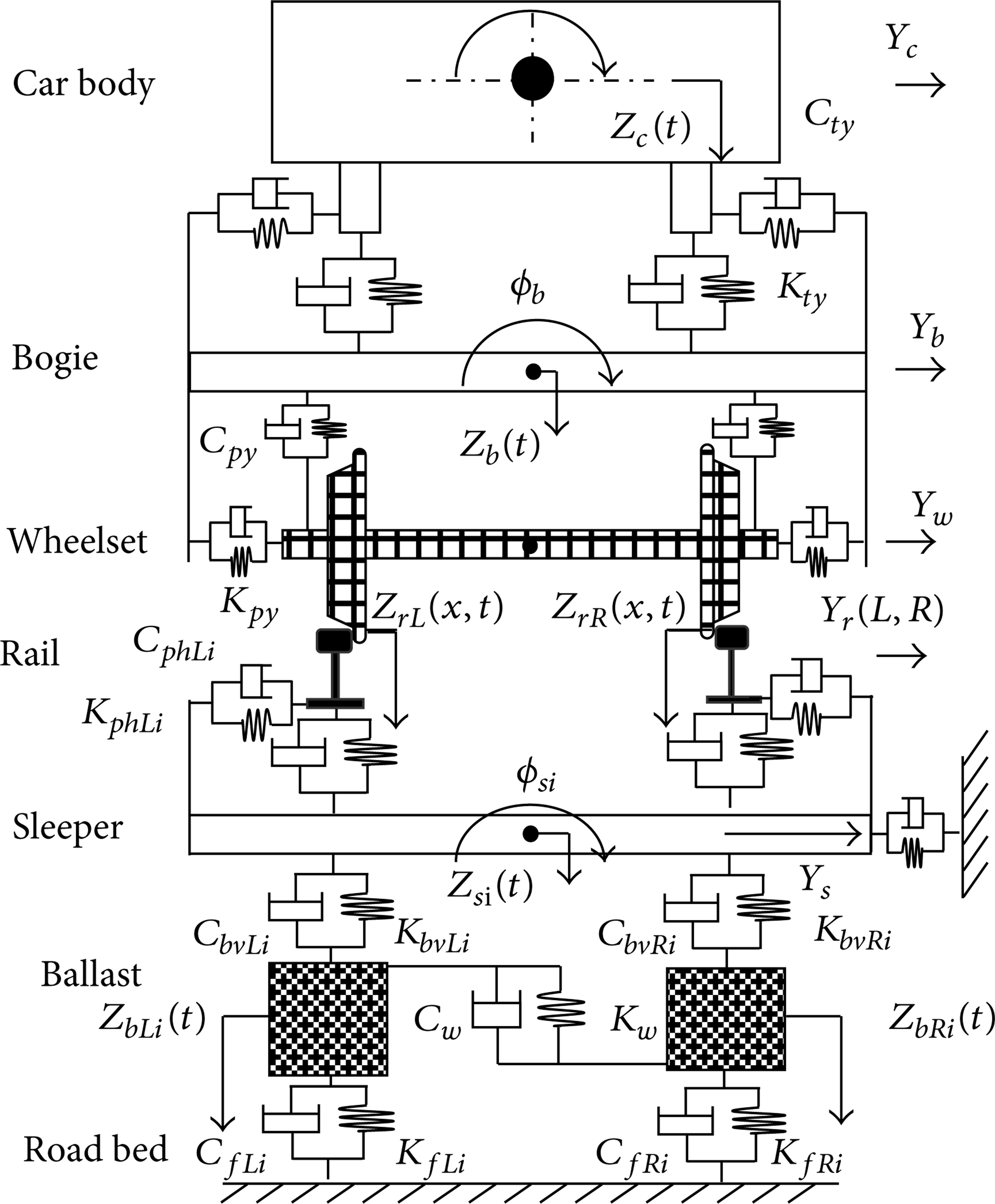
Vehicle/track coupling model (elevation).

2.2. Flexible Wheelset Model

The flexible wheelset modeling mainly considers the contribution of the first-order bending deformations of the wheelset axle in the two planes, perpendicular and parallel to the track level plane, respectively, and neglects their crossing effect. The wheelset modes are calculated by using the finite element software ANSYS. The corresponding resonance frequency of the first-bending, shown in Figure 3, is about 117 Hz. This mode function will be used in the analytical solution to the partial differential equations of the wheelset deformation based on the modal superposition method [16].

Figure 3:

Force analysis diagram of the flaxible wheelset.

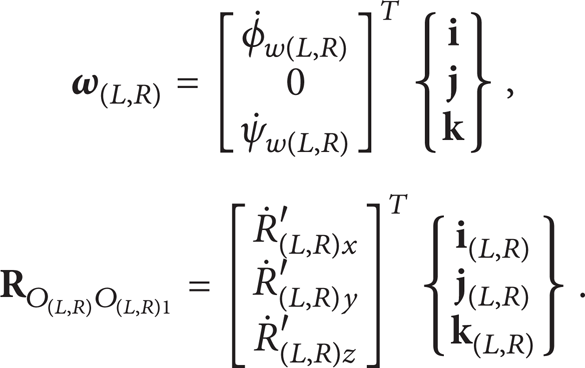
Figure 3 indicates the force system on the flexible wheelset. O _fL and O _fR are, respectively, the left and right points of the application of the primary suspension forces on the axle. O _CL and O _CR are, respectively, the left and right contact points of wheel/rail. O indicates the origin of the coordinate system O-XYZ that is a coordinate system with a translational motion along with a tangent track central line at the vehicle speed. If the vehicle speed is a constant, this coordinate system is an inertial coordinate system, therefore, regarded as an absolute coordinate system (geodetic coordinate system).

Based on the above assumptions that the wheels are regarded as the rigid bodies and perpendicular to the axle central lines at their centers, their spatial poses are determined by the positions of nominal rolling circle centers and the directions of the normal lines through nominal rolling circle centers on the deformed axle centerline. The wheelset axle is modeled as an Euler-Bernoulli beam. So according to the force analysis diagram of the wheelset given in Figure 3, the left and right wheel/rail forces are, respectively, translated to the nominal circle centers, O _L and O _R . Such a force translation introduces the additional moments applied to the axle. The additional moments are the products of the wheel/rail forces and the distance vector between the wheel/rail contact points and the rolling circle centers. Then, the force analysis diagrams in the two planes of the wheelset axle could be obtained, as shown in Figures 4(a) and 4(b), based on which the differential equations of the axle can be established.

Figure 4:

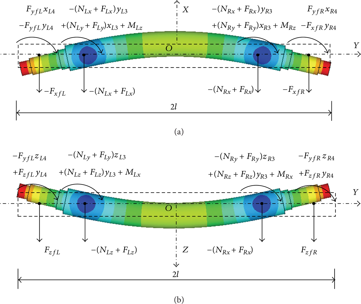
Force analysis diagrams (a) in the X-Y plane parallel to the track level plane and (b) in the Z-Y plane parallel to the track level plane.

The partial differential equations of the wheelset in bending deformation in the two planes, (1) and (2), give the equations for the perpendicular and the parallel planes to the track level plane, respectively, as follows

$E{I}_z\frac{{\partial }^{\mathrm{4}}x(y,t)}{\partial y^{\mathrm{4}}}+\rho A\frac{{\partial }^{\mathrm{2}}x(y,t)}{\partial t^{\mathrm{2}}}=-Q_x\left(y,t\right)-\frac{\partial M_z\left(y,t\right)}{\partial y},$

(1)

$E{I}_x\frac{{\partial }^{\mathrm{4}}z(y,t)}{\partial y^{\mathrm{4}}}+\rho A\frac{{\partial }^{\mathrm{2}}z(y,t)}{\partial t^{\mathrm{2}}}=Q_z\left(y,t\right)-\frac{\partial M_x\left(y,t\right)}{\partial y}.$

(2)

In (1) and (2), Q _x (y, t) and Q _z (y, t) are, respectively, given as

$\begin{array}{c}-Q_x\left(y,t\right)=\left(N_{Lx}+F_{Lx}\right)\delta \left(y-y_{L\mathrm{3}}\right)+F_{xfL}\delta \left(y-y_{L4}\right)+\left(N_{Rx}+F_{Rx}\right)\delta \left(y-y_{R\mathrm{3}}\right)+F_{xfR}\delta \left(y-y_{R\mathrm{4}}\right),\\ Q_z\left(y,t\right)=-\left(N_{Lz}+F_{Lz}\right)\delta \left(y-y_{L\mathrm{3}}\right)+F_{zfL}\delta \left(y-y_{L\mathrm{4}}\right)-\left(N_{Rz}+F_{Rz}\right)\delta \left(y-y_{R\mathrm{3}}\right)+F_{zfR}\delta \left(y-y_{R\mathrm{4}}\right)+G\delta \left(y-\mathrm{0}\right).\end{array}$

(3)

M _z (y, t) and M _x (y, t) are, respectively, given as

$M_z\left(y,t\right)=\left(-\left(N_{Lx}+F_{Lx}\right)y_{L\mathrm{3}}+\left(N_{Ly}+F_{Ly}\right)x_{L\mathrm{3}}+M_{Lz}\right)\times \delta \left(y-y_{L\mathrm{3}}\right)+\left(-\left(N_{Rx}+F_{Rx}\right)y_{R\mathrm{3}}+\left(N_{Ry}+F_{Ry}\right)x_{R\mathrm{3}}+M_{Rz}\right)\times \delta \left(y-y_{R\mathrm{3}}\right)+\left(-F_{xfL}{y}_{L\mathrm{4}}+F_{yfL}{x}_{L\mathrm{4}}\right)\delta \left(y-y_{L\mathrm{4}}\right)+\left(-F_{xfR}{y}_{R\mathrm{4}}+F_{yfR}{x}_{R\mathrm{4}}\right)\delta \left(y-y_{R\mathrm{4}}\right),$

(4)

$M_x\left(y,t\right)=\left(-\left(N_{Ly}+F_{Ly}\right)z_{L3}+\left(N_{Lz}+F_{Lz}\right)y_{L3}+M_{Lx}\right)\times \delta \left(y-y_{L3}\right)+\left(-\left(N_{Ry}+F_{Ry}\right)z_{R3}+\left(N_{Rz}+F_{Rz}\right)y_{R3}+M_{Rx}\right)\times \delta \left(y-y_{R3}\right)+\left(-F_{yfL}{z}_{L4}+F_{zfL}{y}_{L4}\right)\delta \left(y-y_{L4}\right)+\left(-F_{yfR}{z}_{R4}+F_{zfR}{y}_{R4}\right)\delta \left(y-y_{R4}\right).$

(5)

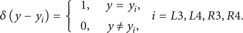
The function δ(⋅) in (3)∼(5) reads as

$\delta \left(y-y_i\right)=\{\begin{array}{ccc}\begin{array}{c}\mathrm{1},\\ \mathrm{0},\end{array}& \begin{array}{c}y=y_i,\\ y\ne y_i,\end{array}& i=L\mathrm{3},L\mathrm{4},R\mathrm{3},R\mathrm{4}.\end{array}$

(6)

The boundary conditions of (1) and (2) are given as

$\begin{array}{c}{x}^{\mathrm{\prime \prime }}\left(-l_{\text{axle}},t\right)=x^{\mathrm{\prime \prime \prime }}\left(-l_{\text{axle}},t\right)=\mathrm{0},\\ x^{\mathrm{\prime \prime }}\left(l_{\text{axle}},t\right)=x^{\mathrm{\prime \prime \prime }}(l_{\text{axle}},t)=\mathrm{0},\\ z^{\mathrm{\prime \prime }}\left(-l_{\text{axle}},t\right)=z^{\mathrm{\prime \prime \prime }}\left(-l_{\text{axle}},t\right)=\mathrm{0},\\ z^{\mathrm{\prime \prime }}\left(l_{\text{axle}},t\right)=z^{\mathrm{\prime \prime \prime }}\left(l_{\text{axle}},t\right)=\mathrm{0},\end{array}$

(7)

where “^′” means one-order partial derivative with respect to y coordinate.

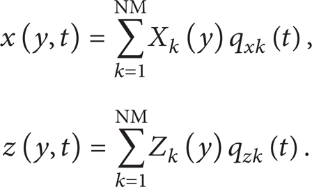
Based on the modal superposition principle, the solutions to (1) and (2) are, respectively, given as

$\begin{array}{c}x(y,t)=\sum _{k=\mathrm{1}}^{\text{NM}}{X}_k\left(y\right)q_{xk}\left(t\right),\\ z(y,t)=\sum _{k=\mathrm{1}}^{\text{NM}}{Z}_k\left(y\right)q_{zk}\left(t\right).\end{array}$

(8)

Using the normalized modal functions which are mutually orthogonal, we have that

${\stackrel{‥}{q}}_{xk}+{\lambda }_{xk}^{\mathrm{2}}{q}_{xk}=P_{xk},\hspace{1em}\hspace{1em}{\stackrel{‥}{q}}_{zk}+{\lambda }_{zk}^{\mathrm{2}}{q}_{zk}=P_{zk}.$

(9)

P _xk and P _zk are, respectively, given as

$\begin{array}{c}{P}_{xk}=\left(N_{Lx}+F_{Lx}\right)X_k\left(y_{L\mathrm{3}}\right)+F_{xfL}{X}_k\left(y_{L\mathrm{4}}\right)+\left(N_{Rx}+F_{Rx}\right)X_k\left(y_{R\mathrm{3}}\right)+F_{xfR}{X}_k\left(y_{R\mathrm{4}}\right)+\left(-\left(N_{Lx}+F_{Lx}\right)y_{L\mathrm{3}}+\left(N_{Ly}+F_{Ly}\right)x_{L\mathrm{3}}+M_{Lz}\right)\times X_k^{\prime }\left(y_{L\mathrm{3}}\right)+\left(-\left(N_{Rx}+F_{Rx}\right)y_{R\mathrm{3}}+\left(N_{Ry}+F_{Ry}\right)x_{R\mathrm{3}}+M_{Rz}\right)\times X_k^{\prime }\left(y_{R\mathrm{3}}\right)+\left(-F_{xfL}{y}_{L\mathrm{4}}+F_{yfL}{x}_{L\mathrm{4}}\right)X_k^{\prime }\left(y_{L\mathrm{4}}\right)+\left(-F_{xfR}{y}_{R\mathrm{4}}+F_{yfR}{x}_{R\mathrm{4}}\right)X_k^{\prime }\left(y_{R\mathrm{4}}\right),\\ P_{zk}=-\left(N_{Lz}+F_{Lz}\right)Z_k\left(y_{L\mathrm{3}}\right)+F_{zfL}{Z}_k\left(y_{L\mathrm{4}}\right)-\left(N_{Rz}+F_{Rz}\right)Z_k\left(y_{R\mathrm{3}}\right)+F_{zfR}{Z}_k\left(y_{R\mathrm{4}}\right)+G{Z}_k\left(\mathrm{0}\right)\times \left(-\left(N_{Ly}+F_{Ly}\right)z_{L\mathrm{3}}+\left(N_{Lz}+F_{Lz}\right)y_{L\mathrm{3}}+M_{Lx}\right)\times Z_k^{\prime }\left(y_{L\mathrm{3}}\right)+\left(-\left(N_{Ry}+F_{Ry}\right)z_{R3}+\left(N_{Rz}+F_{Rz}\right)y_{R\mathrm{3}}+M_{Rx}\right)\times Z_k^{\prime }\left(y_{R\mathrm{3}}\right)+\left(-F_{yfL}{z}_{L\mathrm{4}}+F_{zfL}{y}_{L\mathrm{4}}\right)Z_k^{\prime }\left(y_{L\mathrm{4}}\right)+\left(-F_{yfR}{z}_{R\mathrm{4}}+F_{zfR}{y}_{R\mathrm{4}}\right)Z_k^{\prime }\left(y_{R\mathrm{4}}\right).\end{array}$

(10)

In addition, the contribution of the rigid modes to the wheelset motion is also taken into account. The total displacements of the wheelset in the two planes, which are, respectively, parallel and perpendicular to the track level plane, read as

$\begin{array}{c}x\left(y,t\right)=\sum _{k=\mathrm{1}}^{\text{NME}}{X}_{Ek}\left(y\right)q_{Exk}\left(t\right)+\sum _{k=\mathrm{1}}^{\text{NMR}}{X}_{Rk}\left(y\right)q_{Rxk}\left(t\right),\\ z(y,t)=\sum _{k=\mathrm{1}}^{\text{NME}}{Z}_{Ek}\left(y\right)q_{Ezk}\left(t\right)+\sum _{k=\mathrm{1}}^{\text{NMR}}{Z}_{Rk}\left(y\right)q_{Rzk}\left(t\right).\end{array}$

(11)

The elastic mode number is given as NME = NM = 1, and the rigid model number is given as NMR = 2. The rigid modal functions read as

$\begin{array}{c}{X}_{Rk}\left(y\right)=-Z_{Rk}\left(y\right)=\{\begin{array}{cc}-\sqrt{\frac{\mathrm{1}}{\rho A}},\hfill & k=\mathrm{1},\hfill \\ -\sqrt{\frac{\mathrm{3}}{\rho A}}\left(\mathrm{1}-\frac{y}{l_{\text{axle}}}\right),\hfill & k=\mathrm{2}.\hfill \end{array}\end{array}$

(12)

The wheelset bending deformation in the two planes has an influence on the primary suspension forces in the directions of X- and Z-axes, which read, respectively, as

$\begin{array}{c}{F}_{xf\left(L,R\right)i}\hspace{0.17em}=K_{fx}\left(\pm l_b{\psi }_b\left(t\right)+H_{bw}{\beta }_b\left(t\right)-x_i\left(\mp l_w,t\right)\right)\hspace{1em}\phantom{\text{k}}+C_{fx}\left(\pm l_b{\dot{\psi }}_b\left(t\right)+H_{bw}{\dot{\beta }}_b\left(t\right)-{\dot{x}}_i\left(\mp l_w,t\right)\right),\\ F_{zf\left(L,R\right)i}\hspace{0.17em}=K_{fz}\left(Z_b\left(t\right)-z_i\left(\mp l_w,t\right)+{\left(-\mathrm{1}\right)}^i{l}_b{\beta }_b\left(t\right)\mp l_b{\varphi }_b\left(t\right)\right)\hspace{1em}\phantom{\text{k}}+C_{fz}\left({\dot{Z}}_b\left(t\right)-{\dot{z}}_i\left(\mp l_w,t\right)+{\left(-\mathrm{1}\right)}^i{l}_b{\dot{\beta }}_b\left(t\right)\mp l_b{\dot{\varphi }}_b\left(t\right)\right).\end{array}$

(13)

The lateral primary suspension forces on the four wheelsets read as

$F_{yf\left(L,R\right)i}\hspace{0.17em}=K_{fy}\left(u_{yi}\left(\mp l_w,t\right)-Y_b\left(t\right)+H_{bw}{\varphi }_b\left(t\right)+{\left(-\mathrm{1}\right)}^i{l}_b{\psi }_b\left(t\right)\right)\hspace{0.17em}+C_{fy}\left({\dot{u}}_{yi}\left(\mp l_w,t\right)-{\dot{Y}}_b\left(t\right)+H_{bw}{\dot{\varphi }}_b\left(t\right)+{\left(-\mathrm{1}\right)}^i{l}_b{\dot{\psi }}_b\left(t\right)\right).$

(14)

The effect of the wheelset bending deformation on the lateral primary suspension forces is neglected. They are mainly influenced by the wheelset rigid motion in the Y-direction. Substituting (11) into (13), the components of the primary suspension forces in the directions of X- and Z-axes are written as follows:

$\begin{array}{c}{F}_{xf\left(L,R\right)i}\hspace{0.17em}=K_{fx}(-(\phantom{\sum _{k=\mathrm{1}}^{\text{NMR}}{X}_{Rk}\left(\mp l_w\right)q_{Rxki}\left(t\right)}\sum _{k=\mathrm{1}}^{\mathrm{2}}{X}_{Ek}\left(\mp l_w\right)q_{Exki}\left(t\right)\hspace{1em}+\sum _{k=\mathrm{1}}^{\text{NMR}}{X}_{Rk}\left(\mp l_w\right)q_{Rxki}\left(t\right))\pm l_b{\psi }_b\left(t\right)+H_{bw}{\beta }_b\left(t\right)\phantom{\sum _{k=\mathrm{1}}^{\mathrm{2}}{X}_{Ek}\left(\mp l_w\right)q_{Exki}\left(t\right)})\hspace{0.17em}+C_{fx}(-(\phantom{\sum _{k=\mathrm{1}}^{\text{NMR}}{X}_{Rk}\left(\mp l_w\right){\dot{q}}_{Rxki}\left(t\right)}\sum _{k=\mathrm{1}}^{\mathrm{2}}{X}_{Ek}\left(\mp l_w\right){\dot{q}}_{Exki}\left(t\right)\hspace{1em}\phantom{\pm l_b{\dot{\psi }}_b\left(t\right)+++}+\sum _{k=\mathrm{1}}^{\text{NMR}}{X}_{Rk}\left(\mp l_w\right){\dot{q}}_{Rxki}\left(t\right))\hspace{1em}\phantom{\pm l_b{\dot{\psi }}_b\left(t\right)++}\pm l_b{\dot{\psi }}_b\left(t\right)+H_{bw}{\dot{\beta }}_b\left(t\right)\phantom{\sum _{k=\mathrm{1}}^{\mathrm{2}}{X}_{Ek}\left(\mp l_w\right){\dot{q}}_{Exki}\left(t\right)}),\\ F_{zf\left(L,R\right)i}=K_{fz}(Z_b\left(t\right)-(\sum _{k=\mathrm{1}}^{\mathrm{2}}{Z}_{Ek}\left(\mp l_w\right)q_{Ezki}\left(t\right)\phantom{=K_{fz}+\phantom{Z_b\left(t\right)-+}\phantom{+}}+\sum _{k=\mathrm{1}}^{\text{NMR}}{Z}_{Rk}\left(\mp l_w\right)q_{Rzki}\left(t\right))\phantom{+}+{\left(-\mathrm{1}\right)}^i{l}_b{\beta }_b\left(t\right)\mp l_b{\varphi }_b\left(t\right)\phantom{\sum _{k=\mathrm{1}}^{\mathrm{2}}{Z}_{Ek}\left(\mp l_w\right)q_{Ezki}\left(t\right)})+C_{fz}({\dot{Z}}_b\left(t\right)-(\sum _{k=\mathrm{1}}^{\mathrm{2}}{Z}_{Ek}\left(\mp l_w\right){\dot{q}}_{Ezki}\left(t\right)+\sum _{k=\mathrm{1}}^{\text{NMR}}{Z}_{Rk}\left(\mp l_w\right){\dot{q}}_{Rzki}\left(t\right))+{\left(-\mathrm{1}\right)}^i{l}_b{\dot{\beta }}_b\left(t\right)\mp l_b{\dot{\varphi }}_b\left(t\right)\phantom{\sum _{k=\mathrm{1}}^{\mathrm{2}}{Z}_{Ek}\left(\mp l_w\right){\dot{q}}_{Ezki}\left(t\right)}).\end{array}$

(15)

The flexible wheelset model is successfully coupled with the bogie through (14) and (15). The calculation formulas of the wheel/rail contact forces are to be discussed below.

2.3. Wheel/Rail Rolling Contact Model

2.3.1. Description of Coordinate Systems for Wheel/Rail Rolling Contact Calculation

It is complex and tedious to carry out the rolling contact behavior calculation of a flexible wheelset running on a pair of rails in service. The calculation is carried out with the aid of the transformations of multicoordinate systems. A wheel/rail rolling contact model considering flexible wheelset effect is much different from that without considering flexible wheelset effect.

Figure 5 indicates a detailed contact geometry description of a flexible wheelset in rolling contact with a pair of rails, the global coordinate system, and the local coordinate systems used in the rolling contact calculation. In Figure 4, the rolling angles, ϕ_{w(L, R)}, are, actually, the projections of the rotation angles of the normal line of the axle cross-section at the wheel nominal rolling circle centers in the O-ZY plane, but the yawing angles ψ_{w(L, R)} of the wheels, which are the projections in the O-XY plane, are not shown in the figure and can be described in the top view of Figure 5 that is omitted here.

Figure 5:

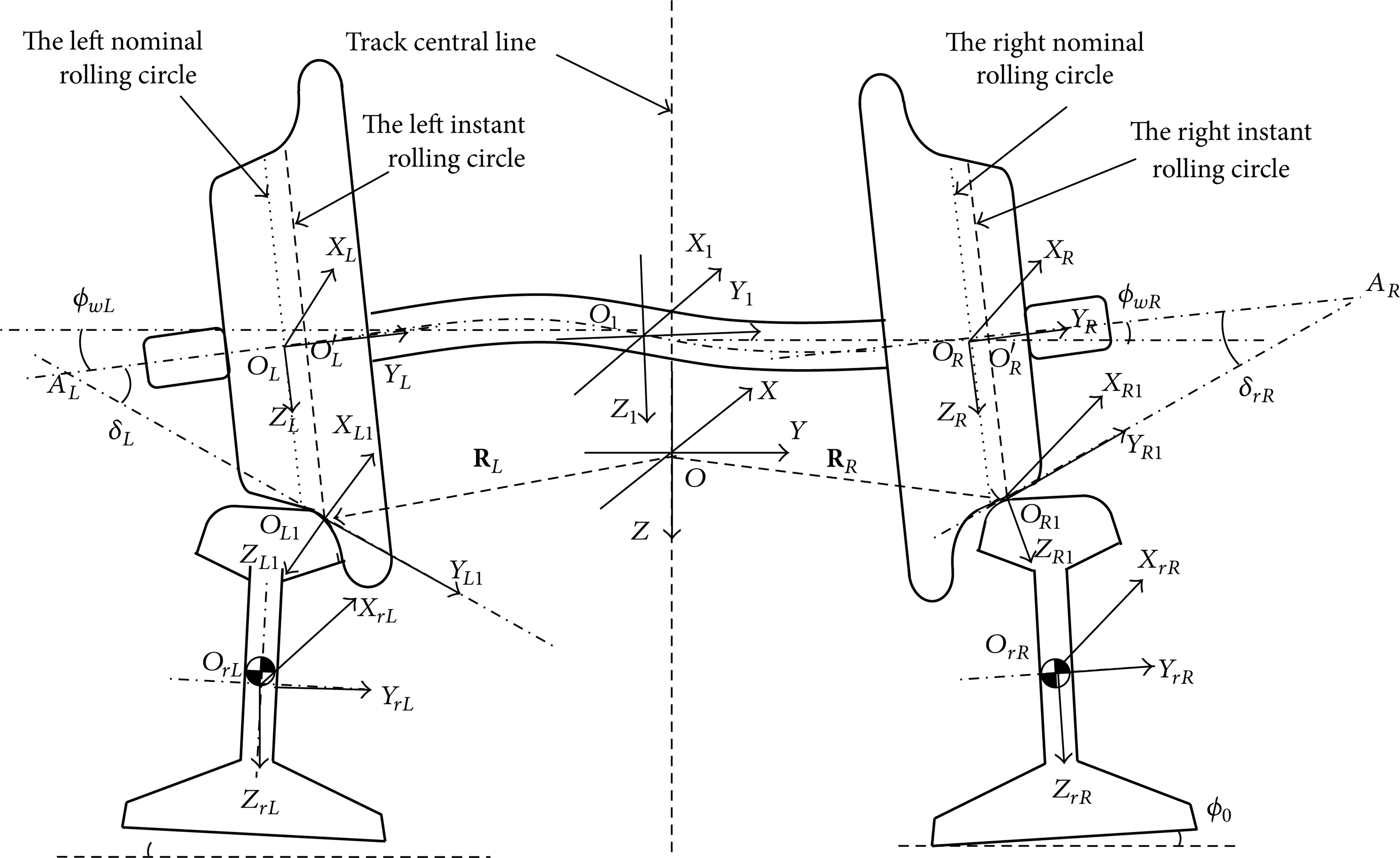
A flexible wheelset in rolling contact with a pair of rail.

The left and right contact points are regarded as, respectively, the origins O_L1 and O_R1 of the local coordinates O_{(L, R) 1}-X_{(L, R) 1}Y_{(L, R) 1}Z_{(L, R) 1}. o _L ′ and o _R ′ are the centers of the left and right instant rolling circles, respectively. The two auxiliary lines are created, and they are, respectively, perpendicular to the left and right instant circles and pass through the centers o _L ′ and o _R ′. These two auxiliary lines, respectively, intersect with the common planes of the wheel/rail contact surfaces, and points A _L and A _R are, respectively, their intersection points, as indicated in Figure 5. Making a line connects point A _L to the left contact point O_L1 and the other line connects point A _R to the left contact point O_R1. The included angle between line A _L O_L1 and line A _L o _L ′ and the one between line A _R O_R1, and line A _R o _R ′ are exactly the contact angles δ _L and δ _R , respectively. Each coordinate system in Figures 2 and 4 has the following detailed description and requirements.

1. O – XYZ: this coordinate system is illustrated in Section 2.2. Its base vector is that e = [i, j, k]. Its unit vectors, i, j, and k are, respectively, in the longitudinal, vertical and lateral directions of the tangent track.

2. O₁-X₁Y₁Z₁: it is a translating coordinate system that is always parallel to the coordinate system O-XYZ, as indicated in Figure 5. It translates with the wheelset mass center. Its base vector is that e₁ = [i₁, j₁, k₁].

3. O_{(L, R)}-X_{(L, R)}Y_{(L, R)}Z_{(L, R)}: they are the local coordinate systems attached to the two rigid wheels, as indicated in Figure 5. Their origins O _L and O _R are at the centers of the nominal rolling circles of the left and right wheels, respectively, which means that their poses are determined by the wheel poses and their Y_{(L, R)} axes are always perpendicular to the corresponding nominal rolling circle planes. The nominal rolling circles of the left and right wheels coincide with the planes O _L -X _L Z _L and O _R -X _R Z _R , respectively. But the rolling motions of the left and right wheels are around the axes X _L and X _R , respectively, and their yawing motions are around the axes Z _L and Z _R , respectively. So the axes X _L and X _R are always parallel to the horizontal plane, and the axes Z _L and Z _R are always parallel to the vertical plane. Their base vectors are that e_{(L, R)} = [i_{(L, R)}, j_{(L, R)}, k_{(L, R)}]. The unit vectors i_(·), j_(·), and k_(⋅) indicate the directions of the axes X_(·), Y_(·), and Z_(·), respectively.

4. O_{(L, R) 1}-X_{(L, R) 1}Y_{(L, R) 1}Z_{(L, R) 1}: their axes Y_L1 and Y_R1, respectively, coincide with the lines A _L O_L1 and A _R O_R1, as indicated in Figure 5. The planes O_L1-X_L1Y_L1 and O_R1-X_R1Y_R1 coincide with the common tangent planes of the contact surfaces of the left and right wheels/rails, respectively. The axes Z_L1 and Z_R1 coincide with the common normal lines of the contact surfaces of the left and right wheels/rails, respectively. Their base vectors are that e_{(L, R) 1} = [i_{(L, R) 1}, j_{(L, R) 1}, k_{(L, R) 1}].

5. O_{r(L, R)}-X_{r(L, R)}Y_{r(L, R)}Z_{r(L, R)}: these two coordinate systems are used to describe the configurations and motions of the left and right rail cross-sections which are assumed to be rigid. Their origins are fixed at the left and right rail cross-session centers, O _rL and O _rR , and their rotation and translation are determined by those of the rail cross-sections. Their base vectors are, that, e_{r(L, R)} = [i_{r(L, R)}, j_{r(L, R)}, k_{r(L, R)}].

The transformations from the base vector of coordinate system O₁-X₁Y₁Z₁ to those of the coordinate systems O_{(L, R)}-X_{(L, R)}Y_{(L, R)}Z_{(L, R)} read as

$\left\{\begin{array}{c}{\mathbf{i}}_{\left(L,R\right)}\\ {\mathbf{j}}_{\left(L,R\right)}\\ {\mathbf{k}}_{\left(L,R\right)}\end{array}\right\}=\left[\begin{array}{ccc}\text{cos}{\psi }_{w\left(L,R\right)}& \text{sin}{\psi }_{w\left(L,R\right)}& \mathrm{0}\\ -\text{cos}{\varphi }_{w\left(L,R\right)}\text{sin}{\psi }_{w\left(L,R\right)}& \text{cos}{\varphi }_{w\left(L,R\right)}\text{cos}{\psi }_{w\left(L,R\right)}& \text{sin}{\varphi }_{w\left(L,R\right)}\\ \text{sin}{\varphi }_{w\left(L,R\right)}\text{sin}{\psi }_{w\left(L,R\right)}& -\text{sin}{\varphi }_{w\left(L,R\right)}\text{cos}{\psi }_{w\left(L,R\right)}& \text{cos}{\varphi }_{w\left(L,R\right)}\end{array}\right]\times \left\{\begin{array}{c}{\mathbf{i}}_{\mathrm{1}}\\ {\mathbf{j}}_{\mathrm{1}}\\ {\mathbf{k}}_{\mathrm{1}}\end{array}\right\}={\mathbf{A}}_{w\left(L,R\right)}\left\{\begin{array}{c}{\mathbf{i}}_{\mathrm{1}}\\ {\mathbf{j}}_{\mathrm{1}}\\ {\mathbf{k}}_{\mathrm{1}}\end{array}\right\}.$

(16)

The transformation from the wheel coordinate systems O_{(L, R)}-X_{(L, R)}Y_{(L, R)}Z_{(L, R)} to the coordinate system O-XYZ is expressed in (17), in which [x_{(L, R)}, y_{(L, R)}, z_{(L, R)}] are the coordinates of any point described in the coordinate system O _L -X _L Y _L Z _L or O _R -X _R Y _R Z _R , and [x, y, z] is the coordinates of the same point described in the absolute coordinate system O-XYZ. $\overrightarrow{O_{\mathrm{1}}O}$ indicates the vector form the origin O₁ of O₁-X₁Y₁Z₁ to the point O. [x_{O(L, R)}, y_{O(L, R)}, z_{O(L, R)}] are the coordinates of the nominal rolling circle centers O_{(L, R)} in the coordinate system O-XYZ. It is noted that in (17) the bases [i, j, k] are the same as [i₁, j₁, k₁], as indicated in Figure 4. The transformation in (17) includes two times of translations and one rotation of the coordinate systems O_{(L, R)}-X_{(L, R)}Y_{(L, R)}Z_{(L, R)}. Consider the following:

${\left[\begin{array}{c}{x}_{\left(L,R\right)}\\ y_{\left(L,R\right)}\\ z_{\left(L,R\right)}\end{array}\right]}^T\left\{\begin{array}{c}{\mathbf{i}}_{\left(L,R\right)}\\ {\mathbf{j}}_{\left(L,R\right)}\\ {\mathbf{k}}_{\left(L,R\right)}\end{array}\right\}\hspace{1em}=\overrightarrow{O_{\left(L,R\right)}{O}_{\mathrm{1}}}+{\left[\begin{array}{c}{x}_{\left(L,R\right)}\\ y_{\left(L,R\right)}\\ z_{\left(L,R\right)}\end{array}\right]}^T{\mathbf{A}}_{w\left(L,R\right)}\left\{\begin{array}{c}{\mathbf{i}}_{\mathrm{1}}\\ {\mathbf{j}}_{\mathrm{1}}\\ {\mathbf{k}}_{\mathrm{1}}\end{array}\right\}+\overrightarrow{O_{\mathrm{1}}O}\hspace{1em}=\overrightarrow{O_{\left(L,R\right)}O}+{\left[\begin{array}{c}{x}_{\left(L,R\right)}\\ y_{\left(L,R\right)}\\ z_{\left(L,R\right)}\end{array}\right]}^T{\mathbf{A}}_{w\left(L,R\right)}\left\{\begin{array}{c}{\mathbf{i}}_{\mathrm{1}}\\ {\mathbf{j}}_{\mathrm{1}}\\ {\mathbf{k}}_{\mathrm{1}}\end{array}\right\}\hspace{1em}=-{\left[\begin{array}{c}{x}_{O\left(L,R\right)}\\ y_{O\left(L,R\right)}\\ z_{O\left(L,R\right)}\end{array}\right]}^T\left\{\begin{array}{c}\mathbf{i}\\ \mathbf{j}\\ \mathbf{k}\end{array}\right\}+{\left[\begin{array}{c}{x}_{\left(L,R\right)}\\ y_{\left(L,R\right)}\\ z_{\left(L,R\right)}\end{array}\right]}^T{\mathbf{A}}_{w\left(L,R\right)}\left\{\begin{array}{c}\mathbf{i}\\ \mathbf{j}\\ \mathbf{k}\end{array}\right\}\hspace{1em}={\left[\begin{array}{c}x\\ y\\ z\end{array}\right]}^T\left\{\begin{array}{c}\mathbf{i}\\ \mathbf{j}\\ \mathbf{k}\end{array}\right\}.$

(17)

The transformations from the base vectors of the local coordinate systems O_{(L, R) 1}-X_{(L, R) 1}Y_{(L, R) 1}Z_{(L, R) 1} at the contact points to the absolute coordinate system read as

$\left\{\begin{array}{c}{\mathbf{i}}_{(L,R)\mathrm{1}}\\ {\mathbf{j}}_{(L,R)\mathrm{1}}\\ {\mathbf{k}}_{(L,R)\mathrm{1}}\end{array}\right\}={\mathbf{A}}_{\left(L,R\right)\mathrm{1}}\left\{\begin{array}{c}\mathbf{i}\\ \mathbf{j}\\ \mathbf{k}\end{array}\right\},$

(18)

where

${\mathbf{A}}_{\left(L,R\right)\mathrm{1}}=\left[\begin{array}{ccc}\text{cos}{\psi }_{w(L,R)}& \text{sin}{\psi }_{w(L,R)}& \mathrm{0}\\ -\text{cos}\left({\delta }_{(L,R)}+{\varphi }_{w(L,R)}\right)\text{sin}{\psi }_{w(L,R)}& \text{cos}\left({\delta }_{(L,R)}+{\varphi }_{w(L,R)}\right)\text{cos}{\psi }_{w(L,R)}& \text{sin}\left({\delta }_{(L,R)}+{\varphi }_{wL}\right)\\ \text{sin}\left({\delta }_{(L,R)}+{\varphi }_{w(L,R)}\right)\text{sin}{\psi }_{w(L,R)}& -\text{sin}\left({\delta }_{(L,R)}+{\varphi }_{w(L,R)}\right)\text{cos}{\psi }_{w(L,R)}& \text{cos}\left({\delta }_{(L,R)}+{\varphi }_{wL}\right)\end{array}\right].$

(19)

The transformations from the bases of the local coordinate systems O _rL -X _rL Y _rL Z _rL and O _rR -X _rR Y _rR Z _rR at the rail cross-section centers to those of the coordinate system O₁-X₁Y₁Z₁ (or O-XYZ) are given as

$\left\{\begin{array}{c}{\mathbf{i}}_{r\left(L,R\right)}\\ {\mathbf{j}}_{r\left(L,R\right)}\\ {\mathbf{k}}_{r\left(L,R\right)}\end{array}\right\}\hspace{1em}=\left[\begin{array}{ccc}\mathrm{1}& \mathrm{0}& \mathrm{0}\\ \mathrm{0}& \text{cos}\left({\varphi }_{r\left(L,R\right)}+{\varphi }_{\mathrm{0}}\right)& \text{sin}\left({\varphi }_{r\left(L,R\right)}+{\varphi }_{\mathrm{0}}\right)\\ \mathrm{0}& -\text{sin}\left({\varphi }_{r\left(L,R\right)}+{\varphi }_{\mathrm{0}}\right)& \text{cos}\left({\varphi }_{r\left(L,R\right)}+{\varphi }_{\mathrm{0}}\right)\end{array}\right]\hspace{0.17em}\times \left\{\begin{array}{c}{\mathbf{i}}_{\mathrm{1}}\\ {\mathbf{j}}_{\mathrm{1}}\\ {\mathbf{k}}_{\mathrm{1}}\end{array}\right\}={\mathbf{A}}_{r\left(L,R\right)}\left\{\begin{array}{c}{\mathbf{i}}_{\mathrm{1}}\\ {\mathbf{j}}_{\mathrm{1}}\\ {\mathbf{k}}_{\mathrm{1}}\end{array}\right\}={\mathbf{A}}_{r\left(L,R\right)}\left\{\begin{array}{c}\mathbf{i}\\ \mathbf{j}\\ \mathbf{k}\end{array}\right\}.$

(20)

The wheel/rail rolling contact calculation consists of three parts, wheel/rail contact points, wheel/rail normal forces, and wheel/rail tangential forces. They are elaborated as follows.

2.3.2. Wheel/Rail Contact Point Calculation

Before the calculation of the wheel/rail contact points, the given discrete data points of the profiles of the wheel treads are usually described in the local coordinate system associated with the wheel tread, and the rail top profile described in the local coordinate system associated with the rail [19]. In the calculation, they have to be transformed into the expression in the absolute coordinate system O-XYZ through a series of the coordinate system transformations which include rotating and translating the coordinate system.

The prescribed profile of the wheel is usually described in the local coordinate system associated with the wheel tread. The local coordinate system associated with the wheel tread is, actually, parallel to the rigid wheel coordinate system, O _L -X _L Y _L Z _L , or O _R -X _R Y _R Z _R , and their origins are at the lowest points of the nominal rolling circles. In order to obtain the coordinates of the wheel tread profiles described in the absolute coordinate system O-XYZ, firstly, the coordinates of the profiles of the wheels described in the local coordinate systems associated with the wheel treads have a translation that equals the radius of the nominal rolling circles, and can be described in O_{(L, R)}-X_{(L, R)}Y_{(L, R)}Z_{(L, R)}. Then, they are transformed into the description in the absolute coordinate system O-XYZ by using formula (17) and with the help of the wheelset coordinate system O₁-X₁Y₁Z₁.

The transformation from O_{r(L, R)}-X_{r(L, R)}Y_{r(L, R)}Z_{r(L, R)} to O-XYZ is through translating and rotating the coordinates of the rail top profiles described in O_{r(L, R)}-X_{r(L, R)}Y_{r(L, R)}Z_{r(L, R)}. The translation is just done along the vector $\overrightarrow{O_{(L,R)\mathrm{1}}O}$ or R_{(L, R)}, and (20) is the transformation from the base vector of the coordinate systems O_{r(L, R)}-X_{r(L, R)}Y_{r(L, R)}Z_{r(L, R)} to that of the coordinate system O-XYZ.

The existing models for the calculation of rigid wheel/rail contact geometrical relationship need to be further improved to be applicable to the contact geometry calculation of a flexible wheelset in contact with a pair of rails. Figure 6 illustrates the spatial contact geometrical relationship of a wheel of a rigid wheelset in contact with a rail [19], in which the contact state on the right side is shown. In Figure 6, C _R is the contact point of the right wheel/rail, O₃ is the center of the rigid wheelset, the left and right wheels have the same rolling angle and yawing angle, the wheelset axle centerline O₃O_3R is perpendicular to the instant rolling circle plane, O_3R is the intersection point of the wheelset axle centerline and the common tangent line of the contact surfaces, d _B is the distance between the point O₃ and the rolling circle, B and BC _R are, respectively, the center and radius of the rolling circle, A is the intersection point of the common normal line of the contact surfaces and the wheelset axle centerline, O₃-X₃Y₃Z₃ is the coordinate system of the rigid wheelset, and O₃′A′B′C _R ′ are, respectively, the projections of O₃ABC _R on the O-XY plane, so the line O₃′B′ is the projection of the axle centerline on the O-XY plane.

Figure 6:

Schematic diagram of wheel/rail contact spatial geometry.

The wheel contact point trace line, on which the contact point C _R is, in the absolute coordinate system O-XYZ can be calculated with (21) according to [18] as follows:

$\begin{array}{c}x=x_B+l_x{R}_R\text{tan}{\delta }_R,\\ y=y_B-\frac{R_R\left(l_x^{\mathrm{2}}{l}_y\text{tan}{\delta }_R+l_{z}m\right)}{\left(\mathrm{1}-l_x^{\mathrm{2}}\right)},\\ z=z_B-\frac{R_R\left(l_x^{\mathrm{2}}{l}_z\text{tan}{\delta }_R-l_{y}m\right)}{\left(\mathrm{1}-l_x^{\mathrm{2}}\right)},\end{array}$

(21)

where

$\begin{array}{c}{l}_x=-\text{cos}\varphi \text{sin}\psi ,\\ l_y=\text{cos}\varphi \text{cos}\psi ,\\ l_z=\text{sin}\varphi ,\\ m=\sqrt{\mathrm{1}-l_x^{\mathrm{2}}\left(\mathrm{1}+\text{ta}{\text{n}}^{\mathrm{2}}{\delta }_R\right)}.\end{array}$

(22)

(x _B , y _B , z _B ) are the coordinates of the instant rolling circle center B in the absolute coordinate system, and they are given as follows:

$\begin{array}{c}{x}_B=X_{ow}^{\text{rigid}}+d_B{l}_x,\\ y_B=Y_{ow}^{\text{rigid}}+d_B{l}_y,\\ z_B=Z_{ow}^{\text{rigid}}+d_B{l}_z,\end{array}$

(23)

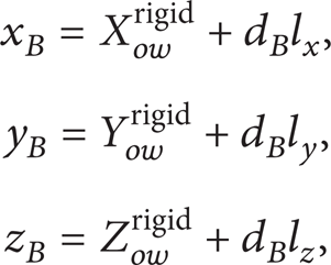
where (X _ow ^rigid, Y _ow ^rigid, Z _ow ^rigid) are described in the coordinate system O₃-X₃Y₃Z₃ defined as a rigid wheelset coordinate system. So the series of the wheel rolling circles can be determined with d _B .

But, for the contact between a flexible wheelset and a pair of rails, due to the axle deformation, as indicated in Figure 5, strictly speaking, d _B is not constant, and the directioncosine components, (l _x , l _y , l _z ), of the central lines of the left and right wheels should be modified. (l _x , l _y , l _z ) in (22) and (23) should be replaced by the direction cosine components, $(l_{(L,R)x},l_{(L,R)y},l_{(L,R)z})$ , of the normal lines at the instant rolling circle centers in O-XYZ; namely, in the calculation of (l_{(L, R)x}, l_{(L, R)y}, l_{(L, R)z}), the rolling and yawing angles (ϕ, ψ) of the wheelset should be replaced by (ϕ_{w(L, R)}, ψ_{w(L, R)}) of the left and right wheels of the flexible wheelset. It should be noted that the normal lines through the instant rolling circle centers are, actually, those through the centers of the nominal rolling circles since the wheels are assumed to be rigid. For the flexible wheelset, the coordinates of the centers of the left and right instant rolling circles should be written as, based on formula (23) and Figure 6,

$\begin{array}{c}{x}_{o_{(L,R)}^{\prime }}=X_{ow}^{\text{rigid}}+\mathrm{\Delta }x+d_{O_{\mathrm{1}}{o}_{(L,R)}^{\prime }}{l}_{(L,R)x},\\ y_{o_{(L,R)}^{\prime }}=Y_{ow}^{\text{rigid}}+\mathrm{\Delta }y+d_{O_{\mathrm{1}}{o}_{(L,R)}^{\prime }}{l}_{(L,R)y},\\ z_{o_{(L,R)}^{\prime }}=Z_{ow}^{\text{rigid}}+\mathrm{\Delta }z+d_{O_{\mathrm{1}}{o}_{(L,R)}^{\prime }}{l}_{(L,R)z},\end{array}$

(24)

where d_{O1o(L, R)′} are the distances between the center O₁ of the flexible wheelset and the centers o_{(L, R)}′ of the left and right instant rolling circles, respectively. And Δx, Δy, and Δz are the increments of the wheelset center translation in the X-, Y-, and Z-directions, respectively. They are caused by the bending deformation of the flexible wheelset. Comparing (23) with (24), for the flexible wheelset, the calculation of the coordinates of the wheelset center O₃ and the instant rolling circle center (x _B , y _B , z _B ) considers the combined effect of the rigid motion and flexible deformation of the wheelset. But its stretching and compressing deformations caused by the axle bending deformation in the axle direction are very small, compared with the axle bending deformation amplitudes. So Δy is neglected. Since the analyzed wheelset is not a powered wheelset, the component along the track of the wheel/rail force is quite small, compared with the vertical component, the bending deformation of the wheelset is very small in a horizontal plane of the track. So Δx caused by the wheelset bending deformation can also be neglected. It should be noted that (X _ow ^rigid, Y _ow ^rigid, Z _ow ^rigid) are obtained through the dynamic analysis using the traditional multibody dynamic model of the vehicle/track, which is introduced in the present paper.

Once the contact circles and the rail top profiles are described in the absolute coordinate system O-XYZ, it will be easy to calculate the minimum distances ΔZ _minL (t) and ΔZ _minR (t) between the wheel treads and rail top surfaces, as well as the coordinates of the wheel/rail contact points. The wheel/rail contact angles can be subsequently calculated with the known coordinates of the wheel/rail contact points and the given wheel/rail profiles.

2.3.3. Wheel/Rail Normal Forces

The vertical instant compressions of wheel/rail at the contact points, δZ _L (t) and δZ _R (t), are written as

$\begin{array}{c}\delta Z_L\left(t\right)=Z_{owL}\left(t\right)-\left(\mathrm{\Delta }{Z}_{\min L}\left(t\right)-\mathrm{\Delta }{Z}_L\left(\mathrm{0}\right)\right)-Z_{\text{irr}L}\left(t\right),\\ \delta Z_R\left(t\right)=Z_{owL}\left(t\right)-\left(\mathrm{\Delta }{Z}_{\min R}\left(t\right)-\mathrm{\Delta }{Z}_R\left(\mathrm{0}\right)\right)-Z_{\text{irr}R}\left(t\right).\end{array}$

(25)

The instant normal compressions, δZ _Lc (t) and δZ _Rc (t), are calculated according to (26) and the contact geometrical relationship shown in Figure 6, and read they as

$\begin{array}{c}\delta Z_{Lc}\left(t\right)=\frac{\delta Z_L\left(t\right)}{\text{cos}({\delta }_L-{\varphi }_{wL})},\\ \delta Z_{Rc}\left(t\right)=\frac{\delta Z_R\left(t\right)}{\text{cos}({\delta }_R+{\varphi }_{wR})}.\end{array}$

(26)

The left and right wheel/rail normal forces $F_{wrn(L,R)}$ are calculated by

$F_{wrn\left(L,R\right)}\left(t\right)=\{\begin{array}{cc}{\left\{\frac{\mathrm{1}}{G}\left[\delta Z_{\left(L,R\right)c}\left(t\right)-\delta Z_{\left(L,R\right)c}\left(\mathrm{0}\right)\right]\right\}}^{\mathrm{3}/\mathrm{2}},\hfill & \delta Z_{\left(L,R\right)c}\left(t\right)\phantom{>-\mathrm{0},}\hfill \\ \hfill & -\delta Z_{\left(L,R\right)c}\left(\mathrm{0}\right)>\mathrm{0},\hfill \\ \mathrm{0},\hfill & \delta Z_{\left(L,R\right)c}\left(t\right)\phantom{\le -\mathrm{0}.}\hfill \\ \hfill & -\delta Z_{\left(L,R\right)c}\left(\mathrm{0}\right)\le \mathrm{0}.\hfill \end{array}$

(27)

Then, the normal force should be decomposed into three components in the X-, Y-, and Z-directions in establishing the motion equations of the wheelset and the rails.

2.3.4. Wheel/Rail Creep Forces and Spin Moments

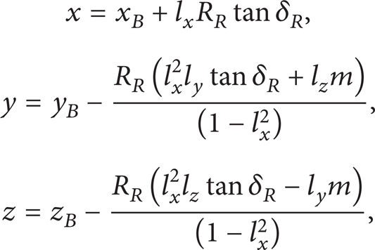
The wheel/rail creep forces are calculated by using the model developed by Shen-Hedrick-Elkins, as described in [18]. In the calculation of each time step, the wheel/rail creepages ξ _x , ξ _y , and ξ _z should be calculated in advance. The existing creepage calculation formulas need to be improved and can be used to calculate the creepages of a flexible wheelset in rolling contact with a pair of rails. The creepages represent the ratios of the relative velocities of the contact surfaces at the contact points to the forward velocities, v_{(L, R)}, of the instant rolling circles of the wheels, as shown in (28). Consider the following:

$\begin{array}{c}{\xi }_{x\left(L,R\right)}=\frac{\mathrm{\Delta }{v}_{\left(L,R\right)x}}{v_{\left(L,R\right)}},\\ {\xi }_{y(L,R)}=\frac{\mathrm{\Delta }{v}_{(L,R)y}}{v_{(L,R)}},\\ {\xi }_{z(L,R)}=\frac{\mathrm{\Delta }{\omega }_{(L,R)z}}{v_{(L,R)}},\end{array}$

(28)

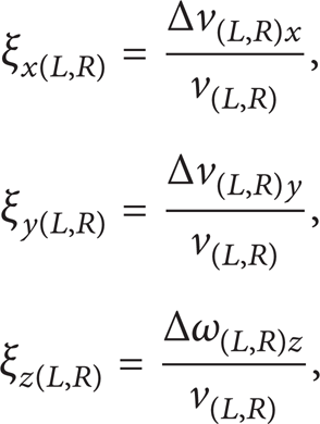
where Δv_{(L, R)x}, Δv_{(L, R)y}, and Δω_{(L, R)z} are, respectively, the relative longitudinal velocity, the relative lateral velocity, and angular velocities. The relative velocities are firstly calculated in the absolute coordinate system and then transformed into the expressions in the local coordinate systems associated with the contact surfaces, which will be discussed in the following.

v_{(L, R)} can be calculated in two ways. The first way is to make a summation of the rigid motion and the flexible deformation of the wheelset, and the other way is to take the derivatives of the coordinates of the centers of the instant rolling circles with respect to time directly. But, actually, the difference between v_{(L, R)} and v is quite small due to the very small effect of the rigid yaw, motion and the bending deformation of the wheelset on the forward speeds, v_{(L, R)}, of the instant rolling circles. So, by using formulas (28), for simplicity, v_{(L, R)} is replaced with v. v is the speed of the vehicle or the nominal forward speed of the wheelset center.

Based on the composite motion theorem of rigid body motion, the absolute velocity v _a of a particle is the resultant vector of the relative velocity v _r and the transport velocity v _e , given in (29). In other words, v _r is the velocity of the moving point, described in the moving coordinate system, and v _e is the velocity of the moving coordinate system relative to the absolute coordinate system. Consider the following:

${\mathbf{v}}_a={\mathbf{v}}_e+{\mathbf{v}}_r.$

(29)

The wheel coordinate systems O_{(L, R)}-X_{(L, R)}Y_{(L, R)}Z_{(L, R)}, as shown in Figure 5, can be regarded as the moving coordinate systems. So the absolute velocities of the left and right contact points O_{(L, R) 1}, respectively, on the left and right wheels, have the following expressions:

${\mathbf{v}}_{wa\left(L,R\right)}={\mathbf{v}}_{we\left(L,R\right)}+{\mathbf{v}}_{wr\left(L,R\right)},$

(30)

where v_{we(L, R)} and v_{wr(L, R)} are, respectively, the transport velocities and the relative velocities. The relative velocities are the velocities of the wheel contact points O_{(L, R) 1} relative to the origins O_{(L, R)} of the moving coordinate systems. The transport velocities v_{we(L, R)} are the velocities of two points in O_{(L, R)}-X_{(L, R)}Y_{(L, R)}Z_{(L, R)}, and these two points coincide with the contact points O_{(L, R) 1}, respectively. So v_{we(L, R)} read as

${\mathbf{v}}_{we\left(L,R\right)}={\mathbf{\omega }}_{\left(L,R\right)}\times {\mathbf{R}}_{O_{(L,R)}{O}_{(L,R)\mathrm{1}}}+{\dot{\mathbf{R}}}_{O{O}_{(L,R)}},$

(31)

where R _{O (L, R) O (L, R) 1} indicate the vectors $\stackrel{⃑}{O_{(L,R)}{O}_{(L,R)\mathrm{1}}}$ . ${\dot{\mathbf{R}}}_{O{O}_{(L,R)}}$ indicate the derivatives of the vectors R _{OO (L, R)} with respect to time. R _{OO (L, R)} are the vectors $\stackrel{⃑}{O{O}_{(L,R)}}$ . ${\dot{\mathbf{R}}}_{O{O}_{(L,R)}}$ represent the translational velocities of the centers of the nominal rolling circles of the left and right wheels, described in the absolute coordinate system. ω_{(L, R)} are determined by the angular velocity vectors of the left and right wheels, ${\dot{\psi }}_{w(L,R)}$ and ${\dot{\varphi }}_{w(L,R)}$ , as indicated in (32). It is noted that ω_{(L, R)} is just the rotation of the transport coordinate systems, O_{(L, R)}-X_{(L, R)}Y_{(L, R)}Z_{(L, R)}, relative to the absolute coordinate system O-XYZ, as shown in Figure 5. Consider the following:

$\begin{array}{c}{\mathbf{\omega }}_{\left(L,R\right)}={\left[\begin{array}{c}{\dot{\varphi }}_{w\left(L,R\right)}\\ \mathrm{0}\\ {\dot{\psi }}_{w\left(L,R\right)}\end{array}\right]}^T\left\{\begin{array}{c}\mathbf{i}\\ \mathbf{j}\\ \mathbf{k}\end{array}\right\},\\ {\mathbf{R}}_{O_{(L,R)}{O}_{(L,R)1}}={\left[\begin{array}{c}{\dot{R}}_{(L,R)x}^{\prime }\\ {\dot{R}}_{(L,R)y}^{\prime }\\ {\dot{R}}_{(L,R)z}^{\prime }\end{array}\right]}^T\left\{\begin{array}{c}{\mathbf{i}}_{\left(L,R\right)}\\ {\mathbf{j}}_{\left(L,R\right)}\\ {\mathbf{k}}_{\left(L,R\right)}\end{array}\right\}.\end{array}$

(32)

It should also be noted that ω_{(L, R)} do not include the rolling (ω₀) of the rigid wheelset over the track and neglect the rolling angular velocities of the wheels due to the twisting deformation of the wheelset, which produce the longitudinal creepages. The relative velocities v_{wr(L, R)} are the velocities of the left and right contact points described in the local coordinate systems O_{(L, R)}-X_{(L, R)}Y_{(L, R)}Z_{(L, R)}, due to the rolling of the wheelset over the two rails. They are written as

${\mathbf{v}}_{wr\left(L,R\right)}={\mathbf{\omega }}_{\left(L,R\right)}^{\prime }\times {\mathbf{R}}_{O_{(L,R)}{O}_{(L,R)\mathrm{1}}},$

(33)

where

${\mathbf{\omega }}_{\left(L,R\right)}^{\prime }={\left[\begin{array}{c}\mathrm{0}\\ -{\omega }_{\mathrm{0}}\\ \mathrm{0}\end{array}\right]}^T\left\{\begin{array}{c}{\mathbf{i}}_{(L,R)}\\ {\mathbf{j}}_{(L,R)}\\ {\mathbf{k}}_{(L,R)}\end{array}\right\}.$

(34)

Equation (34) is expressed in the local coordinate systems O_{(L, R)}-X_{(L, R)}Y_{(L, R)}Z_{(L, R)}.

Substituting (31) and (33) into (30), the equation could be deduced as follows:

${\mathbf{v}}_{wa\left(L,R\right)}={\mathbf{v}}_{we\left(L,R\right)}+{\mathbf{v}}_{wr\left(L,R\right)}={\dot{\mathbf{R}}}_{O{O}_{\left(L,R\right)}}+{\mathbf{\omega }}_{\left(L,R\right)}\times {\mathbf{R}}_{O_{\left(L,R\right)}{O}_{\left(L,R\right)\mathrm{1}}}+{\mathbf{\omega }}_{\left(L,R\right)}^{\prime }\times {\mathbf{R}}_{O_{\left(L,R\right)}{O}_{\left(L,R\right)\mathrm{1}}}.$

(35)

It should be noted that v_{wr(L, R)} should be transformed into the expression in absolute coordinate system O-XYZ through using transformation matrices A_{w(L, R)}, as indicated in (16), before being added to the calculation.

The absolute velocities of the contact points on the left and right rails are written as

${\mathbf{v}}_{\text{rail}(L,R)}={\left[\begin{array}{c}{\dot{X}}_{r(L,R)}\\ {\dot{Y}}_{r(L,R)}\\ {\dot{Z}}_{r(L,R)}\end{array}\right]}^T\left\{\begin{array}{c}\mathbf{i}\\ \mathbf{j}\\ \mathbf{k}\end{array}\right\}+{\left[\begin{array}{c}\delta {\dot{X}}_{r(L,R)}\\ \delta {\dot{Y}}_{r(L,R)}\\ \delta {\dot{Z}}_{r(L,R)}\end{array}\right]}^T\left\{\begin{array}{c}\mathbf{i}\\ \mathbf{j}\\ \mathbf{k}\end{array}\right\},$

(36)

where ${\dot{Y}}_{r(L,R)}$ and ${\dot{Z}}_{r(L,R)}$ are, respectively, the lateral and vertical velocities of the left and right rail cross-sections and $\delta {\dot{Y}}_{r(L,R)}$ and $\delta {\dot{Z}}_{r(L,R)}$ are, respectively, the rates of changes of the lateral and vertical irregularities on the left and right railheads.

Using (35) and (36), the velocity differences Δv_{(L, R)} between the contact surfaces of the wheels and the rails can be written as

$\mathrm{\Delta }{\mathbf{v}}_{(L,R)}={\mathbf{v}}_{wa\left(L,R\right)}-{\mathbf{v}}_{\text{rail}\left(L,R\right)}={\left[\begin{array}{c}\mathrm{\Delta }{v}_{x\left(L,R\right)}\\ \mathrm{\Delta }{v}_{y\left(L,R\right)}\\ \mathrm{\Delta }{v}_{z\left(L,R\right)}\end{array}\right]}^T\left\{\begin{array}{c}\mathbf{i}\\ \mathbf{j}\\ \mathbf{k}\end{array}\right\}.$

(37)

The velocity differences Δv_{(L, R)}, are expressed in the absolute coordinate system, shown in (37), and then need to be transformed into the expressions in the local coordinate systems O_{(L, R) 1}-X_{(L, R) 1}Y_{(L, R) 1}Z_{(L, R) 1} through (18).

Then, plugging (18) into (37), the velocity differences are

$\mathrm{\Delta }{\mathbf{v}}_{\left(L,R\right)}={\left[\begin{array}{c}\mathrm{\Delta }{v}_{x\left(L,R\right)}\\ \mathrm{\Delta }{v}_{y\left(L,R\right)}\\ \mathrm{\Delta }{v}_{z\left(L,R\right)}\end{array}\right]}^T{{\mathbf{A}}_{\left(L,R\right)\mathrm{1}}}^{-\mathrm{1}}\left\{\begin{array}{c}{\mathbf{i}}_{\left(L,R\right)\mathrm{1}}\\ {\mathbf{j}}_{\left(L,R\right)\mathrm{1}}\\ {\mathbf{k}}_{\left(L,R\right)\mathrm{1}}\end{array}\right\}={\left[\begin{array}{c}\mathrm{\Delta }{v}_{\left(L,R\right)x}^{\prime }\\ \mathrm{\Delta }{v}_{\left(L,R\right)y}^{\prime }\\ \mathrm{\Delta }{v}_{\left(L,R\right)z}^{\prime }\end{array}\right]}^T\left\{\begin{array}{c}{\mathbf{i}}_{\left(L,R\right)\mathrm{1}}\\ {\mathbf{j}}_{\left(L,R\right)\mathrm{1}}\\ {\mathbf{k}}_{\left(L,R\right)\mathrm{1}}\end{array}\right\}.$

(38)

Equation (38) is plugged into (28) to calculate the lateral and longitudinal creepages. The calculation of the spin creepages by using the third formula in (28) neglects the effect of the wheelset axle bending since its effect on the spin creepages is quite small.

3. Results and Discussions

In order to verify the present model considering the effect of the first-order bending modes of the wheelset in the two planes mentioned above on the rolling contact behavior, a harmonic track irregularity with fixed wavelength of 1.18 m is used. The excitation frequency of the irregularity is 117 Hz at the speed of 500 km/h, which is exactly equal to the resonance frequency of the wheelset first-order bending mode. The fluctuating amplitude of the irregularity is 0.05 mm. The calculation cases include the speeds of 200 km/h, 300 km/h, 400 km/h, and 500 km/h. The parameters used in the calculation are listed in Table 1 [20].

In Figure 7, the right vertical axis denotes the difference (DIFF) between the normal forces calculated by the models of the rigid (RW) and flexible (EW) wheelsets. The lines of DIFF in Figure 7 are obtained by subtracting the lines of RW from the corresponding lines of EW. The numerical computation benefits from fast double precision. Figure 7 shows that the amplitudes of the total vertical wheel/rail forces increase with the speed increase, as indicated by the red and blue broken lines. The amplitude of the normal force difference denoted by DIFF, that is, the normal force variation caused by the first-order wheelset bending deformation, is about 0.2 N when the speed is less than 500 km/h, as shown in Figures 7(a), 7(b), and 7(c). In the case of 500 km/h, as shown in Figure 7(d), the maximum amplitude of the difference reaches about 1.2 N, which is 6 times larger than those of the cases of Figures 7(a), 7(b), and 7(c). This is caused by the excited resonance of first-order bending mode. An increase in the wheel/rail normal force caused by the first-order bending resonance is quite small, compared with the static wheel/rail forces. But such a small difference of the force applied on wheels at a fixed frequency could cause a polygonal wear on high-speed wheels in a long-time service. For instance, now the high-speed vehicles in service widely use the wheelsets with diameters in the range of 840 mm–920 mm, and the operating speed of the high-speed trains is 300 km/h. Large amounts of wheel tread roughness measured from the sites show that the trilateral wear on the wheels is very common due to the wheelset first-order bending resonance excited probably.

Figure 7:

Wheel/rail vertical forces at the speeds of (a) 200 km/h, (b) 300 km/h, (c) 400 km/h, and (d) 500 km/h. RW and EW denote the cases of the rigid wheelset and the elastic wheelset, respectively, and DIFF illustrates the difference between the analysis results of the rigid and the elastic wheelsets.

Figure 8 indicates the PSDs (power spectral densities) of the vertical forces, corresponding to those analyzed in time domain in Figure 7. The frequencies of the dominant vibration components (at peaks) in Figure 8 are the excitation frequencies of the harmonic track irregularity, which are, respectively, 46 Hz, 69 Hz, 92 Hz and 117 Hz at the speeds of 200 km/h, 300 km/h, 400 km/h, and 500 km/h. This indicates that track irregularity plays a dominant role in the influence on wheel/rail vertical force. In other words, the influence of the wheelset flexibility is not significant if the resonance frequency of the first-order bending mode is far away from the passing irregularity frequency. The lines of DIFF illustrate the PSDs of the differences between the vertical forces applied on the rigid and flexible wheelsets. In Figures 7(a), 7(b), and 7(c), three frequency components dominate the PSDs of the force differences. The first is that f₁ = 31 Hz, which is the natural frequency of the wheel-rail contact system independent of the operating speed. The second is the passing harmonic track irregularity frequency, f₂ that is equal to, respectively, 46 Hz, 69 Hz, 92 Hz and 117 Hz, corresponding to the speeds of 200 km/h, 300 km/h, 400 km/h and 500 km/h. The third is the first-order bending resonance frequency, f₃. At the speed of 500 km/h, the peak value, as seen in Figure 8(d), is about two orders of magnitude larger than the values at the frequency of 117 Hz at the other three speeds. So the difference in the dynamic behavior of the rigid and flexible wheelsets has been clearly understood.

Figure 8:

The PSDs of the vertical wheel/rail forces at the speeds of (a) 200 km/h, (b) 300 km/h, (c) 400 km/h, and (d) 500 km/h: f₁ = 31 Hz, f₂ = 46 Hz in (a), f₂ = 69 Hz in (b), f₂ = 92 Hz in (c), f₂ = 117 Hz in (d), and f₃ = 117 Hz.

The differences of the lateral wheel/rail forces and their PSDs have almost the same features. So the discussion on them is omitted in this paper.

The excited wheelset bending mode makes a contribution to the wheel/rail interaction to some extent, as known from the above analysis on the wheel/rail forces. The first-order bending resonance causes the oscillations of the wheel/rail contact points and the relative velocity of the wheel/rail contact surfaces. Figure 9 shows the changes of contact points on the rigid and flexible wheelsets with the travelling distance. In Figure 8, the vertical axis represents the coordinates of the wheel contact points in the direction of Y_{(L, R)} axis of the local coordinate systems O_{(L, R)}-X_{(L, R)}Y_{(L, R)}Z_{(L, R)}. The black heavy lines indicate the traces of the contact points on the rigid wheelset and the fine red lines denote those on the flexile wheelset, which are, respectively, indicated by RW and EW. The contact points on the rigid wheelset are closer to the nominal rolling circles, and the contact points on the flexible wheelset move toward their corresponding field sides due to the bending deformation. The first-order bending resonance of the wheelset in the plane perpendicular to the track level causes the opposite rolling angles of the left and right wheels, which are nearly symmetrical about the wheelset centre. This mode shape is similar to the downward bending deformation of the wheelset axis, as shown in Figure 3. With the increase of the speed the passing irregularity frequency gradually approaches the wheelset resonance frequency of the first-order bending mode, so that the trace of the contact points oscillates more and more seriously. When the vehicle speeds up to 500 km/h, as displayed in Figure 9(d), the first-order bending resonance of the wheelset occurs and the left and right contact points on the elastic wheelset fiercely fluctuate around the traces of the contact points on the rigid wheelset. The fluctuating amplitude reaches 0.1 μm, and is five times larger than those at the speeds of 200 km/h 300 km/h and 400 km/h.

Figure 9:

Lateral coordinates of contact points on wheel treads in associated coordinate systems at the speeds and of (a) 200 km/h, (b) 300 km/h, (c) 400 km/h, and (d) 500 km/h.

It is very interesting that the contact point traces of the rigid wheelset do not present the obvious oscillation at the passing frequency of the harmonic regularity excitation, as indicated by the black lines of RW. However, the RW lines show the position oscillations of the contact points on the rigid wheelset at a low-frequency about 22 Hz. The frequency is probably the natural frequency of the bogie in the lateral direction. The resonance of the bogie is caused by the harmonic track irregularity. When the speed is 400 km/h, the low frequency oscillation reaches the largest, as indicated in Figure 9(c), and when the speed is 500 km/h, the oscillation disappears, as indicated by the coarse black lines in Figure 9(d). The further discussion on dynamic behavior of the bogie does not belong to the task of this paper.

The above analysis shows the evident impact of the wheelset bending deformation on the contact points. The wheel/rail contact forces rely on not only the contact point positions but also the relative speeds of the contact surfaces represented by the creepages. There is a small difference between the creepages calculated with the models of the elastic and rigid wheelsets, as indicated in Figure 10.

Figure 10:

Lateral creepage at the speed of 500 km/h.

As well known, rail corrugation and wheel polygonization are mainly related to the sensitive resonances of the wheel/rail system [1, 21, 22]. In order to verify that the first-order bending resonance of the wheelset is active and find the sensitive resonance frequencies of the wheel/rail systems, the present model of the high-speed vehicle coupled with the track is used to analyze the dynamic behaviour of the wheel/rail systems under a white-noise excitation and at different speeds. The analyzed frequency range is from 0 to 500 Hz and the operation speed is from 200 km/h to 400 km/h. Figure 11 shows the wheel/rail force responses analyzed in frequency-domain. Figures 11(a) and 11(b) illustrate the linear spectra of the lateral and vertical wheel/rail forces of the rigid wheelset, respectively, and Figures 11(c) and 11(d) indicate the corresponding results of the flexible wheelset. In Figure 11(b), f₀ indicates the resonance frequency of the wheel/rail system, as mentioned above. It is about 31 Hz, and independent of the operation speed. In Figures 11(a) and 11(b), f _s is the passing frequency of the sleepers and 2f _s is the twice passing frequency of the sleepers or called harmonic frequency due to the excitation of the multisleepers with an equal pitch between the neighboring sleepers. In Figures 11(c) and 11(d), f_m1 denotes the bending resonance frequency of the wheelset. f_m1 equals 117 Hz, and it is evident that the resonance frequency is independent of the vehicle speed. In all the figures of Figure 11, f _t always appears at about 380 Hz. It is one of the resonance frequencies of the system consisting of the track and the bogie of the vehicle. It will be further analyzed in the following.

Figure 11:

Wheel/rail force amplitudes in frequency domain at different speeds and under a white-noise roughness excitation: (a) the lateral forces on the rigid wheelset; (b) the vertical forces on the rigid wheelset; (c) the lateral forces on the flexible wheelset; and (d) the vertical forces on the flexible wheelset.

Carefully making a comparison of Figures 11(a), 11(b), 11(c), and 11(d) shows the interesting results, in which one should carefully pay attention to the vertical coordinate scales of the figures. Under the present excitation of the white-noise, the wheel/rail force response has high peaks at the passing frequencies of the sleepers, or the wheel/rail force response to the excitation of the periodically discrete sleepers is clearly characterized by using the existing model of the coupling vehicle/track without considering the effect of the first-order bending resonance of wheelset, as indicated in Figures 11(a) and 11(b). But the wheel/rail force response has very low peaks at the passing frequencies of the sleepers in Figures 11(c) and 11(d) in which the results are calculated by using the model considering the effect of the flexible wheelset. Actually, the wheel/rail force response to the excitation of the periodically discrete sleepers is overwhelmed by the responses at the other resonance frequencies. So the first-order bending resonance of the wheelset plays a dominant role in the wheel/rail force response under the present excitation of the white-noise and in the analyzed speed range.

The peaks at f _t ≈ 380 Hz are always remarkable in the results obtained by the two models, or the vibration at about 380 Hz always makes a great contribution to the wheel/rail force response. This is because f _t is the resonance frequency of the track including the effect of the sprung mass and the bogie frame of the vehicle, and in the employed two models the track modelling is the same. In order to find the mode shape of the track resonance, a finite element model for the track with a bogie is developed and used to calculate the resonance frequencies and the corresponding mode shapes of them. In Figure 12, the two figures indicate the mode shapes of the track with a bogie, the corresponding frequencies of which are, respectively, 374 Hz and 390 Hz. They are close to 380 Hz.

Figure 12:

Track mode shapes with resonance frequencies near 380 Hz.

4. Conclusions

This paper presents a new vehicle/track coupling dynamics model considering the effect of the first-order bending resonance of the flexible wheelset. A new wheel/rail contact geometry model is derived in detail and considers the interaction of a flexible wheelset and a pair of rails. So the existing coupling dynamics model of railway vehicle/track is further improved. In order to verify the new model and clarify the influence of the first-order bending resonance of the flexible wheelset on the wheel/rail contact behavior, the new and existing models are used to analyze the difference of the wheel/rail contact behavior under the excitation of a harmonic track irregularity with a fixed wavelength and a white-noise at different operating speeds. The results calculated by the two models are compared to understand the effect of the wheelset first-order bending on the rolling contact behavior of the wheel/rail system. The conclusions are given as follows.

1. In the analysis cases that indicate the different operating speeds and a harmonic irregularity and white-noise excitations, the first-order bending mode of the wheelset in service can be excited easily. When the passing irregularity frequency equals the natural frequency of the first-order bending mode of wheelset, the resonance of the wheel/rail systems occurs. In such a situation, the wheelset bending has a great influence on the wheel/rail rolling contact behavior.

2. When the first-order bending mode in the vertical plane is excited at the speed of 500 km/h, the wheel/rail forces and contact points oscillate more seriously than those at the other speeds at the first-order bending resonance frequency. Besides, the resonance easily occurs between the flexibility wheelset and the rails when the passing frequency of the track irregularity excitation is equal or close to the wheelset bending resonance frequency at any speed. Though the numeric differences between the dynamic responses of the rigid and flexible wheelsets are small, they could contribute to the development of the polygonal wear on the wheel treads after a long-time service of the wheelset.

3. Developing the coupling dynamics model of railway vehicle and track considering the effect of structural flexibility of the key parts is a complex subject. The present work is just at a preliminary stage. The next step will be to consider modeling the high-order bending resonances of wheelset, wheel flexibility and powered wheelset flexibility in the wheel/rail rolling contact model.