W-LEACH Based Dynamic Adaptive Data Aggregation Algorithm for Wireless Sensor Networks

Abstract

We consider the problem of data aggregation for nonuniform and evolving wireless sensor networks. We introduce a new data aggregation algorithm that is able to run on uniform, non-uniform, and evolving networks while maintaining the data accuracy. In addition, the algorithm is able to handle sudden bursts in the underlying data by recording the data in the area of interest for the whole event duration. Experimental results on real and synthetic data show that the algorithm performs well in terms of extending the lifetime of the network, maintaining the original distribution of the sensors as long as possible, maintaining the accuracy of the sensed data, and being able to detect and handle sudden bursts of data.

1. Introduction

Wireless sensor networks (WSNs) are wireless networks that consist of spatially distributed wireless sensors; small battery-powered devices that are distributed among geographical areas to continuously collect data. Examples of WSN-based applications include environmental monitoring, flood detection, and home automation.

Wireless sensors have limited capabilities since they are battery powered. They have limited lifetimes and short communication ranges. The collected data is then sent to central units (base stations) for processing, analysis, and decision taking. Examples of the data that can be collected include temperature, humidity, light conditions, and seismic activities. This data can be used to detect certain events and to trigger activities.

Designing a reliable WSN requires many efficient methods in routing, data aggregation, and localization. In this work, we only consider the problem of data aggregation to improve the network lifetime. Data aggregation algorithms for WSNs aim to reduce the size and amount of data transfer and, therefore, process less data records by defining the techniques for gathering data from sensors and forwarding them to base stations. These techniques include the decisions of which data records to be sent and what is the best time to send them.

Since aggregation algorithms can decide not to send some data records at certain time periods in order to save battery power, the aggregated data may not reflect the actual recorded values. This might affect the accuracy of the decisions that are taken by the system. Data accuracy of the aggregated data is, therefore, a major concern in the field of data aggregation algorithms to ensure accurate system decisions.

There are many data aggregation methods that are proposed in the literature, such as LEACH, DD, FEDA, TAG, OCABTR, CLUDDA, and SUMAC [1–15]. Many of the existing aggregation algorithms for WSNs are designed to work with cluster-based routing algorithms [1–7, 10, 13–15], while some others are based on other ways of routing [8, 9, 11, 12] such as direct connection between sensors and the base station.

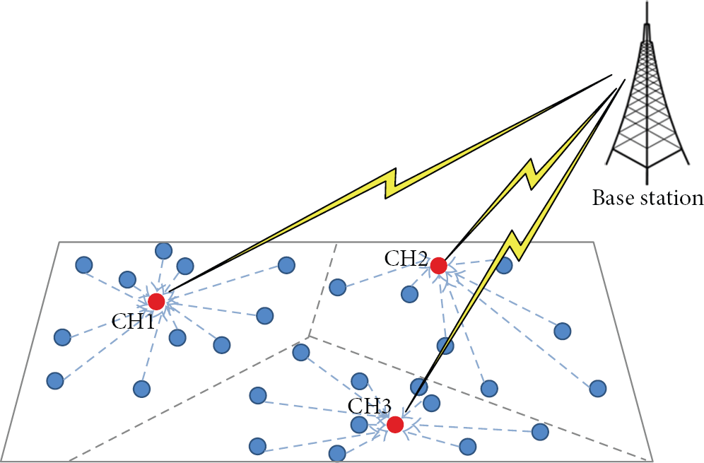
We only consider the cluster-based routing algorithms by which nearby sensors are grouped together to form a number of clusters. Each cluster is represented by one sensor called cluster head (CH). CHs collect data records from other sensors in their clusters and then send the aggregated data to the base station. This technique saves energy, since not all sensors are required to communicate with the base station.

One well-known cluster-based data aggregation algorithm for WSN is Low Energy Adaptive Clustering Hierarchy Aggregation (LEACH) algorithm by Heinzelman et al. [7]. LEACH has recorded good results in increasing the network life time by saving the total energy of sensors.

WSNs can have nonuniform distribution for sensors. Networks for agricultural application, for example, may suffer from being nonuniform according to erosion, even if they started with a uniform distribution. Applications that are based on mobile sensors, such as in traffic applications that require sensors to be attached to vehicles, also form a nonuniform distribution. Uniform networks can also experience some sensors that die with time when their energy is consumed, which may lead to a nonuniform distribution at some point. WSNs can, hence, be networks of evolving nature since the distribution of the sensors in the networks of the above example may change with time.

The values of the sensed data can, also, change in distributions. They can either gradually change or have sudden bursts. Sudden changes of values in specific sensors of the network can happen according to the occurrence of any event, for example, nature hazards in field applications or sudden medical disorder in health application. Such changes would be of interest to capture their data values in order to ensure that no important events in the sensed field are lost.

The main contribution of this paper is to introduce a data aggregation algorithm for WSNs that aims to reduce the energy consumption of sensors and, therefore, increase the network life time without critically affecting the data accuracy. The algorithm is intricate, so we introduce its explanation in three phases. The first phase presents a new algorithm, namely, Weighted Low Energy Aggregation Clustering Hierarchy (W-LEACH) [1]. W-LEACH directly extends LEACH-C [6] to introduce the concept of weighted sensors that is used to decide which sensors are chosen to be cluster heads and which sensors are chosen to send data at certain rounds. Weights are assigned to sensors based on their remaining energy as well as their density; a newly developed measure that defines the percentage of its surrounding sensors to the total number of sensors.

The second phase [2] adds more to the technical aspects of the algorithm to achieve longer network lifetime. We name the algorithm in this phase as Dynamic W-LEACH since it adds a dynamic nature to one important parameter of W-LEACH. The algorithm in this phase is also tested on networks with evolving nature.

The third phase considers the data accuracy when applying Dynamic W-LEACH on nonuniform WSNs, to show that the algorithm does not seriously affect the general accuracy of the collected data. This is shown by applying our algorithm on real data and recording the accuracy level. The algorithm is, then, modified to reach a level of adaptivity, so that it can handle any sudden bursts in the underlying data values in order to continuously make sure that data in the areas of interest is captured.

We simulate our algorithm and compare the network life time and accuracy to LEACH. We use real data as well as synthetic data for our tests. Experimental results show that our algorithm performs well when applied on both nonuniform and evolving networks. It increases the network life-time while not severely affecting the accuracy of the results. The results also demonstrate the adaptivity of the algorithm by being able to capture the events of interest.

The remainder of the paper is organized as follows. Section 2 states some background and related work. Section 3 proposes the W-LEACH algorithm. Section 4 further extends W-LEACH to introduce the Dynamic W-LEACH algorithm. Section 5 improves some technical aspects of Dynamic W-LEACH in order for it to be adaptive to sudden changes in data. Section 6 explains the implementation and experimental settings. Section 7 states the discussion and results. Finally, Section 8 draws our conclusions.

2. Background

2.1. LEACH Algorithm

Low Energy Adaptive Clustering Hierarchy Aggregation (LEACH) algorithm by Heinzelman et al. [7] is a data aggregation algorithm based on cluster routing. The algorithm works in rounds such that each round has two phases, namely, a setup phase and a steady state phase.

In the setup phase, $p\%$ of n sensors are uniformly randomly chosen to be cluster heads (CHs) based on a threshold

$$\begin{array}{cc}& T\left(n\right)=\{\begin{array}{cc}\frac{p}{\mathrm{1}-p\left(t\mathrm{mod}\left(\mathrm{1}/p\right)\right)},\hfill & \text{if}\mathrm{\hspace{0.17em}\hspace{0.17em}}n\in G,\hfill \\ \mathrm{0},\hfill & \text{otherwise},\hfill \end{array}\end{array}$$

(1)

where p is the desired number of CHs, t is the current round, and G is the set of nodes that have not been CHs in the last $\mathrm{1}/p$ rounds. This ensures that a sensor that is chosen to be CH is not chosen in the next rounds until all other sensors in the network become CHs. This feature leads to fair energy consumption, hence, the network lifetime is increased. The algorithm does not consider nonuniform networks since the CHs are chosen uniformly randomly. After all CHs are chosen, clusters are dynamically defined such that each non-CH becomes a member of the cluster with the nearest CH.

In the steady state phase, each CH collects data from all sensors in its cluster based on Time Division Multiple Access (TDMA). CHs, then, compress the collected data and send it to the base station. See Figure 1.

Figure 1

LEACH aggregation algorithm.

3. Weighted Low Energy Adaptive Clustering Hierarchy Aggregation (W-LEACH)

Weighted Low Energy Adaptive Clustering Hierarchy Aggregation (W-LEACH), is a centralized data aggregation algorithm [1]. As in LEACH, W-LEACH consists of a setup phase and a steady state phase. In the setup phase, W-LEACH first calculates a weight value, $w_i$ , and assigns it to each sensor $s_i$ . We modify the definition of p to be the percentage of the maximum number of CHs instead of the actual number of CHs as it is defined in the original LEACH. A maximum of $p\%$ of alive sensors are, then, selected to be CHs based on the calculated weights, such that the higher the weights the better the chance for them to be CHs. Note that unlike LEACH, W-LEACH does not take into consideration whether or not this sensor was a CH for previous near rounds. After all CHs are chosen, clusters are formed such that each sensor is assigned to its nearest CH.

The weights are calculated as

$$\begin{array}{cc}& w_i=\{\begin{array}{cc}{e}_i*d_i,\hfill & \text{if}\hspace{0.17em}\hspace{0.17em}{d}_i>d_{\text{thresh}},\hfill \\ d_i,\hfill & \text{otherwise},\hfill \end{array}\end{array}$$

(2)

where $d_i=(\mathrm{1}$ + number of alive sensors in range $\mathrm{\hspace{0.17em}\hspace{0.17em}}r)/n$ is the density of the sensor $s_i$ , r is the range that is reachable by sensor $s_i$ , $e_i$ is the remaining energy in sensor $s_i$ , and $d_{\text{thresh}}$ is a density threshold to define the set of sensors in very low density areas. We define $d_{\text{thresh}}=r_{\text{thresh}}/n$ so that it changes with the number of alive sensors n, where $r_{\text{thresh}}$ is the number of sensors that defines the low density areas and its application specific. In this work, we choose $r_{\text{thresh}}$ to be 1. $d_{\text{thresh}}$ , therefore, substitutes to the value of $\mathrm{1}/n$ . Note that because the maximum value of $d_i$ is 1 and the maximum value of $e_i$ is $\mathrm{1}J$ (as suggested by LEACH), then the term $e_i*d_i$ can not exceed the value of 1, and the higher the value of $e_i$ and/or $d_i$ , the higher the weight $w_i$ .

In the steady state phase, W-LEACH chooses a number of sensors in each cluster to send data to their CHs based on a fixed percentage $x=\mathrm{50}\%$ , unlike LEACH, which requires that each CH collects data from all sensors in its cluster. The candidates for sending data to CHs are also chosen based on their weights, such that sensors with less weights are better candidates to send data to their CHs to make sure that the areas with low densities and far from their CHs are covered. Sensors with densities ≤ $d_{\text{thresh}}$ might, therefore, be chosen more frequently because of their low weights, and, thus, their life time may be shortened. To solve this problem, W-LEACH requires that sensors in these areas send data with some probability $ps$ , such that in each round t, $x\%$ sensors are chosen; then if any of these chosen sensors has the value of $d_i\le d_{\text{thresh}}$ , then it does not send data to the CH unless it satisfies a probability $ps$ , which is an application specific parameter and can be chosen empirically. Details of W-LEACH algorithm can be found in the paper by Abdulsalam and Kamel [1].

4. Dynamic W-LEACH: W-LEACH with Variable Percentage of Sending Sensors

We modify W-LEACH to further minimize the overall energy consumption in the network. We define a new metric, namely, CH-density ( $d_{\text{CH}}$ ), to represent the density of clusters. CH-density is calculated as the ratio of the number of alive sensors in a cluster i to the the total number of alive sensors as follows:

$$\begin{array}{cc}& d_{{\text{CH}}_i}=\frac{\left(\text{number}\mathrm{\hspace{0.17em}\hspace{0.17em}}\text{of}\mathrm{\hspace{0.17em}\hspace{0.17em}}\text{alive}\mathrm{\hspace{0.17em}\hspace{0.17em}}\text{sensors}\mathrm{\hspace{0.17em}\hspace{0.17em}}\text{in}\mathrm{\hspace{0.17em}\hspace{0.17em}}{\text{cluster}}_i\right)}{\left(\text{total}\mathrm{\hspace{0.17em}\hspace{0.17em}}\text{number}\mathrm{\hspace{0.17em}\hspace{0.17em}}\text{of}\mathrm{\hspace{0.17em}\hspace{0.17em}}\text{alive}\mathrm{\hspace{0.17em}\hspace{0.17em}}\text{sensors}\right)}.\end{array}$$

(3)

We then use this metric to dynamically adjust x, the number of sending sensors for each cluster, such that clusters with more sensors assigned to them (higher CH-density) have less percentage than clusters with less sensors (lower CH-density). This is justified as follows: for clusters with high $d_{\text{CH}}$ , the percentage of sending sensors could be safely decreased and yet result in a reasonable number of sending sensors, while for clusters with low $d_{\text{CH}}$ , the percentage is required to be increased in order to reach a reasonable number of sending sensors.

The percentage of sensors to send data in W-LEACH x is, therefore, redefined as

$$\begin{array}{cc}& x_{\text{dynamic}}=\{\begin{array}{cc}\mathrm{0.1},\hfill & \text{if}\hspace{0.17em}\hspace{0.17em}\mathrm{0.0}{\mathrm{1}}^{d_{\text{CH}}}<\mathrm{0.1},\hfill \\ \mathrm{0.5},\hfill & \text{if}\hspace{0.17em}\hspace{0.17em}\mathrm{0.0}{\mathrm{1}}^{d_{\text{CH}}}>\mathrm{0.5},\hfill \\ \mathrm{0.0}{\mathrm{1}}^{d_{\text{CH}}},\hfill & \text{otherwise}.\hfill \end{array}\end{array}$$

(4)

As it can be seen from the above equation, $x_{\text{dynamic}}$ varies from 0.1 to 0.5 (10% to 50%). Note that when $x_{\text{dynamic}}=\mathrm{0.5}$ , then the algorithm acts as the original W-LEACH that is presented in Section 3. Since our target is to reduce the number of sending sensors whenever possible rather than increasing them, we set the maximum limit in the above equation to be as the original W-LEACH. The minimum limit is application specific, and we choose it to be 10% to ensure that the number of chosen sensors for big clusters at any time is not very low, and therefore data is not lost.

It can be also shown from the above equation that $x_{\text{dynamic}}$ is inversely proportional to the value of $d_{\text{CH}}$ . That is, the more sensors a cluster has, the less percentage of its sensors is chosen to send data. Solving the above equation for $d_{\text{CH}}$ , the minimum $x_{\text{dynamic}}=\mathrm{0.1}$ is reached for clusters with $d_{\text{CH}}\ge \mathrm{0.5}$ , which are clusters with 50% or more of the alive sensors in the network that are assigned to them, whereas the maximum $x_{\text{dynamic}}=\mathrm{0.5}$ is reached for clusters with $d_{\text{CH}}\le \mathrm{0.15}$ , which are clusters with 15% or less of the alive sensors in the network that are assigned to them.

5. Adaptivity Feature for Dynamic W-LEACH

We further modify Dynamic W-LEACH in order to handle sudden bursts in the underlying values of the data. Changes in data may appear according to sudden events in the sensed field. Handling such sudden events is based on the actual values of the sensed data. The algorithm should, therefore, keep track of the values of the data for each sensor independently.

For each sensor $s_i$ in the network, at a specific round t, the change in values of the sensed data affects the weight $w_i$ of this sensor. The more serious the change is, the more the weight is reduced to have a better chance to be selected by the algorithm to send data to its CH for this specific round. Recall that from previous explanation of W-LEACH in Section 3, the sensors that have less weights are better candidates to be chosen to send data to their cluster heads. Note that the number of sending sensors in each cluster is not affected by this improvement. This phase only highlights the area of interest so that the algorithm is more attracted to choose sensors in the area of interest to send data to their cluster heads in order to reflect the changes.

The algorithm keeps track of the change in values of sensor $s_i$ , such that for each round t, the accumulated average $v_{i_{\text{avg}}}(t)$ is calculated as the average of values seen so far. The difference between the current recorded value and the average $\mathrm{\Delta }{v}_i(t)=v_i(t)-v_{i_{\text{avg}}}(t)$ is also calculated. Suppose that sensor $s_i$ is located in cluster $c_k$ at round t. We define $\mathrm{\Delta }{v}_{c_{k_{\max }}}(t)=\max ({v_i(t)|}_{c_k})$ . The ratio of the difference $\mathrm{\Delta }{v}_i(t)$ to the maximum recorded difference in cluster $c_k$ at round $t(\mathrm{\Delta }{v}_{c_{k_{\max }}}(t))$ : $V_i(t)=\mathrm{\Delta }{v}_i(t)/\mathrm{\Delta }{v}_{c_{k_{\max }}}(t)$ is what affects the weight. The higher the ratio $V_i(t)$ , the lower the weight.

The weight formula is accordingly modified as follows:

$$\begin{array}{cc}& w_i=\{\begin{array}{cc}{e}_i*d_i^{\mathrm{1}+V_i},\hfill & \text{if}\hspace{0.17em}\hspace{0.17em}{d}_i>d_{\text{thresh}},\hfill \\ d_i^{\mathrm{1}+V_i},\hfill & \text{otherwise}.\hfill \end{array}\end{array}$$

(5)

The modification is a plausible solution to reflect the required constraints as follows:

• (i)

  for no changes in values, the density is not affected as $V_i$ is zero, and therefore the weight remains the same.

• (ii)

  as changes occur, the value of $V_i$ starts to affect the weight, such that a larger value of $V_i$ means a more serious change, therefore, a higher value of the power and a less overall value of the weight since the density is a fraction; $\mathrm{0}<d_i\le \mathrm{1}$ .

• (iii)

  the weight reduction is limited, such that the maximum limit of reducing the weight is to raise the density $d_i$ to power 2, which means to reduce $d_i$ to its half value.

Comparing the accumulated average for a sensor to its recorded values helps to give an indication that this specific sensor has detected some event only if the current recorded value is far from the average. If so, the algorithm is attracted to choose the sensor or group of sensors that have detected an interesting event and keeps interested to choose them until the event is over and the values are back to regular.

6. Implementation and Experimental Settings

We simulate LEACH and W-LEACH with all its modification using C-Language. For our simulation, it is assumed that all sensors can directly reach each others and they also can directly reach the base station. We, therefore, need not to use a routing method because data can be directly sent from sender to receiver. This makes W-LEACH a general aggregation algorithm that can be used with any routing method.

6.1. Testing Criteria

We run W-LEACH (original and modified versions) on only nonuniform WSNs. We do not consider uniform networks since we that believe they can be considered as a special case of nonuniform networks. More results on comparisons between LEACH and W-LEACH on uniform networks can be found in the paper by Abdulsalam and Kamel [1]. For evolving networks, we run our algorithm and show that its performance is similar to it when the algorithm runs on nonuniform networks, which proofs its effectiveness to be used for evolving networks.

The criteria by which we evaluate our work are the following.

• (i)

  Sensor distribution through network life: showing the change of sensor distribution in the network by capturing the structure of the network twice through the full run for only still networks. We do not consider the evolving networks in this measure.

• (ii)

  First node dies, last node dies, and average sensor lifetime: recording the round at which the first sensor in the network dies, the round at which the last sensor in the network dies, and the average of lifetimes for sensors (in number of rounds).

• (iii)

  Number of alive sensors: recording the number of sensors that are still alive at each round.

• (iv)

  Remaining energy: calculating the remaining energy for the network at each round.

• (v)

  Data accuracy: measureing the average of the data recorded by W-LEACH and compare it with the actual average of data to ensure that the sensor readings that are aggregated at the base station represent the current situation accurately (i.e., data accuracy of current temperature or humidity over the monitored area).

• (vi)

  Sudden bursts detection: monitoring the behavior of the algorithm to make sure the changes in values are captured.

Results for all criteria (except for the sensor distribution) are averages over 20 runs, while randomly selecting CHs/sending sensors for each run.

6.2. Simulation Settings

6.2.1. Parameters Settings

We test the algorithms using an initial number of alive sensors $n=\mathrm{100}$ , each with a range $r=\mathrm{5}$ meters. We use a network of size $\mathrm{50}\times \mathrm{50}$ meters, with a base station located at point $[\mathrm{50,100}]$ .

As in LEACH [7], the initial energy $e_{\text{initial}}$ of the sensors is set to $\mathrm{1}J$ . The sensors’ energy consumption for transmitting/receiving data in our work is based on the radio model and equations shown in Table 1.

Table 1

Radio characteristics.

Operation	Energy dissipation
Transmitter/receiver electronics $e_{\text{elec}}$	50 nJ/bit
Transmit amplifier ${ϵ}_{\text{amp}}$	100 pJ/bit/m2

For transmitting a message,

$$\begin{array}{cc}& e_T(k,d)=e_{\text{elec}}*k+{ϵ}_{\text{amp}}*k*d^{\mathrm{2}},\end{array}$$

(6)

and for receiving a message,

$$\begin{array}{cc}& e_R\left(k\right)=e_{\text{elec}}*k,\end{array}$$

(7)

where k is the size of the transmitted/received message.

We set k, the size of transmitted message, to 2000 bits. Based on the results presented for LEACH, the probability of selecting the maximum number of CHs p is set to 5%. We, however, increase this probability to 15% for the real data small network to reflect better cluster functionality, since using 5% would result in one cluster even at the early rounds of the runs. This is because the real data set that we use has only 18 sensors, so 5% of 18 results in only one cluster. Finally, we set the probability of sending for sensors in low density areas $ps$ to 25%. The values of p (for the real data set) and $ps$ are chosen empirically, while the value of p in the case of synthetic data is chosen based on the original LEACH results.

6.2.2. Network Structure

The networks at which we apply our tests are shown in Figures 2, 3, and 4 for nonuniform WSN, evolving WSN, and real data WSN, respectively. We use the same nonuniform network in Figure 2 for synthetic data to show the adaptivity of the algorithm using Adaptive W-LEACH, while we use the network that is shown in Figure 4 for the real data accuracy test as well as detecting events in real data.

Figure 2

WSN with nonuniform sensor distribution.

Figure 3

WSN with evolving nature.

Figure 4

WSN with sensors positioned according to the SensorScope deployment.

6.2.3. Data Sets

We use synthetic and real data sets to test the data accuracy of the Dynamic W-LEACH algorithm and to evaluate the performance of the Dynamic W-LEACH algorithm with adaptivity feature.

(i) Real Data. To test the data accuracy of Dynamic W-LEACH, we use a data set from a real-world deployment SensorScope (Grand-St-Bernard Deployment) [17]. A number of researches in the literature are based on SensorScope for testing their WSN algorithms [18–21]. The data set consists of readings that have been collected over 43 days by 18 weather stations with sensors. The sensors have collected measurements of several environmental quantities. We use the ambient temperature values that are recorded by the sensors to test the data accuracy.

The files that contain the sensor readings have been checked to eliminate any erroneous values that might exist. Also, any out of sync readings that result from having certain sensors going off and back on have been removed before using the files. The total number of remaining sensor readings has become around 9300 values. The maximum number of rounds in the simulations, regardless of the lifetime of the sensors in the network, is hence around 9300 as well.

The GPS positions of the sensors in the SensorScope deployment have been used to recreate the actual WSN when testing Dynamic W-LEACH. In all of the simulations, the actual sensor positions are mapped to a network size of $\mathrm{50}\times \mathrm{50}$ meters. Figure 4 shows the location of the different sensors on the $\mathrm{50}\times \mathrm{50}$ grid for real data testing.

Finally, we note that although the Grand-St-Bernard deployment is relatively small since it contains only 18 sensors, we use its data set because it was the most suitable data for our testing requirement since most of the recorded sensor readings are already synchronized, and the GPS positions of the WSN are available. We, therefore, did not need to do many preprocessings that might result in major changes in the real sense of the data set.

(ii) Synthetic Data. We use a synthetic data set on a large WSN in order to better test the performance of the Dynamic W-LEACH with the adaptivity feature. The size of the WSN for the synthetic data set is 100 sensors. To create the synthetic data for each sensor, we use the recorded ambient temperature values from one of the sensors in the SensorScope deployment and add noise to the values. The noise is applied by taking each temperature value and shifting it randomly by fixed amount in the range $[-\mathrm{2,2}]$ . We repeat this process to create the entire synthetic data set for WSN with 100 sensors. The total number of values in the synthetic data set is also around 9300. The synthetic data set have been applied on the nonuniform WSN with the sensors positioned as shown in Figure 2.

7. Results and Discussions

7.1. Sensor Distribution through Network Life

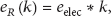
Figure 5 shows snapshots of the distribution of sensors of the nonuniform network shown in Figure 2 when running the Dynamic W-LEACH.

Figure 5

Sensor distribution for Dynamic W-LEACH on nonuniform WSN.

Figures 5(a) and 5(b) reflect the sensors distribution of the network at rounds 8440 and 8455, respectively. The figures clearly confirm that our algorithm can successfully handle nonuniform networks. At round 8440, which represents about 99.5% of the network lifetime, the network still functions with about 65% of its sensors, some of which represent the areas with less densities. This shows that our algorithm extends the lives of the sensors at low density areas so that it is ensured that data at these areas are not lost.

7.2. First Node Dies, Last Node Dies, and Average Sensor Lifetime

Figure 6 compares the averages of first node dies, last node dies, and average lifetime of sensors when LEACH and Dynamic W-LEACH are applied on the nonuniform network. Note that the figure also shows all the above listed metrics when Dynamic W-LEACH is applied on the evolving network.

Figure 6

First node dies, last node dies, and average lifetime for LEACH and Dynamic W-LEACH.

As it is clearly shown in the figure, Dynamic W-LEACH dramatically extends the first node dies, the last nodes dies, and the average lifetime when compared to LEACH. The most effected variable as it is shown the first node dies, which almost triples in its value. This shows that our algorithm tends to save the battery power in the different areas of the network as much as possible to make sure that the network captures all data equally. Even when the first sensor dies, the algorithm still tries to save the energy of network as much as possible and operates with less number of sensors that are scattered all over the area of nonuniform network. This can be concluded from the recorded results for last node dies and average lifetime of the networks, which are very close together.

The figure also shows that Dynamic W-LEACH performs in a similar way when applied to evolving networks as well. In fact, the evolving WSN that we use lives more than the nonuniform WSN as it can be seen from the last node dies values. Although the networks that we use for evolving and nonuniform networks have different settings, we present them in one figure to show that the algorithm performs similarly on both kinds of networks (nonuniform and evolving), since the nonuniform networks can be considered as snapshots of the evolving networks.

7.3. Number of Alive Sensors

Figure 7 shows the number of alive sensors with respect to rounds for LEACH and Dynamic W-LEACH for nonuniform and evolving networks.

Figure 7

Number of alive sensors versus rounds for LEACH and Dynamic W-LEACH.

As it is shown in the figure, the number of rounds of LEACH on nonuniform networks is around 5200 rounds with about the last 1000 rounds performing with less than 5 sensors. Whereas for Dynamic W-LEACH, the number of rounds is increased by more than 3000 rounds resulting in approximately 8500 rounds with about 90% of the sensors performing until the last 200 rounds where the number of alive sensors starts to drop. Similarly, Dynamic W-LEACH performs well for evolving networks. It saves the power of the sensors to later rounds. Even though the number of remaining alive sensors drops gradually at later rounds, the network lifetime is, however, increased.

7.4. Remaining Energy

Figure 8 presents the total remaining energy of nonuniform networks versus rounds for LEACH and Dynamic W-LEACH. It also presents the total remaining energy for Dynamic W-LEACH when applied to evolving networks.

Figure 8

Remaining energy versus rounds for LEACH and Dynamic W-LEACH.

The figure clearly shows that there is an extreme save of energy when Dynamic W-LEACH is applied to nonuniform as well as evolving networks. As it can be seen, these results support the above presented results of the number of alive sensors shown in Figure 7. Since Dynamic W-LEACH saves sensors’ lives to later rounds of the network, it operates with higher remaining energy than LEACH.

7.5. Data Accuracy

The data accuracy of Dynamic W-LEACH is evaluated using the ambient temperature values from the real dataset. As mentioned previously, the WSN contains 18 sensors. The accuracy of the data collected by the Dynamic W-LEACH is shown in Figure 9. The figure compares the average ambient temperature that is recorded by Dynamic W-LEACH to the actual average temperature. The average temperature values of Dynamic W-LEACH are calculated by finding the average value of the temperatures that are collected from the sensors, which are selected by the algorithm in every round to send data to their cluster head. The actual average temperature is basically the average value of all the temperatures that are recorded by all the sensors in the field. The figure shows that Dynamic W-LEACH maintains a high data accuracy. It records an average change of only 7 percent from the actual average.

Figure 9

Data accuracy of Dynamic W-LEACH.

7.6. Capturing Data in Areas with Events of Interests

We evaluate the performance of the Dynamic W-LEACH with adaptivity feature in capturing sudden bursts or events in the underlying values of the data. The performance is evaluated by introducing sudden events into the synthetic and real dataset files and then running the new data on Dynamic W-LEACH (original and modified version with adaptivity feature) to highlight the difference.

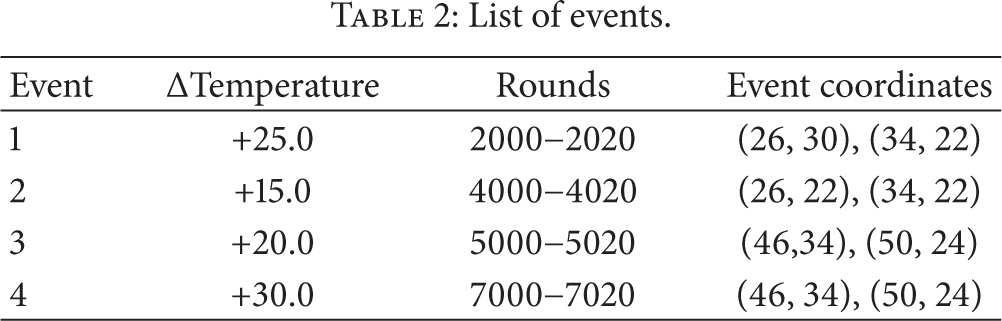
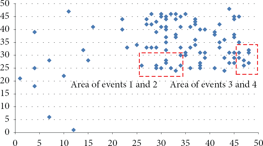
The sudden events that are used in the simulations are considered as sudden change in the ambient temperature that lasts for a specific period of time. In addition, the events take place over a specific area in the sensed field, meaning that only part of the sensors is able to detect the event. For the simulation, we define an event using three parameters: change in the underlying temperature, event duration in simulation rounds, and coordinates of the rectangular area in which the event lies. The events that we introduce in the synthetic dataset are shown in Table 2. Figure 14 shows the area of the events on the sensed field. From the figure, there are ten sensors in the event area for events 1 and 2, while for events 3 and 4 the number of sensors is 7.

Table 2

List of events.

Event	$\mathrm{\Delta }$ Temperature	Rounds	Event coordinates
1	+25.0	2000−2020	(26, 30), (34, 22)
2	+15.0	4000−4020	(26, 22), (34, 22)
3	+20.0	5000−5020	(46,34), (50, 24)
4	+30.0	7000−7020	(46, 34), (50, 24)

One factor that affects the performance of Dynamic W-LEACH in capturing sudden events is the number of sensors in the event area (event-area sensors) that eventually send the event-data to their cluster heads. Another factor is capturing the event throughout its whole duration. Clearly, the event is represented more accurately if a high number of event-area sensors send the event data and if the event data is recorded for the whole event. To evaluate the performance of Dynamic W-LEACH in capturing events of interest, we define a detection ratio metric as

$$\begin{array}{l}\text{Detection}\hspace{0.17em}\text{ratio}\\ \hspace{1em}=\frac{\text{actual}\hspace{0.17em}\hspace{0.17em}\text{number}\hspace{0.17em}\hspace{0.17em}\text{of}\hspace{0.17em}\hspace{0.17em}\text{events}-\text{sensors}\hspace{0.17em}\hspace{0.17em}\text{selected}}{\text{possible}\hspace{0.17em}\hspace{0.17em}\text{number}\hspace{0.17em}\hspace{0.17em}\text{of}\hspace{0.17em}\hspace{0.17em}\hspace{0.17em}\text{events}-\text{sensors}}.\end{array}$$

(8)

The possible number of event sensors is the maximum number of event sensors that can be selected in a given round. This value depends on the number of sensors that will send data to the cluster heads. Recall that Dynamic W-LEACH will set the number of sending sensors for each cluster in each round. To illustrate, consider the following case in which the current round has two clusters (A and B) and cluster B has three event sensors along with other sensors, while cluster A has no event sensors. Further, assume that each cluster will have one sensor sending data to the cluster head. In this case, the possible number of event sensors is one because at most one event sensor can be selected from cluster B. The actual number of event sensors selected can be either zero or one depending on whether or not any event sensor will eventually be chosen from cluster B. Note that possible number of event-sensors cannot be zero because in each round at least one sensor from each cluster will send data.

The detection ratio value becomes 1 if all the possible event sensors are actually selected by Dynamic W-LEACH to send the event data to their cluster heads.

Figures 10, 11, 12, and 13 show the detection ratio for the original and modified Dynamic W-LEACH algorithms under the events that are specified in Table 2. From the figures, we note that the detection ratio for the modified Dynamic W-LEACH is higher than that of the original Dynamic W-LEACH for the duration of the different events with the exception of few rounds. Outside the event window, the detection ratio value for the modified Dynamic W-LEACH becomes close to the original Dynamic W-LEACH. There are a few cases, rounds 2013 and 2017 in Figure 10 and round 4009 in Figure 11, in which the detection ratio of the modified W-LEACH is equal to or lower than that of the original W-LEACH. These 6 rounds might reflect some of the cases where far away sensors (sensors with low density that is less that $d_{\text{thresh}}$ ) are having low weights (lower than the sensors in the area of interest) and therefore attract the algorithm to choose them for sending data to their cluster heads. Again, we emphasize that a higher detection ratio during events means that the events are captured more accurately. Thus, it is clear that the modified Dynamic W-LEACH performs better than the original Dynamic W-LEACH in detecting sudden events by biasing its sensor selections towards the sensors in the events area.

Figure 10

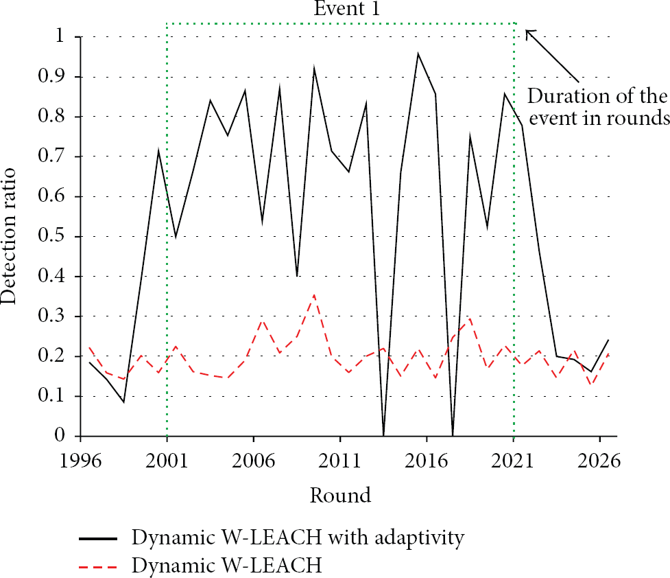
Sudden burst detection ratio of Dynamic W-LEACH for the synthetic dataset with event 1.

Figure 11

Sudden burst detection ratio of Dynamic W-LEACH for the synthetic dataset with event 2.

Figure 12

Sudden burst detection ratio of Dynamic W-LEACH for the synthetic dataset with event 3.

Figure 13

Sudden burst detection ratio of Dynamic W-LEACH for the synthetic dataset with event 4.

Figure 14

Position of the Events 1, 2, 3, and 4 on the sensed field.

We also simulate the modified Dynamic W-LEACH algorithm on the real dataset with a single event. Figure 15 shows the detection ratio for both versions of Dynamic W-LEACH during the event. It is obvious that in the case of the modified Dynamic W-LEACH the detection ratio is constantly one throughout the duration of the event resulting in a better event detection.

Figure 15

Sudden burst detection ratio of Dynamic W-LEACH for the real dataset (SensorScope deployment).

8. Related Work

8.1. LEACH-C and F-LEACH Algorithms

Both LEACH-C and F-LEACH algorithms are extensions from the same authors. We highlight them in this subsection. LEACH-C [3] assumes centralized CH election, where each sensor sends information about its location to the base station at the beginning of each round; then the base station uses an optimization algorithm, such as simulated annealing, to decide which sensors are to become CHs. The CHs are chosen based on their locations and their remaining energy such that clusters with more energy are candidates to be CHs. This gives a generally better distribution for CHs; however, it may reduce sensor lifetime due to the increase of communication between the sensors and the base station.

F-LEACH [6] assumes fixed clusters while only rotating the CHs for each cluster. This reduces the setup phase overhead that is performed in the beginning of each round since clusters are formed only once. It may, however, force a node to stay in a cluster with a CH that is further than a CH of a nearby cluster.

8.2. Other Extensions of LEACH Algorithm

Many algorithms extend LEACH in different ways. We highlight some major ones. We categorize the algorithms such that they are either based on the way of choosing the cluster heads [13–16, 22] or the way of routing the data to the sink of the network [14, 23–26].

Both M. C. M. Thein and T. Thein [13] and E-LEACH [14] are based on choosing CHs based on the remaining energy in sensors, such that in each round sensors with more remaining energy are good candidates to be chosen as CHs. V-LEACH [15] introduces the concept of vice-CH; a sensor that becomes CH if the current CH dies. This ensures that data is always delivered to the base station in the case where a CH dies in a specific round. Cooperative LEACH protocol [16] proposes the idea of using M cluster heads within a single cluster instead of using only one cluster head such that all chosen cluster heads cooperatively send data to the base station.

Multihop LEACH protocol [14] selects an optimal path between the cluster head and the base station such that less energy is consumed. FZ-LEACH [23, 25] proposes a solution for large clusters where routing to cluster heads consumes a great amount of energy. The solution concerns in defining where the far zones are and dividing the clusters into smaller ones where the data is then routed through multiple steps. A-LEACH [24] introduces the concept of helper nodes to help the cluster head for multihop routing. LEACH-MF [26] adopts the method of multilayer clustering to rout the sensed data.

8.3. Comparison with Selected Extensions of LEACH Algorithm

Unlike the above mentioned algorithms, our proposed algorithm, W-LEACH, is mainly based on extending LEACH in the way of data aggregation. It is, however, closer to the group of algorithms that extend LEACH in the way of selecting the cluster head, since the weights that W-LEACH introduces affect the CHs selection as well. We, therefore, state a comparison between our algorithm and this group of algorithms as they are close in the way of extending LEACH. See Table 3.

Table 3

Comparison between W-LEACH and other selected LEACH based algorithms.

Algorithm	Extension over LEACH
M. C. M. Thein and T. Thein [13]	$\mathrm{22}\mathrm{\%}$ longer network life
E-LEACH [14]	$\mathrm{30}\mathrm{\%}$ longer network life
V-LEACH [15]	$\mathrm{20}\mathrm{\%}$ better energy consumption
Cooperative LEACH [16]	$\mathrm{87}\mathrm{\%}$ longer network life
Our proposed W-LEACH	60% longer network life
	120% longer average node life
	195% more delay in first node dies

As it can be seen from Table 3, the two best algorithms in extending LEACH are Cooperative LEACH [16], which extends the network with approximate percentage of about 87%, and our algorithm W-LEACH, which extends the network life with approximate percentage of about 60%. Our algorithm, in addition, is tested on nonuniform and evolving networks. It also performs with 120% more in average node life than LEACH and 195% more in first node dies, which shows that the nodes are kept to later stages as it is shown from Figure 7.

9. Conclusion

This paper have proposed Dynamic W-LEACH; an adaptive data aggregation algorithm for WSNs that is based on LEACH-C algorithm [6]. Dynamic W-LEACH has added a number of extends to the original LEACH-C. The key feature that Dynamic W-LEACH is based on is the assumption that not all sensors readings are important every round since the readings might be so similar for nearby sensors. Not all sensors, hence, send data to their cluster heads every round. The total energy is, therefore, saved and the network lifetime is extended.

To achieve this key feature, W-LEACH deals with sensors weights; a new metric to decide which sensors should be assigned to be cluster heads and which should be assigned to be sending sensors. The weight metric is based on two main metrics, namely, the remaining energy of the sensor and the sensor density; a metric that shows how many sensors are in sensing range of this sensor. The number of sending sensors in each cluster for each round is decided based on the cluster density.

Another important feature is that Dynamic W-LEACH can handle sudden changes in the underlying data that can happen according to the occurrence of events in the sensed field. It highlights the area of interest so that the sensors in the event area are more likely chosen to send data to their cluster heads.

Simulation results show that W-LEACH extends the network life time and can work on both nonuniform and evolving WSNs while maintaining the accuracy of the data. Results also show that our algorithm is able to capture the events in the underlying data by recording the readings of the area of interest during the event.