Rossby Solitary Waves Generated by Wavy Bottom in Stratified Fluids

Abstract

Rossby solitary waves generated by a wavy bottom are studied in stratified fluids. From the quasigeostrophic vorticity equation including a wavy bottom and dissipation, by employing perturbation expansions and stretching transforms of time and space, a forced KdV-ILW-Burgers equation is derived through a new scale analysis, modelling the evolution of Rossby solitary waves. By analysis and calculation, based on the conservation relations of the KdV-ILW-Burgers equation, the conservation laws of Rossby solitary waves are obtained. Finally, the numerical solutions of the forced KdV-ILW-Burgers equation are given by using the pseudospectral method, and the evolutional feature of solitary waves generated by a wavy bottom is discussed. The results show that, besides the solitary waves, an additional harmonic wave appears in the wavy bottom forcing region, and they propagate independently and do not interfere with each other. Furthermore, the wavy bottom forcing can prevent wave breaking to some extent. Meanwhile, the effect of dissipation and detuning parameter on Rossby solitary waves is also studied. Research on the wavy bottom effect on the Rossby solitary waves dynamics is of interest in analytical geophysicalfluid dynamics.

1. Introduction

Rossby waves are a very important phenomenon in the oceanic and atmospheric motion. They determine the particular oceanographic weather, which is very important for shipping, fishing, hydroacoustics, and so on. Additionally, Rossby waves hold a vital role for the redistribution of energy throughout the world ocean. They attract lots of attention from oceanic and atmospheric scientists over the past years. Beginning with the pioneering research of Long [1] and Benney [2] on barotropic solitary waves, considerable works on solitary waves were carried out [3–11], and two theories were formed: KdV (Korteweg-de Vries) theory and BO (Benjamin-Ono) theory. The Rossby solitary waves described by the KdV equation are called classical solitary waves; the outstanding feature of this type of solitary waves is that they are very stable and also called soliton, while Rossby solitary waves described by the BO equation are called algebraic solitary waves and happen in deep fluids. The waveform of algebraic solitary waves vanishes algebraically as x → ∞. After the above two theories, Kubota et al. [12] presented a kind of new algebraic Rossby solitary waves which are described by the ILW (intermediate long waves) equation. Following the Kubota's work, Luo [13] also studied this kind of solitary waves and produced the ILW theory. In fact, the ILW equation can be reduced to the KdV equation and the BO equation in different depth fluids. Many mathematicians employed all kinds of methods to solve the above equations and obtained some inspiring results [14–17]. Everyone knows that the real oceanic and atmospheric motions can be modeled like a forced dissipative system. The effect of topography on the generation of Rossby solitary waves and the interaction of Rossby solitary waves with topography have been the subject of a lot of theoretical and experimental research. Most research has been confined to a fixed bottom, such as a concave or a convex bottom, a periodical bottom [18–22]. There is few research to consider the effect of a wavy bottom on Rossby solitary waves. In fact, we know that there are many factors to cause the ocean bottom wave, such as the vibrational wall in the experiment of the nonpropagating solitary wave [23], the shaking of the platform in ocean engineering and sediment transport [24–29], and the undulating substrate in the coating industry [30]. In addition, the longitudinal and transverse wave in an earthquake which happens occasionally in the ocean bottom can lead the ocean bottom to vary greatly. Moreover, waves are also an important outer factor to induce the ocean bottom to vary. In a word, the research on the effect of wavy bottom on Rossby solitary waves has a significant theoretical and application value. In the present work, we will present a new model (KdV-ILW-Burgers equation) to describe Rossby solitary waves excited by a wavy bottom. It is suitable for Rossby solitary waves in stratified fluids. By theoretical analysis and numerical simulation, the evolutional feature of Rossby solitary waves will be discussed, especially the wavy bottom effect and dissipation effect, and detuning parameter will be considered. The paper is organized as follows: in Section 2, a forced KdV-ILW-Burgers equation as governing model of Rossby solitary waves will be firstly derived by virtue of a new scale analysis from quasigeostrophic vorticity equation including wavy bottom and dissipation. It can be reduced to the KdV-Burgers equation and the KdV-BO-Burgers equation in different deep fluids, so we can conclude it is an extension of the former research. This is followed in Section 3 by the conservation relations of the KdV-ILW-Burgers equation and conservation laws of Rossby waves. Section 4 will be devoted to seek the numerical solutions of the forced KdV-ILW-Burgers equation and draw the waterfall plots. With the help of these waterfall plots, Rossby solitary waves excited by a wavy bottom and a nonwavy bottom will be compared. The effect of dissipation and detuning parameter on Rossby solitary waves will be studied. Finally, some conclusions will be given in Section 5.

2. Model and Governing Equation

The two-dimensional flow of an inviscid incompressible fluid will be considered. The coordinate system is sketched in Figure 1.

Figure 1:

The coordinate system.

From the basic equations (continuity equation, motion equation, and thermodynamics equation) of geophysical fluid dynamics, through the reasonable supposition, it is not difficult to obtain the nondimensional quasi-geostrophic potential vorticity equation as follows:

$\left(\frac{\partial }{\partial t}+\frac{\partial \mathrm{\Psi }}{\partial x}\frac{\partial }{\partial y}-\frac{\partial \mathrm{\Psi }}{\partial y}\frac{\partial }{\partial x}\right)\left[{\nabla }^{\mathrm{2}}\mathrm{\Psi }+\beta y+\frac{f^{\mathrm{2}}}{{\rho }_s}\frac{\partial }{\partial z}\left(\frac{{\rho }_s}{N^{\mathrm{2}}}\frac{\partial \mathrm{\Psi }}{\partial z}\right)\right]\hspace{0.17em}=\mathrm{0},$

(1)

see [31, 32] about the detailed derivation. Equation (1) is used to describe the inviscid, incompressible fluid motion, where Ψ is the dimensionless stream function; f is called Coriolis parameter; β is constant; N²(z) = – (g/ρ _s )(∂ ρ _s /∂ z) is the Brunt-Vaisala frequency, which is a measure of stability of the stratification; ρ _s means the density; ∇ ² = ∂ ²/∂ x² + ∂ ²/∂ y² denotes the two-dimensional Laplace operator.

We take total stream function Ψ as the distrubance stream ψ in a non-dimensional amplitude ∊ with superimposition of zonal flow. When ∊ ≪ 1, it is a weakly nonlinear problem, with which this paper deals. The total stream function thus becomes

$\mathrm{\Psi }=-{\int }^y\left(\stackrel{-}{u}\left(s,z\right)-c_{\mathrm{0}}+∊\alpha \right)ds+∊\psi ,$

(2)

the basic shear flows $\stackrel{-}{u}$ to be

$\stackrel{-}{u}\left(y,z\right)=\{\begin{array}{cc}u(y,z)\hfill & \mathrm{0}\le y\le L_{\mathrm{0}},\hfill \\ u_{\mathrm{0}}\hfill & L_{\mathrm{0}}<y\le L_{\mathrm{1}}.\hfill \end{array}$

(3)

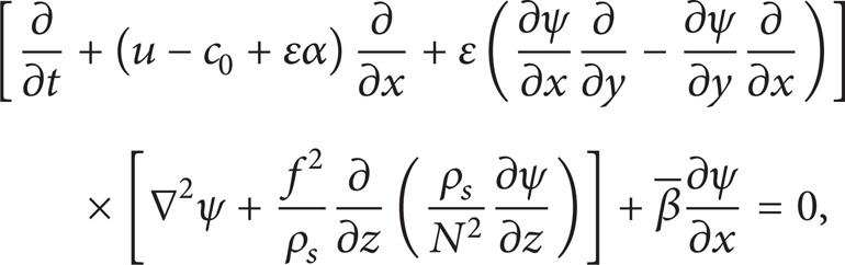
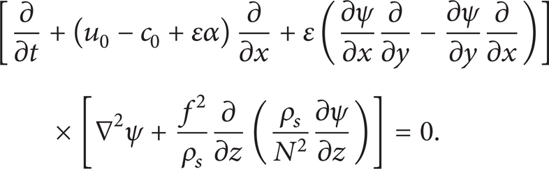
In (2) and (3), c₀ is a Rossby wave phase speed; ∊ is a small parameter, which stands for the ratio of vertical and horizontal length scale and is used to describe the degree of nonlinearity, strong or feeble; α is a detuning parameter and reflects the proximity of the system to a resonate state; y = 0, y = L₁ denote the southern and northern edges of the zonal flow in which latitudinal boundaries may exist. Substituting (2) and (3) into (1), in the domain [0, L₀], we have

$\left[\frac{\partial }{\partial t}+\left(u-c_{\mathrm{0}}+∊\alpha \right)\frac{\partial }{\partial x}+∊\left(\frac{\partial \psi }{\partial x}\frac{\partial }{\partial y}-\frac{\partial \psi }{\partial y}\frac{\partial }{\partial x}\right)\right]\hspace{0.17em}\times \left[{\nabla }^{\mathrm{2}}\psi +\frac{f^{\mathrm{2}}}{{\rho }_s}\frac{\partial }{\partial z}\left(\frac{{\rho }_s}{N^{\mathrm{2}}}\frac{\partial \psi }{\partial z}\right)\right]+\stackrel{—}{\beta }\frac{\partial \psi }{\partial x}=\mathrm{0},$

(4)

where $\stackrel{-}{\beta }=\beta -({\partial }^{\mathrm{2}}u/\partial y^{\mathrm{2}})-(f^{\mathrm{2}}/{\rho }_s)(\partial /\partial z)(({\rho }_s/N^{\mathrm{2}})(\partial u/\partial z))$ . While in the domain (L₀, L₁], the parameter β is smaller, here we take β = 0. Then the governing equation in this domain is

$\left[\frac{\partial }{\partial t}+\left(u_{\mathrm{0}}-c_{\mathrm{0}}+∊\alpha \right)\frac{\partial }{\partial x}+∊\left(\frac{\partial \psi }{\partial x}\frac{\partial }{\partial y}-\frac{\partial \psi }{\partial y}\frac{\partial }{\partial x}\right)\right]\hspace{0.17em}\times \left[{\nabla }^{\mathrm{2}}\psi +\frac{f^{\mathrm{2}}}{{\rho }_s}\frac{\partial }{\partial z}\left(\frac{{\rho }_s}{N^{\mathrm{2}}}\frac{\partial \psi }{\partial z}\right)\right]=\mathrm{0}.$

(5)

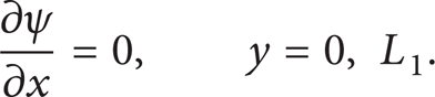
The side boundary conditions are defined as

$\frac{\partial \psi }{\partial x}=\mathrm{0},\hspace{1em}\hspace{1em}y=\mathrm{0},\hspace{0.17em}\hspace{0.17em}{L}_{\mathrm{1}}.$

(6)

In vertical direction, the upper boundary satisfies

${\rho }_s\psi \to \mathrm{0},\hspace{1em}\hspace{1em}z\to \infty .$

(7)

In lower boundary, considering the presence of topography and turbulent dissipation as well as heating, the governing equation from the thermal equation is

$\left(\frac{\partial }{\partial t}+\frac{\partial \mathrm{\Psi }}{\partial x}\frac{\partial }{\partial y}-\frac{\partial \mathrm{\Psi }}{\partial y}\frac{\partial }{\partial x}\right)\frac{\partial \mathrm{\Psi }}{\partial z}+\frac{N^{\mathrm{2}}}{f}\left[\frac{\partial h}{\partial t}+\frac{\partial \mathrm{\Psi }}{\partial x}\frac{\partial h}{\partial y}-\frac{\partial \mathrm{\Psi }}{\partial y}\frac{\partial h}{\partial x}\right]\hspace{0.17em}+{\lambda }_{\mathrm{0}}\frac{N^{\mathrm{2}}}{f}{\nabla }^{\mathrm{2}}\mathrm{\Psi }=Q,\hspace{1em}z=\mathrm{0}.$

(8)

here λ₀ ∇ ²Ψ denotes the vorticity dissipation effect caused by Ekman boundary layer, λ₀ is a dissipative coefficient and λ₀ ≥ 0, Q is the heating function and is used to eliminate the dissipation caused by shear flow, and h(x, y, t) is the topography function, especially the topography changes with time. In fact besides the previously mentioned factors causing the topography to change with time, the moving submarine and others can also be classified as a seabed topography related to time.

In (8), in order to achieve a balance among topography forcing, dissipation effect, and nonlinearity [33], we consider high order effect of topography forcing and dissipation as follows:

$h\left(x,y,t\right)={∊}^{\mathrm{2}}H\left(x,y,t\right),\hspace{1em}\hspace{1em}{\lambda }_{\mathrm{0}}={∊}^{\mathrm{3}/\mathrm{2}}\lambda .$

(9)

Here H(x, y, t) is high order topography function, and λ expresses high order dissipation coefficient. Because ∊ is a small parameter, (9) shows the weakly topography and dissipation effect. Then in order to eliminate the dissipation caused by shear flow $\stackrel{-}{u}$ , assume $Q=-{\lambda }_{\mathrm{0}}\mathrm{\hspace{0.17em}\hspace{0.17em}}(N^{\mathrm{2}}/f)(\partial \stackrel{-}{u}/\partial y)$ . By using (2) and (9), (8) can be rewritten as

$\frac{\partial }{\partial t}\left(\frac{\partial \psi }{\partial z}+∊\frac{N^{\mathrm{2}}}{f}H\right)+\left(\stackrel{—}{u}-c_{\mathrm{0}}+∊\alpha \right)\frac{\partial }{\partial x}\left(\frac{\partial \psi }{\partial z}+∊\frac{N^{\mathrm{2}}}{f}H\right)\hspace{0.17em}-\frac{\partial \stackrel{—}{u}}{\partial z}\frac{\partial \psi }{\partial x}+∊J\left[\psi ,\frac{\partial \psi }{\partial z}+∊\frac{N^{\mathrm{2}}}{f}H\right]+{∊}^{\mathrm{3}/\mathrm{2}}\lambda \frac{N^{\mathrm{2}}}{f}{\nabla }^{\mathrm{2}}\psi =\mathrm{0},$

(10)

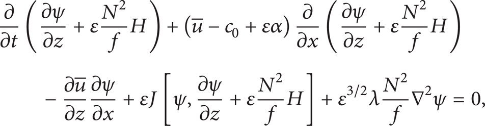
where J[A, B] = (∂ A/∂ x)(∂ B/∂ y) – (∂ A/∂ y)(∂ B/∂ x).

In order to achieve a balance between nonlinearity and dispersion, we introduce the following stretching transformation in the domain [0, L₀] [4, 6]:

$X={∊}^{\mathrm{1}/\mathrm{2}}x,\hspace{1em}\hspace{1em}T={∊}^{\mathrm{3}/\mathrm{2}}t,\hspace{1em}\hspace{1em}y=y,\hspace{1em}\hspace{1em}z=z.$

(11)

Expanding ψ as a power series in terms of ∊,

${\psi }_{[\mathrm{0},L_{\mathrm{0}}]}={\psi }_{\mathrm{1}}\left(X,y,z,T\right)+∊{\psi }_{\mathrm{2}}\left(X,y,z,T\right)+·.$

(12)

Substituting (11) into (4) and (10), we have

$\left[∊\frac{\partial }{\partial T}+\left(u-c_{\mathrm{0}}+∊\alpha \right)\frac{\partial }{\partial X}+∊\left(\frac{\partial \psi }{\partial X}\frac{\partial }{\partial y}-\frac{\partial \psi }{\partial y}\frac{\partial }{\partial X}\right)\right]\hspace{0.17em}\times \left[∊\frac{{\partial }^{\mathrm{2}}\psi }{\partial X^{\mathrm{2}}}+\frac{{\partial }^{\mathrm{2}}\psi }{\partial y^{\mathrm{2}}}+\frac{f^{\mathrm{2}}}{{\rho }_s}\frac{\partial }{\partial z}\left(\frac{{\rho }_s}{N^{\mathrm{2}}}\frac{\partial \psi }{\partial z}\right)\right]+\stackrel{—}{\beta }\frac{\partial \psi }{\partial X}=\mathrm{0},$

(13)

$∊\frac{\partial }{\partial T}\left(\frac{\partial \psi }{\partial z}+∊\frac{N^{\mathrm{2}}}{f}H\right)+\left(\stackrel{—}{u}-c_{\mathrm{0}}+∊\alpha \right)\frac{\partial }{\partial X}\hspace{0.17em}\times \left(\frac{\partial \psi }{\partial z}+∊\frac{N^{\mathrm{2}}}{f}H\right)-\frac{\partial \stackrel{—}{u}}{\partial z}\frac{\partial \psi }{\partial X}+∊J^{\prime }\left[\psi ,\frac{\partial \psi }{\partial z}+∊\frac{N^{\mathrm{2}}}{f}H\right]\hspace{0.17em}+∊\lambda \frac{N^{\mathrm{2}}}{f}\left(∊\frac{{\partial }^{\mathrm{2}}\psi }{\partial X^{\mathrm{2}}}+\frac{{\partial }^{\mathrm{2}}\psi }{\partial y^{\mathrm{2}}}\right)=\mathrm{0},\hspace{1em}z=\mathrm{0},$

(14)

where J′[A, B] = (∂ A/∂ X)(∂ B/∂ y) – (∂ A/∂ y)(∂ B/∂ X).

It is convenient to introduce two linear differential operators defined as

$\begin{array}{c}M=\left(u-c_{\mathrm{0}}\right)\left(\frac{{\partial }^{\mathrm{2}}}{\partial y^{\mathrm{2}}}+\frac{f}{{\rho }_s}\frac{\partial }{\partial z}\left(\frac{{\rho }_s}{s}\frac{\partial }{\partial z}\right)+\frac{\stackrel{—}{\beta }}{u-c_{\mathrm{0}}}\right),\\ L=\left(u-c_{\mathrm{0}}\right)\frac{\partial }{\partial z}-\frac{\partial \stackrel{-}{u}}{\partial z}.\end{array}$

(15)

Assuming that ψ₁ has the form of ψ₁ = A(X, T)ϕ₁(y, z), here A(X, T) is regarded as the amplitude of Rossby solitary waves. Then substituting (12) into (13) and boundary conditions (6), (7), and (14) can lead to the following perturbation equation and boundary conditions of O(∊⁰):

$\begin{array}{c}M\left({\varphi }_{\mathrm{1}}\right)=\mathrm{0},\\ L\left({\varphi }_{\mathrm{1}}\right)=\mathrm{0},\hspace{1em}\hspace{1em}z=\mathrm{0},\\ {\rho }_s{\varphi }_{\mathrm{1}}\to \mathrm{0},\hspace{1em}\hspace{1em}z\to \infty ,\\ {\varphi }_{\mathrm{1}}=\mathrm{0},\hspace{1em}\hspace{1em}y=\mathrm{0}.\end{array}$

(16)

Equation (16) is an eigenvalue problem, describing the space structure of the wave along direction; the boundary value at y = L₀ can be obtained from (5). Once u(y, z) is specified, ϕ₁(y, z) can be determined. In other words, the space structure of the wave along y, z direction can be described once u(y, z) is given, while the amplitude A(X, T) cannot be got in the order O(∊⁰).

In order to derive the evolution of the amplitude A(X, T), let us proceed to higher order equation. For O(∊¹), we can obtain the following perturbation equation and boundary conditions:

$\begin{array}{c}M\left(\frac{\partial {\psi }_2}{\partial X}\right)=\left(\frac{\partial A}{\partial T}+\alpha \frac{\partial A}{\partial X}\right)\frac{\stackrel{—}{\beta }}{u-c_0}{\varphi }_1+A\frac{\partial A}{\partial X}\left[{\varphi }_1\frac{\partial }{\partial y}\left(\frac{\stackrel{—}{\beta }}{u-c_0}{\varphi }_1\right)-\frac{\partial {\varphi }_1}{\partial y}\left(\frac{\stackrel{—}{\beta }}{u-c_0}{\varphi }_1\right)\right]-\left(u-c_0\right){\varphi }_1\frac{{\partial }^{3}A}{\partial X^3},\\ L\left(\frac{\partial {\psi }_{\mathrm{2}}}{\partial X}\right)=-\left(\frac{\partial A}{\partial T}+\alpha \frac{\partial A}{\partial X}\right)\frac{\partial {\varphi }_{\mathrm{1}}}{\partial z}-A\frac{\partial A}{\partial X}\times \left({\varphi }_{\mathrm{1}}\frac{{\partial }^{\mathrm{2}}{\varphi }_{\mathrm{1}}}{\partial y\partial z}-\frac{\partial {\varphi }_{\mathrm{1}}}{\partial y}\frac{\partial {\varphi }_{\mathrm{1}}}{\partial z}\right)-\frac{N^{\mathrm{2}}}{f}\lambda A\frac{{\partial }^{\mathrm{2}}{\varphi }_{\mathrm{1}}}{\partial y^{\mathrm{2}}}-\frac{N^{\mathrm{2}}}{f}\left(u-c_{\mathrm{0}}\right)\frac{\partial H}{\partial X},\hspace{1em}z=\mathrm{0},\\ {\rho }_s{\psi }_{\mathrm{2}}\to \mathrm{0},\hspace{1em}\hspace{1em}z\to \infty ,\\ \frac{\partial {\psi }_{\mathrm{2}}}{\partial X}=\mathrm{0},\hspace{1em}\hspace{1em}y=\mathrm{0}.\end{array}$

(17)

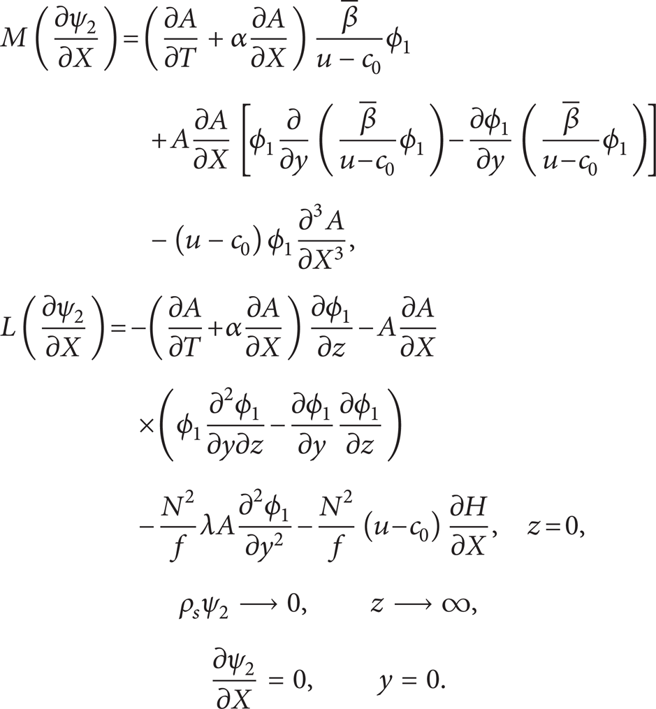
Multiplying both sides of the first equation of (17) by (ρ _s ϕ₁)/(u – c₀) and integrating it over [0, L₀] about y and [0, ∞] about z can lead to

$\begin{array}{c}\frac{\partial }{\partial X}[{\int }_{\mathrm{0}}^{+\infty }{{\rho }_s\left({\varphi }_{\mathrm{1}}\frac{\partial }{\partial y}{\psi }_{\mathrm{2}}-{\psi }_{\mathrm{2}}\frac{\partial }{\partial y}{\varphi }_{\mathrm{1}}\right)|}_{y=\mathrm{0}}^{y=L_{\mathrm{0}}}dz\hspace{0.17em}+{\int }_{\mathrm{0}}^{L_{\mathrm{0}}}{\frac{f^{\mathrm{2}}{\rho }_s}{N^{\mathrm{2}}}\left({\varphi }_{\mathrm{1}}\frac{\partial }{\partial z}{\psi }_{\mathrm{2}}-{\psi }_{\mathrm{2}}\frac{\partial }{\partial z}{\varphi }_{\mathrm{1}}\right)|}_{z=\mathrm{0}}^{\text{z}=\infty }dy]\\ \hspace{1em}={\int }_{\mathrm{0}}^{L_{\mathrm{0}}}{\int }_{\mathrm{0}}^{+\infty }\left(\frac{\partial A}{\partial T}+\alpha \frac{\partial A}{\partial X}\right)\frac{{\rho }_s{\varphi }_{\mathrm{1}}^{\mathrm{2}}\stackrel{—}{\beta }}{{\left(u-c_{\mathrm{0}}\right)}^{\mathrm{2}}}-\frac{{\partial }^{\mathrm{3}}A}{\partial X^{\mathrm{3}}}{\rho }_s{\varphi }_{\mathrm{1}}^{\mathrm{2}}+A\frac{\partial A}{\partial X}\times \left[\frac{{\rho }_s{\varphi }_{\mathrm{1}}^{\mathrm{2}}}{u-c_{\mathrm{0}}}\frac{\partial }{\partial y}\left(\frac{{\varphi }_{\mathrm{1}}\stackrel{—}{\beta }}{u-c_{\mathrm{0}}}\right)-\frac{{\rho }_{\text{s}}{\varphi }_{\mathrm{1}}^{\mathrm{2}}\stackrel{—}{\beta }}{{\left(u-c_{\mathrm{0}}\right)}^{\mathrm{2}}}\frac{\partial {\varphi }_{\mathrm{1}}}{\partial y}\right]dz\hspace{0.17em}dy.\end{array}$

(18)

In (18), ϕ₁, ψ₂ have been given at z = 0, z → ∞, and y = 0, but is absent at y = L₀. Next, we will solve the problem.

For (5) in the domain (L₀, L₁], we adopt thefollowing Gardner-Morikawa transformations [4, 6]:

$\xi =x,\hspace{1em}\hspace{1em}T={∊}^{\mathrm{3}/\mathrm{2}}t,\hspace{1em}\hspace{1em}y=y,\hspace{1em}\hspace{1em}\eta ={∊}^{\mathrm{1}/\mathrm{2}}z,$

(19)

here T and η are slow variables. The disturbance streamfunction ψ is set $\psi =\stackrel{—}{\psi }(\xi ,y,\eta ,T)$ . Then introducing (19) into (5), we obtain the lowest-order equation for the domain (L₀, L₁]:

$\left(u_{\mathrm{0}}-c_{\mathrm{0}}\right)\frac{\partial }{\partial \xi }\left(\frac{{\partial }^{\mathrm{2}}}{\partial {\xi }^{\mathrm{2}}}+\frac{{\partial }^{\mathrm{2}}}{\partial y^{\mathrm{2}}}\right)\stackrel{—}{\psi }=\mathrm{0}.$

(20)

When the integration constant is taken as zero, it is easy to obtain

$\left(\frac{{\partial }^{\mathrm{2}}}{\partial {\xi }^{\mathrm{2}}}+\frac{{\partial }^{\mathrm{2}}}{\partial y^{\mathrm{2}}}\right)\stackrel{—}{\psi }=\mathrm{0}.$

(21)

By virtue of the boundary condition ${\partial \stackrel{-}{\psi }/\partial \xi |}_{y=L_{\mathrm{1}}}=\mathrm{0}$ , we get the solution of (19) as follows:

$\stackrel{—}{\psi }\left(\xi ,y,\eta ,T\right)\hspace{1em}=\frac{\mathrm{1}}{\mathrm{2}\pi }{\int }_{-\infty }^{+\infty }F\left({\stackrel{—}{\psi }|}_{y=L_0}\right)\frac{\sinh p\left(L_{\mathrm{1}}-y\right)}{\sinh p\left(L_{\mathrm{1}}-L_{\mathrm{0}}\right)}{e}^{ip\xi }dp,$

(22)

where $F({\stackrel{—}{\psi }|}_{y=L_0})$ expresses the Fourier transformation of ${\stackrel{—}{\psi }|}_{y=L_{\mathrm{0}}}$ . Differentiating (22) with respect to y, we have

$\frac{\partial \stackrel{—}{\psi }\left(\xi ,y,\eta ,T\right)}{\partial y}=\frac{-\mathrm{1}}{\mathrm{2}\pi }{\int }_{-\infty }^{+\infty }F\left({\stackrel{—}{\psi }|}_{y=L_0}\right)p\frac{\cosh p\left(L_{\mathrm{1}}-y\right)}{\sinh p\left(L_{\mathrm{1}}-L_{\mathrm{0}}\right)}{e}^{ip\xi }dp.$

(23)

Assuming the solution matches smoothly at y = L₀, then we have

$\begin{array}{c}{\psi }_{\mathrm{1}}\left(X,L_{\mathrm{0}},z,T\right)+∊{\psi }_{\mathrm{2}}\left(X,L_{\mathrm{0}},z,T\right)=\stackrel{—}{\psi }\left(\xi ,L_{\mathrm{0}},\eta ,T\right)+O\left({∊}^{\mathrm{2}}\right),\\ {\frac{\partial {\psi }_{\mathrm{1}}\left(X,y,z,T\right)}{\partial y}|}_{y=L_{\mathrm{0}}}{+∊\frac{\partial {\psi }_{\mathrm{2}}\left(X,y,z,T\right)}{\partial y}|}_{y=L_{\mathrm{0}}}\hspace{0.17em}{=\frac{\partial \stackrel{—}{\psi }\left(\xi ,y,\eta ,T\right)}{\partial y}|}_{y=L_{\mathrm{0}}}+O\left({∊}^{\mathrm{2}}\right).\end{array}$

(24)

From (24), we get

$A\left(X,T\right){\varphi }_{\mathrm{1}}\left(L_{\mathrm{0}},z\right)=\stackrel{—}{\psi }\left(\xi ,L_{\mathrm{0}},\eta ,T\right),\hspace{1em}\hspace{1em}{\psi }_{\mathrm{2}}\left(X,L_{\mathrm{0}},z,T\right)=\mathrm{0}.$

(25)

Based on (23) and (25), we obtain

$\frac{\partial \stackrel{—}{\psi }\left(\xi ,L_{\mathrm{0}},\eta ,T\right)}{\partial y}=\frac{-∊}{P}\frac{\partial }{\partial X}{\int }_{-\infty }^{+\infty }A\left(X^{\prime },T\right){\varphi }_{\mathrm{1}}\left(L_{\mathrm{0}},z\right)\coth \frac{\pi }{P}\left(X-X^{\prime }\right)d{X}^{\prime },$

(26)

where P = 2 (L₁ – L₀)∊, and L₁ – L₀ is taken as big enough to satisfy P ≥ O(1). There is no need to require L₁ → ∞. It is easy to find that ${\partial \stackrel{-}{\psi }/\partial y|}_{(y=L_{\mathrm{0}})}=O(∊)$ . From (24) and (26), we have

$\begin{array}{c}{\left(\frac{\partial {\stackrel{-}{\varphi }}_{\mathrm{1}}}{\partial y}\right)|}_{(y=L_{\mathrm{0}})}=\mathrm{0},\\ \frac{\partial {\psi }_{\mathrm{2}}\left(X,L_{\mathrm{0}},z,T\right)}{\partial y}=\frac{-\mathrm{1}}{P}\frac{\partial }{\partial X}{\int }_{-\infty }^{+\infty }A\left(X^{\prime },T\right){\varphi }_{\mathrm{1}}\left(L_{\mathrm{0}},z\right)\coth \frac{\pi }{P}\left(X-X^{\prime }\right)d{X}^{\prime }.\end{array}$

(27)

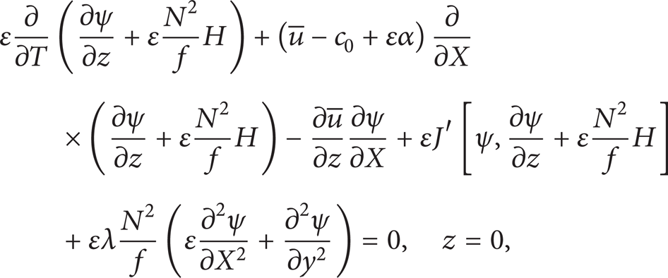
Substituting the boundary conditions in (16), (17), (25), and (27) into (18), after tedious calculation, we can obtain the following governing equation of the amplitude of Rossby solitary waves (see Appendix A about the detailed calculation):

$\frac{\partial A}{\partial T}+\alpha \frac{\partial A}{\partial X}+a_{\mathrm{1}}A\frac{\partial A}{\partial X}+a_{\mathrm{2}}\frac{{\partial }^{\mathrm{3}}A}{\partial X^{\mathrm{3}}}+a_{\mathrm{3}}\lambda A+a_{\mathrm{4}}\frac{{\partial }^{\mathrm{2}}}{\partial X^{\mathrm{2}}}{\int }_{-\infty }^{+\infty }A\left(X^{\prime },T\right)\coth \frac{\pi }{P}\left(X-X^{\prime }\right)d{X}^{\prime }=a_{\mathrm{5}}\frac{\partial H}{\partial X}.$

(28)

Equation (28) is a forced integrodifferential equation including dissipation effect and topography effect. The term a₃λA means dissipation effect and has the same physical meaning with the term A _XX in Burgers equation; the term a₅ (∂ H/∂ X) means topographic forcing. It is easy to find that (28) is a composite equation, and from it we can obtain other equations. When a₃ = a₄ = a₅ = 0, it becomes the KdV equation; when a₄ = a₅ = 0, we call it KdV-Burgers equation; when a₂ = a₃ = a₅ = 0, it becomes the so-called ILW (Intermediately Long Wave) equation. So here we call (28) forced KdV-ILW-Burgers equation. This is a new equation and firstly obtained here.

It should be noted that in the case of L₁ → ∞, then coth(X – X′)/P → 1/(X – X′), and (28) reduces to the so-called KdV-BO-Burgers equation; in the opposite limit, (28) reduces to the KdV-Burgers equation, so we can conclude that it is an extension of the KdV-Burgers equation [34] and the BO-Burgers equation [35].

3. Conservation Laws

Conservation laws are an important research subject in geophysical fluid dynamics, for they generate strong insights into how flows are dynamically constrained. Such laws have important application to the fluid system as a whole or to wavelike excitations of the fluid. The purpose of the section is to discuss the effect of dissipation and topography on the conservation laws of Rossby solitary waves.

Here we assume that A, A _X , A _XX , A _XXX vanish as X → ∞ and for convenience to define operator $S(A)={\int }_{-\infty }^{+\infty }A(X^{\prime },T)\coth (\pi /P)(X-X^{\prime })d{X}^{\prime }$ . First let us integrate (28) itself with respect to X from – ∞ to + ∞, then it follows

$\frac{d}{dT}{\int }_{-\infty }^{\infty }A\hspace{0.17em}dX+a_{\mathrm{3}}\lambda {\int }_{-\infty }^{\infty }A\hspace{0.17em}dX=a_{\mathrm{5}}{\int }_{-\infty }^{\infty }\frac{\partial H}{\partial X}dX.$

(29)

It shows that in the absence of dissipation (λ = 0), for a localized topographic forcing (H = 0 as |X| → ∞), the mass of the solitary waves is conserved; for a infinite topographic forcing (H ≠ 0 as |X| → ∞), the mass conservation is destroyed. In the presence of dissipation, topography effect is neglected, and the following relation exists:

${\int }_{-\infty }^{\infty }A\hspace{0.17em}dX=e^{-a_{\mathrm{3}}\lambda T}{\int }_{-\infty }^{\infty }A\left(X,\mathrm{0}\right)dX.$

(30)

It indicates that the mass of solitary waves decreases exponentially with the time evolution and the increasing of dissipation coefficient λ.

Next, when (28) is multiplied by A and integrated with respect to X between – ∞ and + ∞ and by employing the property of $S:{\int }_{-\infty }^{+\infty }f(X)S(g(X))dX=-{\int }_{-\infty }^{+\infty }g(X)S(f(X))dX$ , in which f, g are arbitrary functions vanishing at infinity, we get

$\frac{d}{dT}{\int }_{-\infty }^{\infty }{A}^{\mathrm{2}}dX+\mathrm{2}{a}_{\mathrm{3}}\lambda {\int }_{-\infty }^{\infty }{A}^{\mathrm{2}}dX=\mathrm{2}{a}_{\mathrm{5}}{\int }_{-\infty }^{\infty }A\frac{\partial H}{\partial X}dX.$

(31)

It indicates that the changing of the momentum of solitary waves is due to the presence of dissipation effect and topographic forcing. The momentum of solitary waves is conserved without dissipation effect and topographic forcing. Especially, in the presence of dissipation while the topographic forcing is absent, we obtain

${\int }_{-\infty }^{+\infty }{A}^{\mathrm{2}}dX=\exp \left(-\mathrm{2}{a}_{\mathrm{3}}\lambda T\right){\int }_{-\infty }^{+\infty }{A}^{\mathrm{2}}\left(X,\mathrm{0}\right)dX.$

(32)

It follows that the momentum of solitary waves decreases exponentially with the time evolution and the increasing of dissipation coefficient λ. Furthermore, its rate of decay is bigger than the mass of solitary waves.

Following, multiplying (28) by (A² – a₄S(A _X )/a₁) and meanwhile differentiating (28) with respect to X and multiplying it by (−2a₂A _X /a₁ + a₄S(A)/a₁), and then the above two equations are added together, integrated with respect to X between – ∞ and + ∞, after tedious calculation, we will obtain that

$\begin{array}{c}\frac{d}{dT}{\int }_{-\infty }^{+\infty }\left[\frac{A^{\mathrm{3}}}{\mathrm{3}}-\frac{a_{\mathrm{2}}}{a_{\mathrm{1}}}{A_X}^2+\frac{a_{\mathrm{4}}}{a_{\mathrm{1}}}{A}_{X}S\left(A\right)\right]dX\hspace{0.17em}+a_{\mathrm{3}}\lambda {\int }_{-\infty }^{+\infty }\left[A^{\mathrm{3}}-\frac{\mathrm{2}{a}_{\mathrm{2}}}{a_{\mathrm{1}}}{A_X}^2+\frac{\mathrm{2}{a}_{\mathrm{4}}}{a_{\mathrm{1}}}{A}_{X}S\left(A\right)\right]dX\\ =a_{\mathrm{5}}{\int }_{-\infty }^{\infty }[A^{\mathrm{2}}\frac{\partial H}{\partial X}-\frac{\mathrm{2}{a}_{\mathrm{2}}}{a_{\mathrm{1}}}{A}^{\mathrm{2}}\frac{{\partial }^{\mathrm{2}}H}{\partial X^{\mathrm{2}}}+\frac{a_{\mathrm{4}}}{a_{\mathrm{1}}}S\left(A\right)\frac{{\partial }^{\mathrm{2}}H}{\partial X^{\mathrm{2}}}-\frac{a_{\mathrm{4}}}{a_{\mathrm{1}}}S\left(A_X\right)\frac{\partial H}{\partial X}]dX.\end{array}$

(33)

Using a customary designation we can refer to ${\int }_{-\infty }^{+\infty }\hspace{0.17em}[A^{\mathrm{3}}/\mathrm{3}-(a_{\mathrm{2}}/a_{\mathrm{1}}){A_X}^2+(a_{\mathrm{4}}/a_{\mathrm{1}})A_{X}S(A)]dX$ as energy of solitary waves, although it is not necessarily identifiable with energy in the original physical problem. It shows that the energy of solitary waves is conserved if the dissipation effect and topographic forcing are not considered; that is, the changing of the energy of solitary waves is also due to the presence of dissipation effect and topographic forcing.

Further, let us consider the following quantity:

$C_{\mathrm{1}}=\frac{{\int }_{-\infty }^{\infty }{XA}_{T}dX}{{\int }_{-\infty }^{\infty }A\hspace{0.17em}dX},$

(34)

which is regarded as velocity of the center of gravity for ensemble of such waves in [36]. By calculation, we can deduce that when dissipation effect is absent, the topographic forcing do not exist or the topographic forcing is local, and the topography do not change with time, the velocity of the center of gravity for ensemble of solitary waves is conserved; the conservation is destroyed when these conditions cannot be satisfied (see Appendix B).

To make further progress, we proceed to construct the following quantity:

$C_{\mathrm{2}}={\int }_{-\infty }^{+\infty }\frac{A^{\mathrm{4}}}{\mathrm{4}}-\frac{\mathrm{3}{a}_{\mathrm{2}}A{A_X}^{\mathrm{2}}}{a_{\mathrm{1}}}+\frac{\mathrm{9}{a}_{\mathrm{2}}{A_{XX}}^{\mathrm{2}}}{{a_1}^2}+\frac{a_{\mathrm{4}}{A}^{\mathrm{2}}S\left(A\right)}{\mathrm{4}{a}_{\mathrm{1}}}dX.$

(35)

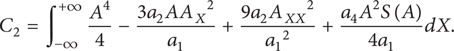
By calculation we can verify that C₂ is also a time-invariant quantity without dissipation and topographic forcing.

Heretofore, five conservation quantities of (28) have been obtained, then we will wonder that weather the KdV-ILW-Burgers equation has an infinity of conservation quantities similar to the KdV equation in the absence of dissipation and topographic forcing. Besides the conservation quantities, the analytical solution and the related property of (28) with H = 0 are also worth studying. It has an important value for understanding and realizing the feature of solitary waves. These problems are open, and we will not discuss them here owing to space reasons.

4. Numerical Solutions and Discussion

In this section, we will study the evolutional feature of Rossby solitary waves under the influence of a wavy bottom; especially we will focus on the difference of solitary waves which are excited by a wavy bottom and a non-wavy bottom and the effect of dissipation and detuning parameter. While, as we know, the forced KdV-ILW-Burgers equation has no analytical solution, we have to seek its numerical solutions by the pseudospectral method [37]. In (28), once the shear flows $\stackrel{-}{u}$ and topography function H as well as dissipation coefficient λ are given, with the help of (16), it is easy to obtain the coefficients in (28). To simplify the calculation, to pay attention to the evolutional feature of Rossby solitary waves under the influence of a wavy bottom and dissipation, and to state the difference of solitary waves which is excited by different bottoms, without loss of generality, we take a₁ = – 0.5, a₂ = 0.5, a₃ = 1, a₄ = – 0.5, and a₅ = 1 and put the initial value A = 0 at T = 0. In the present calculations, the bottom function H is supposed to be H(X, T) = hsin(kX + ωT), where h is the constant amplitude of the vary bottom, k is the wave number of the harmonic vibration, and ω is the frequency of the harmonic vibration. And let h = 0.5, k = 0.05π.

4.1. Comparison between Wavy Bottom and Nonwavy Bottom

The simulating results for the wavy bottom wave and the non-wavy bottom wave in different time scale are shown in Figures 2, 3, 4, and 5, where the detuning parameter is taken as zero; that is, the resonant state and the dissipation effect are neglected. By comparing Figure 1 to Figure 2, it is easy to find that there are both solitary waves generated in the bottom forcing region and their shapesare alike the bottom topography. Besides the soliatry waves alike the bottom topography, there are also a harmonic wave in the wavy topography forcing region, while the harmonic wave does not exist in the non-wavy topography forcing region. Furthermore, the solitary waves do not interfere with the harmonic wave in wavy topographic forcing region and propagate independently. With the evolution of time, the phenomenon gets more obvious. When the time scale is 40, from Figure 4, we can find that there are dramatic variations even fragmentation on the solitary waves in the forcing region for non-wavy bottom. This phenomenon occurs because the nonlinearity is disequilibrium with the dispersion. While from Figure 5, for the waves generated by wavy topography, there are still solitary waves together with an additional harmonic wave in the forcing region, the wave-breaking phenomenon does not occur, the wave form remains invariable, and just the amplitude decreases gradually with time evolution. We can conclude that wavy bottom forcing can prevent wave breaking to some extent.

Figure 2:

Solitary waves excited by nonwavy topography in the absence of dissipation (λ = 0, ω = 0, α = 0, T ∊ [0,20]).

Figure 3:

Solitary waves excited by wavy topography in the absence of dissipation $(\lambda =\mathrm{0},\hspace{0.17em}\omega =\mathrm{0.1},\hspace{0.17em}\alpha =\mathrm{0},\hspace{0.17em}T∊[\mathrm{0,20}])$ .

Figure 4:

Solitary waves excited by nonwavy topography in the absence of dissipation $(\lambda =\mathrm{0},\hspace{0.17em}\omega =\mathrm{0},\hspace{0.17em}\alpha =\mathrm{0},\hspace{0.17em}T∊[\mathrm{0,40}])$ .

Figure 5:

Solitary waves excited by wavy topography in the absence of dissipation $(\lambda =\mathrm{0},\hspace{0.17em}\omega =\mathrm{0.1},\hspace{0.17em}\alpha =\mathrm{0},\hspace{0.17em}T∊[\mathrm{0,40}])$ .

4.2. Effect of Dissipation and Detuning Parameter

Figure 6 shows the solitary waves excited by a nonwavy bottom with the dissipative coefficient λ = 0.05 and the detuning parameter α = 0. It is used to explain the influence of dissipation on solitary waves generated by topography. Comparing Figure 6 to Figure 2, it is not difficult to find that dissipation effect causes the amplitude of solitary waves in the forcing region to decrease.

Figure 6:

Solitary waves excited by nonwavy topography in the presence of dissipation $(\lambda =\mathrm{0.05},\hspace{0.17em}\omega =\mathrm{0},\hspace{0.17em}\alpha =\mathrm{0},\hspace{0.17em}T∊[\mathrm{0,20}])$ .

Figures 7 and 8 are used to show the effect of detuning parameter on solitary waves generated by a non-wavy bottom. In Figures 7 and 8, the detuning parameter α is taken −1 and 2, respectively. By comparing Figure 4 to Figures 7 and 8, the following conclusions can be obtained.

1. The amplitudes of solitary waves in the forcing region decrease with increasing of the detuning parameter |α|. When α = 0, which corresponds to the resonant state (Figure 4), the amplitudes of waves increase extremely rapidly. The wave-breaking phenomenon is easy to happen. With the increasing of detuning parameter |α|, the amplitudes of waves decrease, and the waves have more difficulties to break.

2. As α = 0, solitary waves are excited in the forcing region, remain steady, and do not propagate; as α < 0, solitary waves are excited in the forcing region and propagate toward the upstream, while as α > 0, the solitary waves are excited in the forcing region and propagate toward the downstream.

Figure 7:

Solitary waves excited by nonwavy topography in the absence of dissipation $(\lambda =\mathrm{0},\hspace{0.17em}\omega =\mathrm{0},\hspace{0.17em}\alpha =-\mathrm{1},\hspace{0.17em}T∊[\mathrm{0,40}])$ .

Figure 8:

Solitary waves excited by nonwavy topography in the absence of dissipation $(\lambda =\mathrm{0},\hspace{0.17em}\omega =\mathrm{0},\hspace{0.17em}\alpha =\mathrm{2},\hspace{0.17em}T∊[\mathrm{0,40}])$ .

5. Conclusions

In the paper, we derive a forced KdV-ILW-Burgers equation including dissipation term, wavy bottom forcing from the quasigeostrophic vorticity equation through a new scale analysis that is presented in the paper, analyze the conservation relations of the KdV-ILW-Burgers equation, and obtain the conservation laws of Rossby solitary waves; that is, mass, momentum, energy, and velocity of the center of gravity of Rossby solitary waves are conserved without dissipation. Detailed numerical results are presented by employing the pseudo-spectral method, compare Rossby solitary waves excited by a wavy bottom to a nonwavy bottom, and demonstrate the effect of dissipation and detuning parameter. The results show that besides the solitary waves, an additional harmonic wave appears in the wavy bottom forcing region, and they propagate independently and do not interfere with each other. Furthermore, wavy bottom forcing can prevent wave breaking to some extent. This is a useful supplement of the classical geophysical theory of fluid dynamics. Meanwhile, we can conclude that the amplitudes of solitary waves in the forcing region decrease with increasing of dissipative coefficient λ and |α|. When |α| is bigger, the waves are more difficult to break.

Several open problems are presented in this paper

1. If the KdV-ILW-Burgers equation has an infinity of conservation quantities in the absence of dissipation?

2. The analytical solution and the related property of the KdV-ILW-Burgers equation are also worth of studying.

They have an important value for understanding and realizing the feature of solitary waves.