Dynamic Modeling and Fu zzy Self-Tuning Disturbance Decoupling Control for a 3-DOF Serial-Parallel Hybrid Humanoid Arm

Abstract

A unique fuzzy self-tuning disturbance decoupling controller (FSDDC) is designed for a serial-parallel hybrid humanoid arm (HHA) to implement the throwing trajectory-tracking mission. Firstly, the dynamic model of the HHA is established and the input signal of the throwing process is obtained by studying the throwing process of human's arm. Secondly, the FSDDC, incorporating the disturbance decoupling controller (DDC) and the fuzzy logic controller (FLC), is designed to ensure trajectory tracking of the HHA in the presence of uncertainties and disturbances. With the FSDDC method, the HHA system can be decoupled by actively estimating and rejecting the effects of both the internal plant dynamics and external disturbances. The self-tuning parameters are adapted online to improve the performance of the FSDDC; thus, it does not require detailed system parameters of the presented FSDDC. Finally, the controller introduced is compared with a PD controller which is commonly used for the robot manipulators control in industry. The effectiveness of the designed FSDDC is illustrated by simulations.

1. Introduction

Because of the great advantages of serial robots and parallel robots where the former have simple structures, big workspaces, and easy control, the latter are in high force-to-weight, high stiffness and accuracy, and low inertia; they are widely used in various fields such as industrial production and scientific experiments [1–4]. Since robot is a very complicated multiple-input multiple-output (MIMO) nonlinear system with time-varying, strong-coupling characteristics, the design of robust controllers which is suitable for real-time control of manipulators is one of the most challenging tasks for many control engineers, especially when manipulators are required to maneuver very quickly within external disturbances. Various advanced control strategies, either model-based control or model-free control, have been applied in a variety of robots to improve the control performance [5–13].

The 3-DOF serial-parallel hybrid humanoid arm (HHA) combines the characteristics of series and parallel robot, as shown in Figure 1, and can be used in humanoid robots or automated production lines due to its special serial-parallel hybrid structure and performance, compared with other parallel or serial robots. However, the special structure of the HHA introduces complexity in kinematics, dynamic equations, and coupling of the system, placing greater demands on control methods. Proportional and derivative (PD) controller [14, 15], for its simple and effective properties, does not require any knowledge of the robot dynamics and is widely used in industrial robots, but it cannot follow the desire of accuracy and robustness. The combination of modern control methods and intelligent control technique [5–8] is widely used in various robot control research and brings out better effect. However, model-based controllers [9] cannot be accurately applied since it is almost impossible to obtain exact dynamic models. Although adaptive control [7, 8, 10] can achieve satisfied control effects and compensate for partially unknown manipulator dynamics and sliding-mode control [6–10] is robust with respect to system uncertainties and external disturbance, they all need prior knowledge of the robot. A robust adaptive trajectory tracking controller based on neural network algorithm is designed for HHA in [16], but the coupling effects are not taken into account in these control schemes. The coupling effects can limit the performances of HHA, since the dynamic coupling may restrict not only the further improvement of control performances in HHA but also the development of potential of such robot [11–13]. Eliminating or reducing the coupling of 3-DOF serial-parallel hybrid humanoid arm can improve the system control accuracy and the trajectory tracking performance. From the above analysis, it can be concluded that a control approach, suitable for multivariable systems with great disturbance rejection, decoupling ability, and model-free and strong robustness, is urgently needed for the HHA.

Figure 1:

The prototype of 3-DOF forearm.

In recent years, a dynamic disturbance decoupling control (DDC) [17] approach can be applied to the manipulators. This disturbance decoupling control method is rooted in a new ground-breaking paradigm of control design: active disturbance rejection control (ADRC). The original concept of active disturbance rejection was proposed for the nonlinear structure by Han [18–20] and was further simplified and parameterized by Gao [21, 22]. The active disturbance rejection control (ADRC) method is a new kind of practical digital control technology which does not depend upon the accurate mathematical model of the plant. The central idea is that both the internal dynamics and external disturbances of the system can be estimated by extended state observe (ESO) [21, 23, 24] and compensated for in real time. Then the system can be reduced to the standard form of linear system, a simple unit gain of integrals, making the control problem much easier. More importantly, with the proposed parameterization of active disturbance rejection control (ADRC), it becomes a viable candidate for robot decoupling control [17] and practical applications [25–28].

With the continuous development of the fuzzy logic control theory, its application on robots received more and more attentions [5–7]. The main advantage of FLC comes from the applicability to systems when the mathematical model is not known exactly, and another important advance of fuzzy controller is the short rise time and small overshoot [29–31]. The knowledge about system characteristics coming from experts can be expressed by fuzzy logic rules, which makes this control method more attractive than the others.

To enhance the controller performance, in this study, hybridization of these two controller structures comes to one mind immediately to exploit the beneficial sides of both categories, known as a fuzzy self-tuning disturbance decoupling controller (FSDDC). The parameters of the normalization factor of output variable in the fuzzy mechanism and the control gain tuned by fuzzy logic units are adapted online to ensure the performance of the fuzzy self-tuning disturbance decoupling control system. This control algorithm can be applied to manipulator systems with unmodeled dynamics, unstructured uncertainties, decoupling, and external disturbance.

The remainder of the paper is organized as follows. In Section 2, the structure and the throwing process of 3-DOF HHA are analyzed by the means of numerical mathematics and image processing. Mathematical modeling is presented in Section 3. In Section 4, the DDC and FSDDC for HHA are proposed. Computer simulation results of the proposed FSDDC, DDC, and PD algorithms of the HHA are given in Section 5. Finally, Section 6 concludes the paper.

2. 3-DOF Serial-Parallel Hybrid Humanoid Arm

2.1. The Structure of 3-DOF HHA

This 3-DOF serial-parallel hybrid humanoid arm is composed of a 2-DOF parallel mechanism which forms the upper arm of HHA and a 1-DOF serial mechanism which forms the forearm of HHA.

As shown in Figure 1, the 2-DOF parallel mechanism is composed of linear motors 14 and 15 and their movers 16 and 17, upper arm orbits 3 and 5, upper arm slip tubes 1 and 4, elbow handspikes 2, and upper arm pedestal 13. The 1-DOF serial mechanism is composed of linear motor 11 and its mover 12, forearm pedestal 11, wrist handspike 8, wrist 7, forearm orbit 10, and forearm slip tube 9. The motors 14 and 15 and upper arm orbit are fixed on upper arm pedestal. The motor 11 is fixed on forearm pedestal. The movers P1, P2, and P3 move forwards or backwards relatively to its main-body motors M1, M2, and M3, and the movement of motors drives the other components to achieve the desired action through the rotation axes.

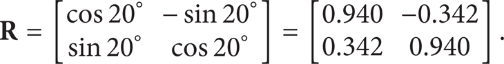
The coordinates {O₀} and {O₁} are shown in Figure 2. {O₀} is the fixed reference coordinate system, and {O₁} is attached to the upper arm of HHA. Referenced to the horizontal, the upward inclination of the upper arm is up about 20°.

Figure 2:

Structure of forearm in {O₀} and {O₁}.

The same point p is described in {O₀} and {O₁}: ${}^0\mathit{p}$ and ${}^1\mathit{p}$ have transformation relations as follows:

${}_{\mathrm{\hspace{0.17em}\hspace{0.17em}}}{}^{\mathrm{0}}\mathbf{p}=\mathbf{R}{}^{\mathrm{1}}\mathbf{p},$

(1)

where

$\mathbf{R}=\left[\begin{array}{cc}\text{cos}\mathrm{2}{\mathrm{0}}^{\circ }& -\text{sin}\mathrm{2}{\mathrm{0}}^{\circ }\\ \text{sin}\mathrm{2}{\mathrm{0}}^{\circ }& \text{cos}\mathrm{2}{\mathrm{0}}^{\circ }\end{array}\right]=\left[\begin{array}{cc}\mathrm{0.940}& -\mathrm{0.342}\\ \mathrm{0.342}& \mathrm{0.940}\end{array}\right].$

(2)

Under the assumption of the regular shape, smooth surface, and linear density steady of every components, the sketch of HHA in {O₀} and {O₁} is shown in Figure 2. The dot Q, O, G is the center of mass of the motors M1, M2, and M3 and their pedestals, respectively. The dot C, A, F is the center of mass of the slip tubes S1, S2, and S3, respectively. The lengths of AN and CM are both l₁, and the lengths of OQ, AB, RC, RB, CD, BC, EF, DE, ID, and FH are l₀, l₂, l₃, l₄, l₅, l₆, l₁₁, l₁₀, l₁₅, and l₃₀, respectively. The lengths of QC, OA, and GF are defined as x₁, x₂, and x₃, respectively.

In coordinates {O₁} and {O₀}, the position vectors of dot A and C are

$\begin{array}{c}{{}^{O_{\mathrm{1}}}\mathit{p}}_A={\left[\begin{array}{cc}{x}_{\mathrm{2}}& \mathrm{0}\end{array}\right]}^T,\hspace{1em}\hspace{1em}{{}^{O_{\mathrm{1}}}\mathit{p}}_C={\left[\begin{array}{cc}{x}_{\mathrm{1}}& l_{\mathrm{1}}\end{array}\right]}^T,\\ {{}^{O_{\mathrm{0}}}\mathit{p}}_A=\mathit{R}{\left[\begin{array}{cc}{x}_{\mathrm{2}}& \mathrm{0}\end{array}\right]}^T,\hspace{1em}\hspace{1em}{{}^{O_{\mathrm{0}}}\mathit{p}}_C=\mathit{R}{\left[\begin{array}{cc}{x}_{\mathrm{1}}& l_{\mathrm{1}}\end{array}\right]}^T.\end{array}$

(3)

As shown in Figure 2, β is the angle between CD and the axis X₁. α is the angle between AB and axis X₁. The HHA is on the initial state when β = 0.

Define

$\begin{array}{c}\mathrm{\Delta }x=x_{\mathrm{1}}-x_{\mathrm{2}},\hspace{1em}\hspace{1em}{l}_{\mathrm{7}}=l_{\mathrm{15}}-x_{\mathrm{3}},\hspace{1em}\hspace{1em}{l}_{\mathrm{8}}=\sqrt{l_{\mathrm{1}}^{\mathrm{2}}+{\mathrm{\Delta }}^{\mathrm{2}}x},\\ l_{\mathrm{9}}=\sqrt{\mathrm{4}{l}_{\mathrm{6}}^{\mathrm{2}}{l}_{\mathrm{8}}^{\mathrm{2}}-{\left(l_{\mathrm{8}}^{\mathrm{2}}+l_{\mathrm{6}}^{\mathrm{2}}-l_{\mathrm{2}}^{\mathrm{2}}\right)}^{\mathrm{2}}},\hspace{1em}\hspace{1em}{l}_{\mathrm{16}}=\sqrt{l_{\mathrm{10}}^{\mathrm{2}}+l_{\mathrm{7}}^{\mathrm{2}}},\\ l_{\mathrm{20}}=\sqrt{l_{\mathrm{10}}^{\mathrm{2}}+l_{\mathrm{16}}^{\mathrm{2}}-l_{\mathrm{11}}^{\mathrm{2}}},\hspace{1em}\hspace{1em}{l}_{\mathrm{22}}=\sqrt{l_{\mathrm{11}}^{\mathrm{2}}+l_{\mathrm{16}}^{\mathrm{2}}-l_{\mathrm{10}}^{\mathrm{2}}},\\ \mathbf{\Omega }={\left[\begin{array}{cc}\text{cos}\alpha & -\text{sin}\alpha \end{array}\right]}^T,\hspace{1em}\hspace{1em}\stackrel{-}{\mathbf{\Omega }}={\left[\begin{array}{cc}\text{sin}\alpha & \text{cos}\alpha \end{array}\right]}^T,\\ {\mathrm{\Theta }}_{\mathrm{1}}={\left[\begin{array}{cc}-\text{sin}\beta & \text{cos}\beta \end{array}\right]}^T,\hspace{1em}\hspace{1em}\stackrel{-}{\mathrm{\Theta }}={\left[\begin{array}{cc}\text{cos}\beta & \text{sin}\beta \end{array}\right]}^T,\\ {\mathrm{\Phi }}_{\mathrm{1}}={\left[\begin{array}{cc}\text{cos}{\theta }_{\mathrm{1}}& \text{sin}{\theta }_{\mathrm{1}}\end{array}\right]}^T,\hspace{1em}\hspace{1em}{\mathrm{\Phi }}_{\mathrm{2}}={\left[\begin{array}{cc}\text{cos}{\theta }_{\mathrm{2}}& -\text{sin}{\theta }_{\mathrm{2}}\end{array}\right]}^T,\\ {\mathbf{e}}_{\mathrm{1}}={\left[\begin{array}{cc}\mathrm{1}& \mathrm{0}\end{array}\right]}^T,\hspace{1em}\hspace{1em}{\mathbf{e}}_{\mathrm{2}}={\left[\begin{array}{cc}\mathrm{0}& \mathrm{1}\end{array}\right]}^T,\\ \mathrm{\Theta }=\left[\begin{array}{cc}\stackrel{-}{\mathrm{\Theta }}& {\mathrm{\Theta }}_{\mathrm{1}}\end{array}\right],\hspace{1em}\hspace{1em}{\mathbf{L}}_{\mathrm{34}}=\left[\begin{array}{cc}{l}_{\mathrm{3}}& l_{\mathrm{4}}\end{array}\right],\hspace{1em}\hspace{1em}\mathbf{E}=\left[\begin{array}{cc}{\mathbf{e}}_{\mathrm{1}}& {\mathbf{e}}_{\mathrm{2}}\end{array}\right].\end{array}$

(4)

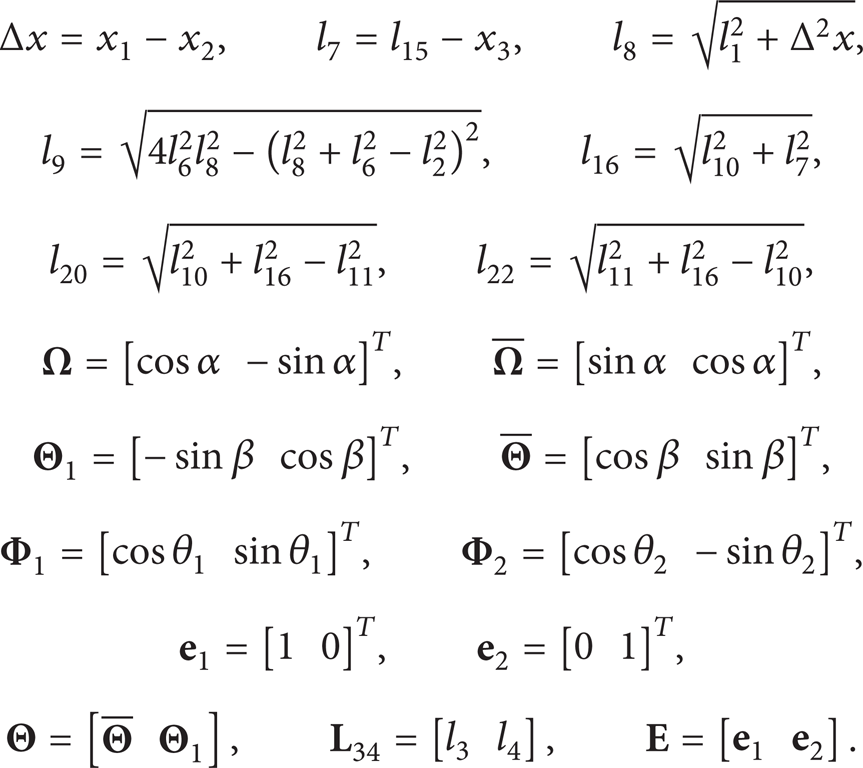
As shown in Figure 2, the angles β and α can be described as follows:

$\begin{array}{c}\beta ={\beta }_{\mathrm{1}}+{\beta }_{\mathrm{2}}+{\beta }_{\mathrm{3}}-\frac{\pi }{\mathrm{2}},\\ {\beta }_{\mathrm{1}}=\text{arctg}\left(\frac{l_{\mathrm{1}}}{\mathrm{\Delta }x}\right),\hspace{1em}\hspace{1em}{\beta }_{\mathrm{3}}=\text{arctg}\left(\frac{l_{\mathrm{4}}}{l_{\mathrm{1}}}\right),\\ {\beta }_{\mathrm{2}}=\text{arccos}\left(\frac{l_{\mathrm{8}}^{\mathrm{2}}+l_{\mathrm{6}}^{\mathrm{2}}-l_{\mathrm{2}}^{\mathrm{2}}}{\mathrm{2}{l}_{\mathrm{6}}{l}_{\mathrm{8}}}\right),\\ \alpha =\text{arctg}\frac{l_{\mathrm{1}}-{\mathbf{L}}_{\mathrm{34}}\stackrel{-}{\mathrm{\Theta }}}{\mathrm{\Delta }x-{\mathbf{L}}_{\mathrm{34}}{\mathrm{\Theta }}_{\mathrm{1}}}.\end{array}$

(5)

The angle θ₁ which is the angle between DE and CD and the angle θ₂ which is the angle between EF and GF can be described as follows:

$\begin{array}{c}{\theta }_{\mathrm{1}}=\text{arccos}\left(-\frac{l_{\mathrm{7}}}{l_{\mathrm{16}}}\right)-\text{arccos}\left(\frac{l_{\mathrm{20}}^{\mathrm{2}}}{\left(\mathrm{2}{l}_{\mathrm{10}}{l}_{\mathrm{16}}\right)}\right),\\ {\theta }_{\mathrm{2}}=\text{arccos}\left(\frac{l_{\mathrm{7}}}{l_{\mathrm{16}}}\right)-\text{arccos}\left(\frac{l_{\mathrm{22}}^{\mathrm{2}}}{\left(\mathrm{2}{l}_{\mathrm{11}}{l}_{\mathrm{16}}\right)}\right).\end{array}$

(6)

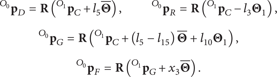
In coordinates {O₀}, the position vectors of D, R, G, and F can be described as follows:

$\begin{array}{c}{}^{O_{\mathrm{0}}}{\mathbf{p}}_D=\mathbf{R}\left({}^{O_{\mathrm{1}}}{\mathbf{p}}_C+\hspace{0.17em}{l}_{\mathrm{5}}\stackrel{-}{\mathrm{\Theta }}\right),\hspace{1em}\hspace{1em}{}^{O_{\mathrm{0}}}{\mathbf{p}}_R=\mathbf{R}\left({}^{O_{\mathrm{1}}}{\mathbf{p}}_C-\hspace{0.17em}{l}_{\mathrm{3}}{\mathrm{\Theta }}_{\mathrm{1}}\right),\\ {}^{O_{\mathrm{0}}}{\mathbf{p}}_G=\mathbf{R}\left({}^{O_{\mathrm{1}}}{\mathbf{p}}_C+\left(l_{\mathrm{5}}-l_{\mathrm{15}}\right)\stackrel{-}{\mathrm{\Theta }}+l_{\mathrm{10}}{\mathrm{\Theta }}_{\mathrm{1}}\right),\\ {}^{O_{\mathrm{0}}}{\mathbf{p}}_F=\mathbf{R}\left({}^{O_{\mathrm{1}}}{\mathbf{p}}_G+\hspace{0.17em}{x}_{\mathrm{3}}\stackrel{-}{\mathrm{\Theta }}\right).\end{array}$

(7)

Ax, Bx, Cx, and Dx are arbitrary dots of AB, RB, RC, and CD. In coordinates {O₀}, their position vectors are

$\begin{array}{c}{}^{O_{\mathrm{0}}}{\mathbf{p}}_{Ax}=\mathbf{R}\left({}^{O_{\mathrm{1}}}{\mathit{p}}_A+\hspace{0.17em}x\mathit{\Omega }\right),\hspace{1em}\hspace{1em}\mathrm{0}\le x\le l_{\mathrm{2}},\\ {}^{O_{\mathrm{0}}}{\mathbf{p}}_{Bx}=\mathbf{R}\left({}^{O_{\mathrm{1}}}{\mathbf{p}}_R-\hspace{0.17em}x\stackrel{-}{\mathrm{\Theta }}\right),\hspace{1em}\hspace{1em}\mathrm{0}\le x\le l_{\mathrm{4}},\\ {}^{O_{\mathrm{0}}}{\mathbf{p}}_{Cx}=\mathbf{R}\left({}^{O_{\mathrm{1}}}{\mathbf{p}}_C-\hspace{0.17em}x{\mathrm{\Theta }}_{\mathrm{1}}\right),\hspace{1em}\hspace{1em}\mathrm{0}\le x\le l_{\mathrm{3}},\\ {}^{O_{\mathrm{0}}}{\mathbf{p}}_{Dx}=\mathbf{R}\left({}^{O_{\mathrm{1}}}{\mathbf{p}}_C+\hspace{0.17em}x\stackrel{-}{\mathrm{\Theta }}\right),\hspace{1em}\hspace{1em}\mathrm{0}\le x\le l_{\mathrm{5}}.\end{array}$

(8)

Mx and Nx are arbitrary dots in CN and AN. In coordinates {O₀}, their position vectors are

$\begin{array}{c}{}^{O_{\mathrm{0}}}{\mathbf{p}}_{Mx}=\mathbf{R}\left({}^{O_{\mathrm{1}}}{\mathbf{p}}_A-\hspace{0.17em}x{\mathbf{e}}_{\mathrm{1}}\right),\hspace{1em}\hspace{1em}\mathrm{0}<x<l_{\mathrm{1}},\\ {}^{O_{\mathrm{0}}}{\mathbf{p}}_{Nx}=\mathbf{R}\left({}^{O_{\mathrm{1}}}{\mathbf{p}}_C+\hspace{0.17em}x{\mathbf{e}}_{\mathrm{1}}\right),\hspace{1em}\hspace{1em}\mathrm{0}\le x\le l_{\mathrm{1}}.\end{array}$

(9)

Gx, Fx, and Ex are arbitrary dots in HF, EF, and DE. In coordinates {O₀}, their position vectors are

$\begin{array}{c}{}^{O_{\mathrm{0}}}{\mathbf{p}}_{Gx}=\mathbf{R}\left({}^{O_{\mathrm{1}}}{\mathbf{p}}_F-\hspace{0.17em}x\stackrel{-}{\mathrm{\Theta }}\right),\hspace{1em}\hspace{1em}\mathrm{0}<x<l_{\mathrm{30}},\\ {}^{O_{\mathrm{0}}}{\mathbf{p}}_{Fx}=\mathbf{R}\left({}_{\mathrm{\hspace{0.17em}\hspace{0.17em}}}{}^{O_{\mathrm{1}}}{\mathbf{p}}_F+\hspace{0.17em}x\mathrm{\Theta }{\mathrm{\Phi }}_{\mathrm{2}}\right),\hspace{1em}\hspace{1em}\mathrm{0}\le x\le l_{\mathrm{11}},\\ {}^{O_{\mathrm{0}}}{\mathbf{p}}_{Ex}=\mathbf{R}\left({}_{\mathrm{\hspace{0.17em}\hspace{0.17em}}}{}^{O_{\mathrm{1}}}{\mathbf{p}}_D+\hspace{0.17em}x\mathrm{\Theta }{\mathrm{\Phi }}_{\mathrm{1}}\right),\hspace{1em}\hspace{1em}\mathrm{0}\le x\le l_{\mathrm{10}}.\end{array}$

(10)

2.2. Analysis and Reference Trajectory of Throwing Process

A complete throwing process of HHA in a cycle consists of three stages: HHA raising from initial state stage, HHA waiting for the load stage, and HHA throwing the load out stage. Whether the object can be thrown at a certain position and a certain speed is a key part in the complete throwing process, and obtaining the corresponding reference signal is considered as a difficult problem.

To obtain the corresponding reference signal, a method we proposed is shown as follows. Firstly, the changing curve of HHA elbow joint angle, wrist joint angle, and time should be found by analyzing the throwing process of man's arm, respectively, and then the changing curve of Δx, x₃ and time can be found through formula (5) and (6), respectively. By planning the motion of S1 and S2, we can get the changing curve of x₁, x₂, x₃, and time, respectively.

To study the man's throwing process in detail, a camera is used to get the video image of raising and throwing process. After processing by MATLAB and Photoshop, the video image can be divided into four parts: the raising of forearm, the putting down of forearm, the raising of hand, and the putting down of hand. Define the beginning time of raising process at 0 seconds and the beginning time of throwing process at 1.5 seconds; the video image processing results are shown in Figure 3.

Figure 3:

Video image processing results of complete throwing process. (a) Forearm raising, (b) forearm putting down, (c) hand raising, and (d) hand putting down video image processing result.

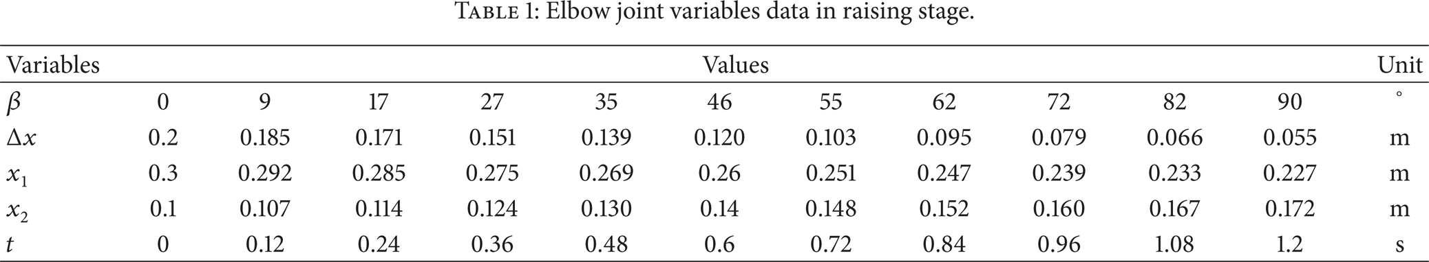
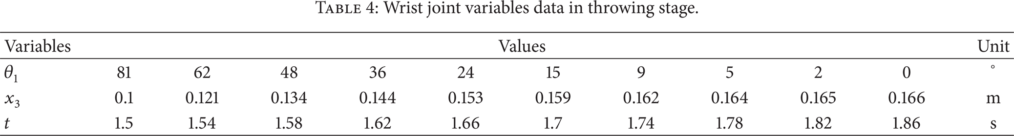
Considering the structure of the elbow joint and energy saving, the Δx can be produced by the following ways: when the forearm is raising, S1 and S2 move close to each other; when the forearm is putting down, S1 and S2 move away from each other. Then, the relationship between variables β, Δx, x₁, x₂, and time are shown in Tables 1 and 2; the relationship between variables θ₁, x₃, and time are shown in Tables 3 and 4, respectively. Processing the data in Tables 1–4 by MATLAB CFtool, we get the changing curve of x₁, x₂, x₃ time in a cycle as shown in Figure 4 and their fragment expressions are given as follows:

$\begin{array}{c}{x}_{\mathrm{1}}=\{\begin{array}{cc}\mathrm{0.01}{t}^{\mathrm{2}}-\mathrm{0.073}t+\mathrm{0.3},\hfill & \mathrm{0}\le t<\mathrm{1.2}\text{s}\hfill \\ \mathrm{0.227},\hfill & \mathrm{1.2}\text{s}\le t\le \mathrm{1.5}\text{s}\hfill \\ -\mathrm{0.099}{t}^{\mathrm{2}}+\mathrm{0.468}t-\mathrm{0.252},\hfill & \mathrm{1.5}\text{s}\le t<\mathrm{2.3}\text{s},\hfill \end{array}\\ x_{\mathrm{2}}=\{\begin{array}{cc}-\mathrm{0.009}{t}^{\mathrm{2}}+\mathrm{0.071}t+\mathrm{0.1},\hfill & \mathrm{0}\le t<\mathrm{1.2}\text{s}\hfill \\ \mathrm{0.172},\hfill & \mathrm{1.2}\text{s}\le t\le \mathrm{1.5}\text{s}\hfill \\ \mathrm{0.099}{t}^{\mathrm{2}}-\mathrm{0.468}t+\mathrm{0.649},\hfill & \mathrm{1.5}\text{s}\le t\le \mathrm{2.3}\text{s},\hfill \end{array}\\ x_{\mathrm{3}}=\{\begin{array}{cc}-\mathrm{0.027}{t}^{\mathrm{2}}-\mathrm{0.032}t+\mathrm{0.166},\hfill & \mathrm{0}\le t<\mathrm{1.08}\text{s}\hfill \\ \mathrm{0.1},\hfill & \mathrm{1.08}\text{s}\le t\le \mathrm{1.5}\text{s}\hfill \\ \mathrm{0.2}{e}^{-\mathrm{0.358}\left(x-\mathrm{1.5}\right)}-\mathrm{0.1}{e}^{-\mathrm{6.45}\left(x-\mathrm{1.5}\right)},\hfill & \mathrm{1.5}\text{s}\le t<\mathrm{1.86}\text{s}\hfill \\ \mathrm{0.166},\hfill & \mathrm{1.86}\text{s}\le t\le \mathrm{2.3}\text{s}.\hfill \end{array}\end{array}$

(11)

Table 1:

Elbow joint variables data in raising stage.

Variables	Values											Unit
β	0	9	17	27	35	46	55	62	72	82	90	°
Δx	0.2	0.185	0.171	0.151	0.139	0.120	0.103	0.095	0.079	0.066	0.055	m
x 1	0.3	0.292	0.285	0.275	0.269	0.26	0.251	0.247	0.239	0.233	0.227	m
x 2	0.1	0.107	0.114	0.124	0.130	0.14	0.148	0.152	0.160	0.167	0.172	m
t	0	0.12	0.24	0.36	0.48	0.6	0.72	0.84	0.96	1.08	1.2	s

Table 2:

Elbow joint variables data in throwing stage.

Variables	Values											Unit
β	90	70	57	43	33	24	15	9	5	2	0	°
Δx	0.055	0.082	0.102	0.125	0.142	0.159	0.174	0.185	0.192	0.197	0.2	m
x 1	0.227	0.241	0.251	0.262	0.271	0.279	0.287	0.292	0.296	0.298	0.3	m
x 2	0.172	0.159	0.149	0.137	0.129	0.120	0.113	0.107	0.104	0.101	0.1	m
t	1.5	1.58	1.66	1.74	1.822	1.9	1.98	2.06	2.14	2.22	2.3	s

Table 3:

Wrist joint variables data in raising stage.

Variables	Values										Unit
θ1	0	10	17	27	36	46	53	62	73	81	°
x 3	0.166	0.162	0.157	0.151	0.144	0.137	0.129	0.120	0.11	0.1	m
t	0	0.12	0.24	0.36	0.48	0.6	0.72	0.84	0.96	1.08	s

Table 4:

Wrist joint variables data in throwing stage.

Variables	Values										Unit
θ1	81	62	48	36	24	15	9	5	2	0	°
x 3	0.1	0.121	0.134	0.144	0.153	0.159	0.162	0.164	0.165	0.166	m
t	1.5	1.54	1.58	1.62	1.66	1.7	1.74	1.78	1.82	1.86	s

Figure 4:

Position motion of the slip tubes. (a) The motion of S1, (b) the motion of S2, and (c) the motion of S3.

3. Dynamic Modeling for HHA

In this section, the dynamic model of the HHA is derived. The Lagrange formalism used for the serial-parallel mechanism can be written as follows:

$\frac{d}{dt}\left(\frac{\partial L}{\partial \dot{\mathbf{q}}}\right)-\frac{\partial L}{\partial \mathbf{q}}=\mathit{\tau },$

(12)

where L = V – P is the Lagrange function, K and P are the kinetic and potential energy functions, respectively, $\mathit{q}={\left[\begin{array}{ccc}{q}_1& q_2& q_3\end{array}\right]}^T$ , $\dot{\mathit{q}}={\left[\begin{array}{ccc}{\dot{q}}_1& {\dot{q}}_2& {\dot{q}}_3\end{array}\right]}^T$ are the vectors of the slip tubes position and velocity τ^{3 × 3} is the vector of the corresponding control input forces.

3.1. The Computing for Kinetic and Potential Energy of Every Component

The total kinetic and potential energy of movers P1, P2, and P3 is given, respectively, as

$\begin{array}{c}{V}_{\mathrm{1}}=\frac{\mathrm{1}}{\mathrm{2}}{\rho }_{\mathrm{1}}{\int }_{\mathrm{0}}^{l_{\mathrm{1}}}\left({}^{O_{\mathrm{0}}}{\dot{\mathbf{p}}}_{Mx}^T{}^{O_{\mathrm{0}}}{\dot{\mathbf{p}}}_{Mx}+{}^{O_{\mathrm{0}}}{\dot{\mathbf{p}}}_{Nx}^T{}^{O_{\mathrm{0}}}{\dot{\mathbf{p}}}_{Nx}\right)\text{d}x,\\ P_{\mathrm{1}}={\rho }_{\mathrm{1}}g{\int }_{\mathrm{0}}^{l_{\mathrm{1}}}\left({\mathbf{e}}_{\mathrm{2}}^T{}^{O_{\mathrm{0}}}{\mathbf{p}}_{Mx}+{\mathbf{e}}_{\mathrm{2}}^T{}^{O_{\mathrm{0}}}{\mathbf{p}}_{Nx}\right)\text{d}x,\\ V_{\mathrm{2}}=\frac{\mathrm{1}}{\mathrm{2}}{\rho }_{\mathrm{1}}{\int }_{\mathrm{0}}^{l_{\mathrm{30}}}{}^{O_{\mathrm{0}}}{\dot{\mathbf{p}}}_{Gx}^T{}^{O_{\mathrm{0}}}{\dot{\mathbf{p}}}_{Gx}\text{d}x,\\ P_{\mathrm{2}}={\rho }_{\mathrm{1}}g{\int }_{\mathrm{0}}^{l_{\mathrm{30}}}{\mathbf{e}}_{\mathrm{2}}^T{}^{O_{\mathrm{0}}}{\mathbf{p}}_{Gx}\text{d}x,\end{array}$

(13)

where ρ₁ is the linear density of P1, P2, and P3.

The kinetic and potential energy of part CD and wrist handspike is given, respectively, as

$\begin{array}{c}{V}_{\mathrm{3}}=\frac{\mathrm{1}}{\mathrm{2}}{\rho }_{\mathrm{2}}{\int }_{\mathrm{0}}^{l_{\mathrm{5}}}{}^{O_{\mathrm{0}}}{\dot{\mathbf{p}}}_{Dx}^T{}^{O_{\mathrm{0}}}{\dot{\mathbf{p}}}_{Dx}\text{d}x,\\ P_{\mathrm{3}}={\rho }_{\mathrm{2}}g{\int }_{\mathrm{0}}^{l_{\mathrm{5}}}{\mathbf{e}}_{\mathrm{2}}^T{}^{O_{\mathrm{0}}}{\mathbf{p}}_{Dx}\text{d}x,\\ V_{\mathrm{4}}=\frac{\mathrm{1}}{\mathrm{2}}{\rho }_{\mathrm{3}}{\int }_{\mathrm{0}}^{l_{\mathrm{10}}}{}^{O_{\mathrm{0}}}{\dot{\mathbf{p}}}_{Ex}^T{}^{O_{\mathrm{0}}}{\dot{\mathbf{p}}}_{Ex}\text{d}x,\\ P_{\mathrm{4}}={\rho }_{\mathrm{3}}g{\int }_{\mathrm{0}}^{l_{\mathrm{10}}}{\mathbf{e}}_{\mathrm{2}}^T{}^{O_{\mathrm{0}}}{\mathbf{p}}_{Ex}\text{d}x,\end{array}$

(14)

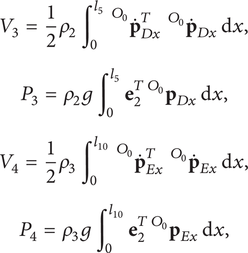
where ρ₂ and ρ₃ are the linear density of CD and wrist handspike, respectively.

The kinetic and potential energy of parts AB, BR, RC, and EF of forearm pedestal is given, respectively, as

$\begin{array}{c}{V}_{\mathrm{5}}=\frac{\mathrm{1}}{\mathrm{2}}{\rho }_{\mathrm{4}}{\int }_{\mathrm{0}}^{l_{\mathrm{2}}}{}^{O_{\mathrm{0}}}{\dot{\mathbf{p}}}_{Ax}^T{}^{O_{\mathrm{0}}}{\dot{\mathbf{p}}}_{Ax}\text{d}x,\\ P_{\mathrm{5}}={\rho }_{\mathrm{4}}g{\int }_{\mathrm{0}}^{l_{\mathrm{2}}}{\mathbf{e}}_{\mathrm{2}}^T{}^{O_{\mathrm{0}}}{\mathbf{p}}_{Ax}\text{d}x,\\ V_{\mathrm{6}}=\frac{\mathrm{1}}{\mathrm{2}}{\rho }_{\mathrm{4}}{\int }_{\mathrm{0}}^{l_{\mathrm{4}}}{}^{O_{\mathrm{0}}}{\dot{\mathbf{p}}}_{Bx}^T{}^{O_{\mathrm{0}}}{\dot{\mathbf{p}}}_{Bx}\text{d}x,\\ P_{\mathrm{6}}={\rho }_{\mathrm{4}}g{\int }_{\mathrm{0}}^{l_{\mathrm{4}}}{\mathbf{e}}_{\mathrm{2}}^T{}^{O_{\mathrm{0}}}{\mathbf{p}}_{Bx}\text{d}x,\\ V_{\mathrm{7}}=\frac{\mathrm{1}}{\mathrm{2}}{\rho }_{\mathrm{4}}{\int }_{\mathrm{0}}^{l_{\mathrm{3}}}{}^{O_{\mathrm{0}}}{\dot{\mathbf{p}}}_{Cx}^T{}^{O_{\mathrm{0}}}{\dot{\mathbf{p}}}_{Cx}\text{d}x,\\ P_{\mathrm{7}}={\rho }_{\mathrm{4}}g{\int }_{\mathrm{0}}^{l_{\mathrm{3}}}{\mathbf{e}}_{\mathrm{2}}^T{}^{O_{\mathrm{0}}}{\mathbf{p}}_{Cx}\text{d}x,\\ V_{\mathrm{8}}=\frac{\mathrm{1}}{\mathrm{2}}{\rho }_{\mathrm{4}}{\int }_{\mathrm{0}}^{l_{\mathrm{11}}}{}^{O_{\mathrm{0}}}{\dot{\mathbf{p}}}_{Fx}^T{}^{O_{\mathrm{0}}}{\dot{\mathbf{p}}}_{Fx}\text{d}x,\\ P_{\mathrm{8}}={\rho }_{\mathrm{4}}g{\int }_{\mathrm{0}}^{l_{\mathrm{11}}}{\mathbf{e}}_{\mathrm{2}}^T{}^{O_{\mathrm{0}}}{\mathbf{p}}_{Fx}\text{d}x,\end{array}$

(15)

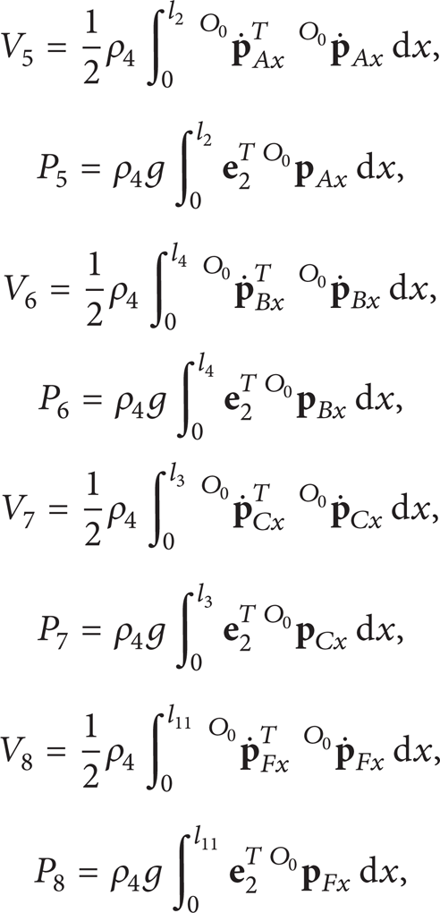
where ρ₂ is the linear density of AB, BR, RC, and EF.

The total kinetic and potential energy of motor M3 and its pedestal is given as

$V_{\mathrm{9}}=\frac{\mathrm{1}}{\mathrm{2}}{m}_{\mathrm{6}}{}^{O_{\mathrm{0}}}{\dot{\mathbf{p}}}_Q^T{}^{O_{\mathrm{0}}}{\dot{\mathbf{p}}}_Q,\hspace{1em}\hspace{1em}{P}_{\mathrm{9}}=m_{\mathrm{6}}g{\mathbf{e}}_{\mathrm{2}}^T{}^{O_{\mathrm{0}}}{\mathbf{p}}_Q,$

(16)

where m₉ is the mass of M3 and its pedestal.

3.2. The Dynamic Model of the HHA

The dynamics of the HHA can be written as

$\mathbf{M}\left(\mathbf{q}\right)\stackrel{‥}{\mathbf{q}}+\mathbf{C}\left(\mathbf{q},\dot{\mathbf{q}}\right)\dot{\mathbf{q}}+\mathbf{G}\left(\mathbf{q}\right)+{\mathit{\tau }}_d=\mathit{\tau },$

(17)

where $\mathbf{q},\mathrm{\hspace{0.17em}\hspace{0.17em}}\mathrm{\hspace{0.17em}\hspace{0.17em}}\dot{\mathbf{q}},\mathrm{\hspace{0.17em}\hspace{0.17em}}\mathrm{\hspace{0.17em}\hspace{0.17em}}\stackrel{‥}{\mathbf{q}}∊R^{\mathrm{3}}$ are the vectors of slip tubes position, velocity, and acceleration, respectively, $\mathbf{M}(\mathbf{q})={\mathbf{M}}_{\mathrm{0}}(\mathbf{q})+\mathrm{\Delta }\mathbf{M}(\mathbf{q})∊R^{\mathrm{3}\mathrm{\hspace{0.17em}\hspace{0.17em}}\times \mathrm{\hspace{0.17em}\hspace{0.17em}}\mathrm{3}}$ is a symmetric positive definite inertia matrix, $\mathbf{C}(\mathbf{q},\dot{\mathbf{q}})={\mathbf{C}}_{\mathrm{0}}(\mathbf{q},\dot{\mathbf{q}})+\mathrm{\Delta }\mathbf{C}(\mathbf{q},\dot{\mathbf{q}})\mathrm{\hspace{0.17em}\hspace{0.17em}}∊R^{\mathrm{3}\mathrm{\hspace{0.17em}\hspace{0.17em}}\times \mathrm{\hspace{0.17em}\hspace{0.17em}}\mathrm{3}}$ is the matrix of centripetal and coriolis force, $\mathbf{G}(\mathbf{q})={\mathbf{G}}_{\mathrm{0}}(\mathbf{q})+\mathrm{\Delta }\mathbf{G}(\mathbf{q})∊R^{\mathrm{3}}$ is the vector of gravitational force, τ _d ∊ R³ is the vector of generalized input due to external disturbance with $\parallel {\mathit{\tau }}_d\parallel \le d$ , and τ ∊ R³ is the input force vector. Here ${\mathbf{M}}_{\mathrm{0}}(\mathbf{q})$ , ${\mathbf{C}}_{\mathrm{0}}(\mathbf{q},\dot{\mathbf{q}})$ , and ${\mathbf{G}}_{\mathrm{0}}(\mathbf{q})$ are the nominal parts calculated by Lagrange method, where $\mathrm{\Delta }{\mathbf{M}}_{\mathrm{0}}(\mathbf{q})$ , $\mathrm{\Delta }{\mathbf{C}}_{\mathrm{0}}(\mathbf{q},\dot{\mathbf{q}})$ , and $\mathrm{\Delta }{\mathbf{G}}_{\mathrm{0}}(\mathbf{q})$ represent the perturbations in the system matrices. Then the dynamic model of HHA can be rewritten as

${\mathbf{M}}_{\mathrm{0}}\left(\mathbf{q}\right)\stackrel{‥}{\mathbf{q}}+{\mathbf{C}}_{\mathrm{0}}\left(\mathbf{q},\dot{\mathbf{q}}\right)\dot{\mathbf{q}}+{\mathbf{G}}_{\mathrm{0}}\left(\mathbf{q}\right)+{\mathit{\tau }}_d+\mathbf{F}\left(\mathbf{q},\dot{\mathbf{q}},\stackrel{‥}{\mathbf{q}}\right)=\mathit{\tau },$

(18)

where

$\mathbf{F}\left(\mathbf{q},\dot{\mathbf{q}},\stackrel{‥}{\mathbf{q}}\right)=\mathrm{\Delta }{\mathbf{M}}_{\mathrm{0}}\left(\mathbf{q}\right)\stackrel{‥}{\mathbf{q}}+\mathrm{\Delta }{\mathbf{C}}_{\mathrm{0}}\left(\mathbf{q},\dot{\mathbf{q}}\right)\dot{\mathbf{q}}+\mathrm{\Delta }{\mathbf{G}}_{\mathrm{0}}\left(\mathbf{q}\right)∊R^{\mathrm{3}}$

(19)

is the lumped system uncertainty and satisfies [9]

$\parallel \mathbf{F}\left(\mathbf{q},\dot{\mathbf{q}},\stackrel{‥}{\mathbf{q}}\right)\parallel \le b_{\mathrm{0}}+b_{\mathrm{1}}\parallel \mathbf{q}\parallel +b_{\mathrm{2}}{\parallel \dot{\mathbf{q}}\parallel }^{\mathrm{2}}.$

(20)

4. Fuzzy Self-Tuning Disturbance Decoupling Control (FSDDC) for HHA

In this section, the FSDDC for HHA is developed, which combines the advantages of the DDC and the FLC. First, the DDC for HHA is derived. Then, the FSDDC is proposed to establish the FLC for the proposed DDC.

4.1. Disturbance Decoupling Control (DDC) for HHA

DDC is a relatively new control design concept and a natural fit for the purpose of disturbance decoupling in robot systems. As it is applied to the control of the HHA system, the idea is that all the nonlinear, time-varying uncertainties and coupling terms are parts of the total disturbance and can be actively estimated using the extended state observer (ESO) and canceled in the control law, leading to roughly three single-input and single-output plants. In this section, three disturbance decoupling controllers are designed for HHA to do trajectory tracking.

The realistic model (18) can be reformulated as

$\begin{array}{c}\stackrel{‥}{\mathbf{q}}=-{{\mathbf{M}}_{\mathrm{0}}}^{-\mathrm{1}}\left({\mathbf{C}}_{\mathrm{0}}\dot{\mathbf{q}}+{\mathbf{G}}_{\mathrm{0}}+{\mathit{\tau }}_d+\mathbf{F}\right)+{{\mathbf{M}}_{\mathrm{0}}}^{-\mathrm{1}}\mathit{\tau }.\\ \text{Define}\mathrm{\hspace{0.17em}\hspace{0.17em}}{\left[b_{\mathrm{1}},b_{\mathrm{2}},b_{\mathrm{3}}\right]}^T=\mathrm{diag}\left({{\mathbf{M}}_{\mathrm{0}}}^{-\mathrm{1}}\right)\mathrm{\hspace{0.17em}\hspace{0.17em}}\text{and}\mathrm{\hspace{0.17em}\hspace{0.17em}}\mathbf{e}={\mathbf{q}}_d-\mathbf{q},\end{array}$

(21)

where ${\mathbf{q}}_d={\left[\begin{array}{ccc}{q}_{d\mathrm{1}}& q_{d\mathrm{2}}& q_{d\mathrm{3}}\end{array}\right]}^T$ is the desired trajectory.

The HHA system can be formed by a set of coupled equations with predetermined input-output parings:

$\begin{array}{c}{\stackrel{‥}{q}}_{\mathrm{1}}=p_{\mathrm{1}}\left(\dot{\mathbf{q}},\mathbf{q},\mathit{\tau },{\tau }_{d\mathrm{1}},{\mathbf{F}}_{\mathrm{1}}\right)+b_{\mathrm{1}}{\tau }_{\mathrm{1}},\\ {\stackrel{‥}{q}}_{\mathrm{2}}=p_{\mathrm{2}}\left(\dot{\mathbf{q}},\mathbf{q},\mathit{\tau },{\tau }_{d\mathrm{2}},{\mathbf{F}}_{\mathrm{2}}\right)+b_{\mathrm{2}}{\tau }_{\mathrm{2}},\\ {\stackrel{‥}{q}}_{\mathrm{3}}=p_{\mathrm{3}}\left(\dot{\mathbf{q}},\mathbf{q},\mathit{\tau },{\tau }_{d\mathrm{3}},{\mathbf{F}}_{\mathrm{3}}\right)+b_{\mathrm{3}}{\tau }_{\mathrm{3}}.\end{array}$

(22)

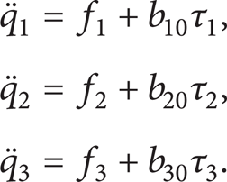
Define the total disturbance of each loop as

$f_i=p_i\left(\dot{\mathbf{q}},\mathbf{q},\mathit{\tau },{\tau }_{di},{\mathbf{F}}_i\right)+\left(b_i-b_{i\mathrm{0}}\right){\tau }_i,\hspace{1em}i=\mathrm{1},\mathrm{2},\mathrm{3},$

(23)

where b_i0 is the approximate value of b _i , f _i represents the combined effect of internal dynamics and external disturbances in the ith loop, including the cross-channel interference. Then (22) can be written as

$\begin{array}{c}{\stackrel{‥}{q}}_{\mathrm{1}}=f_{\mathrm{1}}+b_{\mathrm{10}}{\tau }_{\mathrm{1}},\\ {\stackrel{‥}{q}}_{\mathrm{2}}=f_{\mathrm{2}}+b_{\mathrm{20}}{\tau }_{\mathrm{2}},\\ {\stackrel{‥}{q}}_{\mathrm{3}}=f_{\mathrm{3}}+b_{\mathrm{30}}{\tau }_{\mathrm{3}}.\end{array}$

(24)

Now, the HHA system has been decoupled to a three-loop system as shown in Figure 5. Then an ADRC based SISO controller can be designed for each loop independently. The task of ADRC comes down to a critical subtask: estimate f _i in real time. The estimation problem of f _i leads us to a unique state observer known as the extended state observer (ESO).

Figure 5:

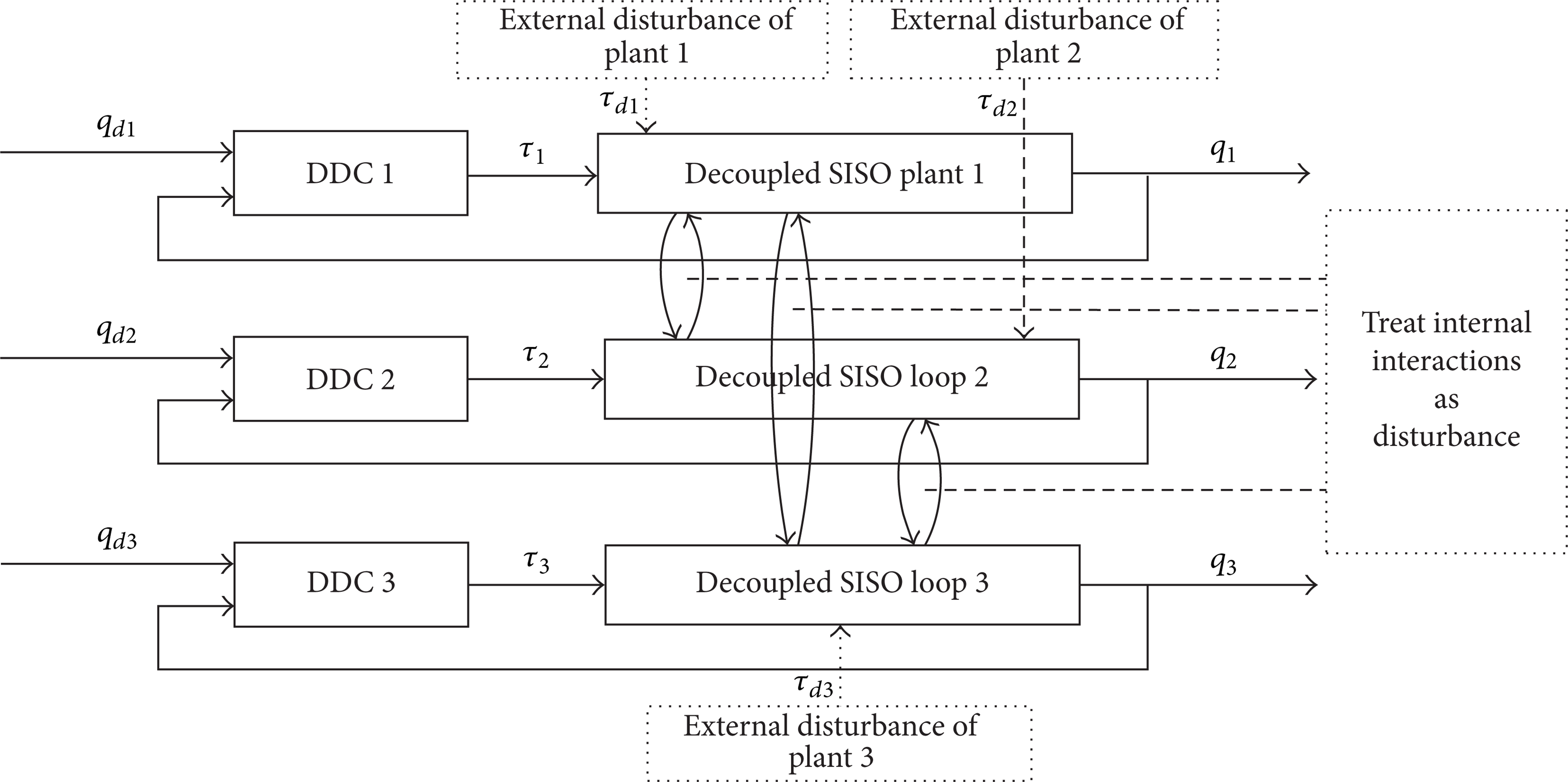
Diagram of the DDC for HHA.

Considering the first loop, the structure of DDC in first loop is given in Figure 6.

Figure 6:

The structure of DDC for first loop.

Let x₁₁ = q₁, $x_{\mathrm{12}}={\dot{q}}_{\mathrm{1}}$ , x₁₃ = f₁, which is added as an extended state. Assume f₁ is differentiable, and ${\dot{f}}_{\mathrm{1}}=h$ . The augmented model of (24) is

$\begin{array}{c}{\dot{x}}_{\mathrm{11}}=x_{\mathrm{12}},\hspace{1em}\hspace{1em}{\dot{x}}_{\mathrm{12}}=x_{\mathrm{13}}+b_{\mathrm{10}}{\tau }_{\mathrm{1}},\\ {\dot{x}}_{\mathrm{13}}=h_{\mathrm{1}},\hspace{1em}\hspace{1em}{q}_{\mathrm{1}}=x_{\mathrm{11}}.\end{array}$

(25)

Letting ${\mathbf{x}}_{\mathrm{1}}={\left[\begin{array}{ccc}{x}_{\mathrm{11}}& x_{\mathrm{12}}& x_{\mathrm{13}}\end{array}\right]}^T$ , the augmented state space form of (25) is

${\dot{\mathbf{x}}}_{\mathrm{1}}={\mathbf{A}}_{\mathrm{1}}\mathbf{x}+{\mathbf{B}}_{\mathrm{1}}{\tau }_{\mathrm{1}}+{\mathbf{E}}_{\mathrm{1}}{h}_{\mathrm{1}},\hspace{1em}\hspace{1em}{q}_{\mathrm{1}}={\mathbf{C}}_{\mathrm{1}}{\mathbf{x}}_{\mathrm{1}},$

(26)

where

$\begin{array}{c}{\mathbf{A}}_{\mathrm{1}}=\left[\begin{array}{ccc}\mathrm{0}& \mathrm{1}& \mathrm{0}\\ \mathrm{0}& \mathrm{0}& \mathrm{1}\\ \mathrm{0}& \mathrm{0}& \mathrm{0}\end{array}\right],\hspace{1em}\hspace{1em}{\mathbf{B}}_{\mathrm{1}}=\left[\begin{array}{c}\mathrm{0}\\ b_{\mathrm{10}}\\ \mathrm{0}\end{array}\right],\\ {\mathbf{C}}_{\mathrm{1}}={\left[\begin{array}{c}\mathrm{1}\\ \mathrm{0}\\ \mathrm{0}\end{array}\right]}^T,\hspace{1em}\hspace{1em}{\mathbf{E}}_{\mathrm{1}}=\left[\begin{array}{c}\mathrm{0}\\ \mathrm{0}\\ \mathrm{1}\end{array}\right].\end{array}$

(27)

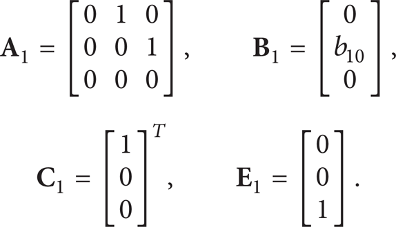
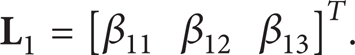
The state observer denoted as the linear extended state observer (LESO) of (26) is constructed as

${\dot{\mathbf{z}}}_{\mathrm{1}}={\mathbf{A}}_{\mathrm{1}}+{\mathbf{B}}_{\mathrm{1}}{\tau }_{\mathrm{1}}+{\mathbf{L}}_{\mathrm{1}}\left(q_{\mathrm{1}}-z_{\mathrm{11}}\right),\hspace{1em}\hspace{1em}{\widehat{q}}_{\mathrm{1}}=\mathbf{C}{\mathbf{z}}_{\mathrm{1}},$

(28)

where L₁ is the observer gain vector:

${\mathbf{L}}_{\mathrm{1}}={\left[\begin{array}{ccc}{\beta }_{\mathrm{11}}& {\beta }_{\mathrm{12}}& {\beta }_{\mathrm{13}}\end{array}\right]}^T.$

(29)

With the state observer properly designed, z₁₁, z₁₂, and z₁₃ closely track q₁, ${\dot{q}}_{\mathrm{1}}$ , and f₁, respectively. The controller is given by

${\tau }_{\mathrm{1}}=\frac{-z_{\mathrm{13}}+{\tau }_{\mathrm{10}}}{b_{\mathrm{10}}}.$

(30)

Ignoring the estimation error in z₁₃ to f₁, the plant is reduced to a unit gain double integrator,

${\stackrel{‥}{q}}_{\mathrm{1}}=\left(f_{\mathrm{1}}-z_{\mathrm{13}}\right)+{\tau }_{\mathrm{10}}\approx {\tau }_{\mathrm{10}},$

(31)

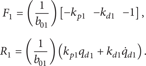
which can be easily controlled by a linear state error feedback (LSEF) controller:

${\tau }_{\mathrm{10}}=k_{p\mathrm{1}}\left({q_d}_{\mathrm{1}}-z_{\mathrm{11}}\right)+k_{d\mathrm{1}}\left({\dot{q}}_{d\mathrm{1}}-z_{\mathrm{12}}\right),$

(32)

where q_d1 is the desired trajectory of S1. Then the total control law of first loop is found as

${\tau }_{\mathrm{1}}=\frac{k_{p\mathrm{1}}\left({q_d}_{\mathrm{1}}-z_{\mathrm{11}}\right)+k_{d\mathrm{1}}\left({\dot{q}}_{d\mathrm{1}}-z_{\mathrm{12}}\right)-z_{\mathrm{13}}}{b_{\mathrm{10}}}.$

(33)

In order to simplify the tuning of ADRC parameters, a parameter tuning method of the LESO is proposed in [24]; with using the pole placement technique, all the observer poles are at – ω₀₁, making ω₀₁ the only tuning parameter for the LESO. That is

${\mathbf{L}}_{\mathrm{1}}={\left[\begin{array}{ccc}{\beta }_{\mathrm{11}}& {\beta }_{\mathrm{12}}& {\beta }_{\mathrm{13}}\end{array}\right]}^T=\left[\begin{array}{ccc}\mathrm{3}{\omega }_{\mathrm{01}}& \mathrm{3}{\omega }_{\mathrm{01}}^{\mathrm{2}}& {\omega }_{\mathrm{01}}^{\mathrm{3}}\end{array}\right],$

(34)

where ω₀₁ is the bandwidth of the LESO 1. This makes LADRC only have three tuning parameters ω₀₁, k_p1, and k_d1, compared to traditional ADRC controller.

4.2. Stability

Theorem 1. Assuming h₁ is bounded, the LESO is bounded-input bounded-output (BIBO) stable.

Proof. Let e_{1, i} = x_{1, i} – z_{1, i}, i = 1, 2, 3, and combine (28) and (29) and subtract it from (26); the error equation can be written as

${\dot{\mathbf{e}}}_{\mathrm{1}}={\mathbf{A}}_{e\mathrm{1}}{\mathbf{e}}_{\mathrm{1}}+{\mathbf{E}}_{\mathrm{1}}{h}_{\mathrm{1}},$

(35)

where

${\mathbf{A}}_{e\mathrm{1}}={\mathbf{A}}_{\mathrm{1}}-{\mathbf{L}}_{\mathrm{1}}{\mathbf{C}}_{\mathrm{1}}=\left[\begin{array}{ccc}-\mathrm{3}{\omega }_{\mathrm{01}}& \mathrm{1}& \mathrm{0}\\ -\mathrm{3}{\omega }_{\mathrm{01}}^{\mathrm{2}}& \mathrm{0}& \mathrm{1}\\ -{\omega }_{\mathrm{01}}^{\mathrm{3}}& \mathrm{0}& \mathrm{0}\end{array}\right],$

(36)

and E is defined in (26). The characteristic polynomial of A_e1 is

${\lambda }_{\mathrm{1}}\left(s\right)=s^{\mathrm{3}}+\mathrm{3}{\omega }_{\mathrm{01}}{s}^{\mathrm{2}}+\mathrm{3}{\omega }_{\mathrm{01}}^{\mathrm{2}}s+{\omega }_{\mathrm{01}}^{\mathrm{3}}.$

(37)

Letting ω₀₁ > 0, it is obvious the roots of the characteristic polynomial of A_e1 are all in the left plane and h₁ is bounded; we can draw the conclusion that the LESO 1 is bounded-input bounded-output (BIBO) stable.

Theorem 2. Assuming h₁ and q_d1 are bounded, the DDC 1 design from (28) to (33) yields a BIBO stable closed-loop system.

Proof. From (30) and (33), a state feedback equation can be described as

${\tau }_{\mathrm{1}}=\frac{k_{p\mathrm{1}}\left({q_d}_{\mathrm{1}}-z_{\mathrm{11}}\right)+k_{d\mathrm{1}}\left({\dot{q}}_{d\mathrm{1}}-z_{\mathrm{12}}\right)-z_{\mathrm{13}}}{b_{\mathrm{01}}}=F_{\mathrm{1}}{\mathbf{z}}_{\mathrm{1}}+R_{\mathrm{1}},$

(38)

where

$\begin{array}{c}{F}_{\mathrm{1}}=\left(\frac{\mathrm{1}}{b_{\mathrm{01}}}\right)\left[\begin{array}{ccc}-k_{p\mathrm{1}}& -k_{d\mathrm{1}}& -\mathrm{1}\end{array}\right],\\ R_{\mathrm{1}}=\left(\frac{\mathrm{1}}{b_{\mathrm{01}}}\right)\left(k_{p\mathrm{1}}{q_d}_{\mathrm{1}}+k_{d\mathrm{1}}{\dot{q}}_{d\mathrm{1}}\right).\end{array}$

(39)

Then the closed-loop system can be transformed into the following state equation:

$\left[\begin{array}{c}{\dot{\mathbf{x}}}_{\mathrm{1}}\\ {\dot{\mathbf{z}}}_{\mathrm{1}}\end{array}\right]=\left[\begin{array}{cc}{\mathbf{A}}_{\mathrm{1}}& {\mathbf{B}}_{\mathrm{1}}{\mathbf{F}}_{\mathrm{1}}\\ {\mathbf{L}}_{\mathrm{1}}{\mathbf{C}}_{\mathrm{1}}& {\mathbf{A}}_{\mathrm{1}}-{\mathbf{L}}_{\mathrm{1}}{\mathbf{C}}_{\mathrm{1}}+{\mathbf{B}}_{\mathrm{1}}{\mathbf{F}}_{\mathrm{1}}\end{array}\right]\left[\begin{array}{c}{\mathbf{x}}_{\mathrm{1}}\\ {\mathbf{z}}_{\mathrm{1}}\end{array}\right]+\left[\begin{array}{c}\mathbf{B}{R}_{\mathrm{1}}+{\mathbf{E}}_{\mathrm{1}}{h}_{\mathrm{1}}\\ R_{\mathrm{1}}\end{array}\right].$

(40)

By applying elementary row and column operations, it is obvious that the closed-loop eigenvalues satisfy

$\begin{array}{c}\text{eig}\left(\left[\begin{array}{cc}{\mathbf{A}}_{\mathrm{1}}& {\mathbf{B}}_{\mathrm{1}}{\mathbf{F}}_{\mathrm{1}}\\ {\mathbf{L}}_{\mathrm{1}}{\mathbf{C}}_{\mathrm{1}}& {\mathbf{A}}_{\mathrm{1}}-{\mathbf{L}}_{\mathrm{1}}{\mathbf{C}}_{\mathrm{1}}+{\mathbf{B}}_{\mathrm{1}}{\mathbf{F}}_{\mathrm{1}}\end{array}\right]\right)\\ \hspace{1em}\hspace{1em}=\text{eig}\left(\left[\begin{array}{cc}{\mathbf{A}}_{\mathrm{1}}+{\mathbf{B}}_{\mathrm{1}}{\mathbf{F}}_{\mathrm{1}}& {\mathbf{B}}_{\mathrm{1}}{\mathbf{F}}_{\mathrm{1}}\\ \mathbf{0}& {\mathbf{A}}_{\mathrm{1}}-{\mathbf{L}}_{\mathrm{1}}{\mathbf{C}}_{\mathrm{1}}\end{array}\right]\right)\\ \hspace{1em}\hspace{1em}=\text{eig}\left({\mathbf{A}}_{\mathrm{1}}+{\mathbf{B}}_{\mathrm{1}}{\mathbf{F}}_{\mathrm{1}}\right)\cup \text{eig}\left({\mathbf{A}}_{\mathrm{1}}-{\mathbf{L}}_{\mathrm{1}}{\mathbf{C}}_{\mathrm{1}}\right)\\ \hspace{1em}\hspace{1em}=\left\{\text{roots}\mathrm{\hspace{0.17em}\hspace{0.17em}}\text{of}\mathrm{\hspace{0.17em}\hspace{0.17em}}{s}^{\mathrm{2}}+k_{d\mathrm{1}}s+k_{p\mathrm{1}}\right\}\\ \hspace{1em}\hspace{1em}\hspace{1em}\cup \left\{\text{roots}\mathrm{\hspace{0.17em}\hspace{0.17em}}\text{of}\mathrm{\hspace{0.17em}\hspace{0.17em}}{s}^{\mathrm{3}}+\mathrm{3}{\omega }_{\mathrm{01}}{s}^{\mathrm{2}}+\mathrm{3}{\omega }_{\mathrm{01}}^{\mathrm{2}}s+{\omega }_{\mathrm{01}}^{\mathrm{3}}\right\}.\end{array}$

(41)

Letting k_d1, k_p1, ω₀₁ > 0, it is obvious the roots of s² + k_d1s + k_p1 and s³ + 3ω₀₁s² + 3ω₀₁²s + ω₀₁³ are all in the left plane; since h₁ and q_d1 are bounded, we can draw the conclusion that the DDC 1 is bounded-input bounded-output (BIBO) stable.

Consulting the disturbance decoupling control design strategy and stability analysis in the first loop, it is easy to develop two disturbance decoupling controllers for two other loops, the two other control laws τ₂ and τ₃,

$\begin{array}{c}{\tau }_{\mathrm{2}}=\frac{k_{p\mathrm{2}}\left(q_{d\mathrm{2}}-z_{\mathrm{21}}\right)+k_{d\mathrm{2}}\left({\dot{q}}_{d\mathrm{2}}-z_{\mathrm{22}}\right)-z_{\mathrm{23}}}{b_{\mathrm{20}}},\\ {\tau }_{\mathrm{3}}=\frac{k_{p\mathrm{3}}\left(q_{d\mathrm{3}}-z_{\mathrm{31}}\right)+k_{d\mathrm{3}}\left({\dot{q}}_{d\mathrm{3}}-z_{\mathrm{32}}\right)-z_{\mathrm{33}}}{b_{\mathrm{30}}}.\end{array}$

(42)

4.3. Fuzzy Self-Tuning Disturbance Decoupling Control (FSDDC) for HHA

In this section, the fuzzy self-tuning disturbance decoupling control (FSDDC) with varying control gain is presented. The general structure of the proposed controller is given in Figure 7. The control gains of LSEF are changed dynamically by using the fuzzy logic unit in order to improve the performance of the controller; then the parameter regulation rules are given as follows:

$\begin{array}{c}{k}_{pi}=k_{pi\mathrm{0}}+{\xi }_i\mathrm{\Delta }{k}_{pi},\hspace{1em}i=\mathrm{1},\mathrm{2},\mathrm{3},\\ k_{di}=k_{di\mathrm{0}}+{\eta }_i\mathrm{\Delta }{k}_{di},\hspace{1em}i=\mathrm{1},\mathrm{2},\mathrm{3},\end{array}$

(43)

where k_pi0 and k_di0 are the initial gains of LSEF, Δk _pi and Δk _di are the output of fuzzy controllers, and ξ _i and η _i are the scale factors of FSDDC.

Figure 7:

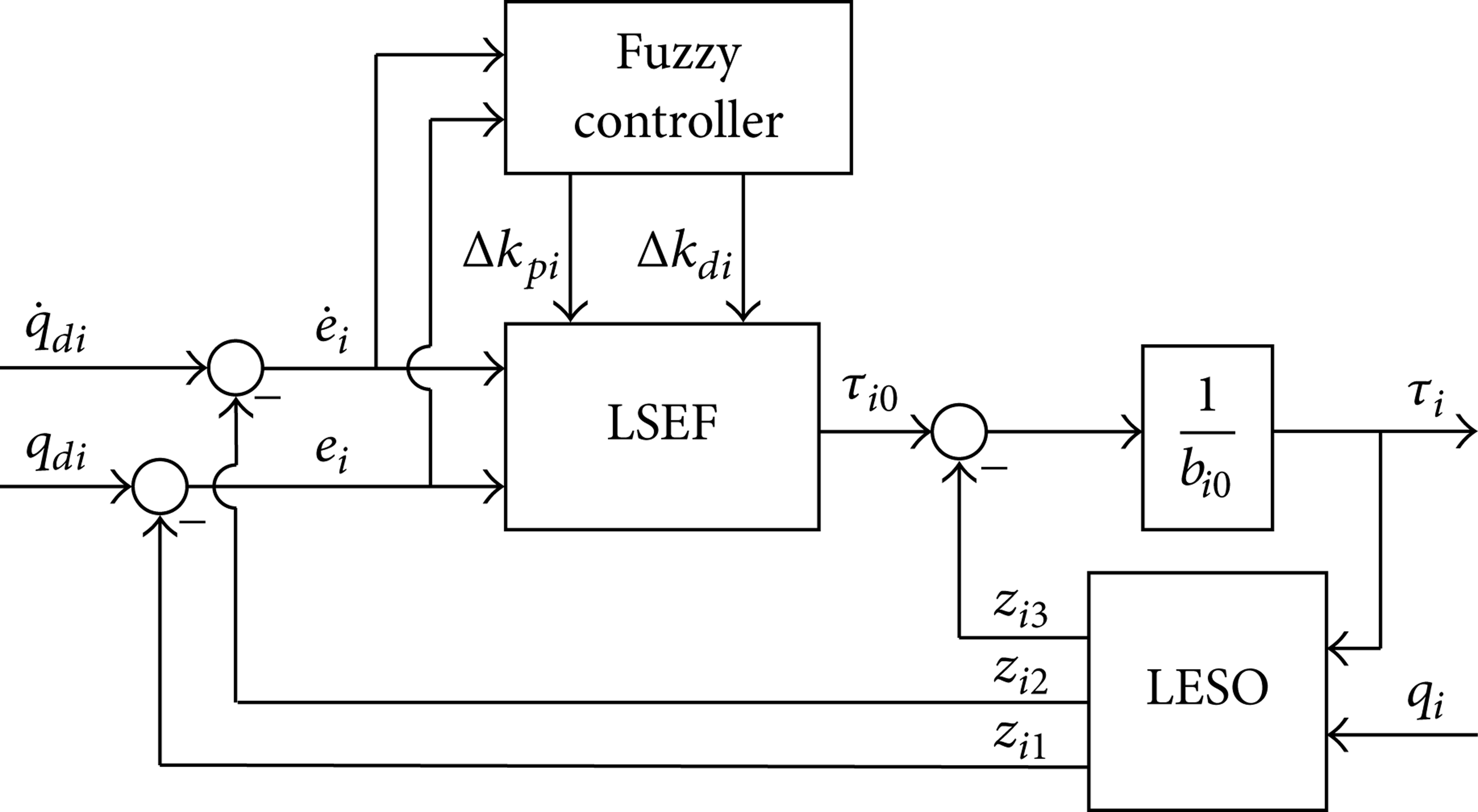
The structure of FSDDC.

As shown in Figure 8, the membership functions are used for the fuzzification of the inputs, which are error e _i and derivative of error ${\dot{e}}_i$ . Here NB, NM, NS, ZO, PS, PM, and PB stand for negative big, negative medium, negative small, zero, positive small, positive medium, and positive big, respectively. The outputs are Δk _pi and Δk _di ; then the initial control gains will be adjusted by the outputs and scale factors as shown in (43). This gives the ability to make the control gain value of the proposed controller smaller or bigger than the gain of the conventional DDC whenever necessary.

Figure 8:

Membership functions: (a) error, (b) derivative of error, (c) gains of Δk _pi , and (d) gains of Δk _di .

The rule tables for Δk _pi and Δk _di are constructed and given in Tables 5 and 6.

Table 5:

Fuzzy rules for Δk _pi .

e i	${\dot{e}}_i$
	NB	NM	NS	ZO	PS	PM	PB
NB	PB	PB	PM	PB	NM	ZO	ZO
NM	PB	PB	PM	PS	PS	ZO	NS
NS	PM	PM	PS	PS	NS	NS	NS
ZO	PM	PM	NS	PB	NS	NM	NM
PS	PS	PS	NS	NS	NS	NM	NM
PM	PS	NM	NS	NM	NM	NM	NB
PB	ZO	ZO	NM	PB	NM	NB	NB

Table 6:

Fuzzy rules for Δk _di .

e i	${\dot{e}}_i$
	NB	NM	NS	ZO	PS	PM	PB
NB	PS	NS	NB	NB	PM	ZO	PS
NM	PS	NS	NB	NM	NM	ZO	ZO
NS	ZO	NS	NM	NM	PS	NS	ZO
ZO	ZO	NS	NS	PB	NS	NS	ZO
PS	ZO	ZO	PS	ZO	ZO	ZO	ZO
PM	PB	NS	PS	PS	PS	PS	PB
PB	PB	PM	PM	NB	PS	PS	PB

Since ξ _i and η _i are chosen to guarantee that the control gains are always kept positive during the fuzzy adaptation, the BIBO stability of the controlled system is preserved.

5. Simulation

A set of numerical simulations is used here to verify the effectiveness of the proposed DDC and FSDDC. In addition, classical PD controller, which is commonly used for control of robot manipulators in industry because of its simple structure, is also applied to the HHA used for comparison. The numerical values of parameters of the HHA are listed in Table 7.

Table 7:

Parameters of the HHA.

Parameters	Values	Unit
l 0	0.5	m
l 1	0.09	m
l 2	0.15	m
l 3	0.09	m
l 4	0.05	m
l 5	0.3	m
l 6	0.103	m
l 10	0.065	m
l 11	0.19	m
l 15	0.28	m
l 30	0.19	m
ρ1	1	kg/m
ρ2	1.5	kg/m
ρ3	2	kg/m
ρ4	1	kg/m
m 9	0.5	kg
g	9.8	m/s2

The reference signals are given in Section 2.2. The initial values of the system are selected as

$\begin{array}{c}{x}_{\mathrm{1}}\left(\mathrm{0}\right)=\mathrm{0.27},\hspace{1em}\hspace{1em}{x}_{\mathrm{2}}\left(\mathrm{0}\right)=\mathrm{0.12},\hspace{1em}\hspace{1em}{x}_{\mathrm{3}}\left(\mathrm{0}\right)=\mathrm{0.15},\\ {\dot{x}}_{\mathrm{1}}\left(\mathrm{0}\right)=\mathrm{0},\hspace{1em}\hspace{1em}{\dot{x}}_{\mathrm{2}}\left(\mathrm{0}\right)=\mathrm{0},\hspace{1em}\hspace{1em}{\dot{x}}_{\mathrm{3}}\left(\mathrm{0}\right)=\mathrm{0}.\end{array}$

(44)

In order to check the robustness of the proposed controllers, a load is introduced and it will be put on the hand in 1.4 seconds to 1.55 seconds; the variation of the mass of the wrist is given in Figure 9.

Figure 9:

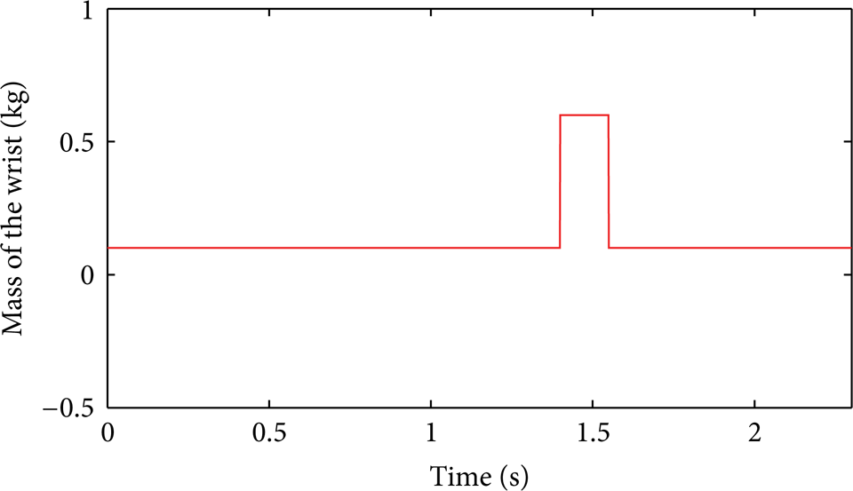
Variation of the mass of the wrist.

Normally, the distributed noise and the parameter uncertainties of the system always exist, which can be thought as disturbing torques acting on the joints, and are assumed to be time varying as

${\tau }_d=\left[\begin{array}{c}\mathrm{20}{\dot{x}}_{\mathrm{1}}+\mathrm{20}\text{sin}\left(x_{\mathrm{1}}\right)+\mathrm{5}\mathrm{sgn}\left({\dot{x}}_{\mathrm{1}}\right)\\ \mathrm{20}{\dot{x}}_{\mathrm{2}}+\mathrm{20}\text{sin}\left(x_{\mathrm{2}}\right)+\mathrm{5}\mathrm{sgn}\left({\dot{x}}_{\mathrm{2}}\right)\\ \mathrm{15}{\dot{x}}_{\mathrm{3}}+\mathrm{15}\text{sin}\left(x_{\mathrm{3}}\right)+\mathrm{3}\mathrm{sgn}\left({\dot{x}}_{\mathrm{3}}\right)\end{array}\right].$

(45)

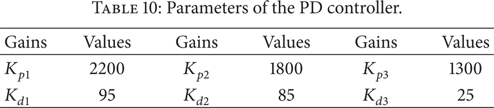
In the following passage, our proposed FSDDC and DDC are used for stabilizing the HHA system in comparison with the PD controller, with the gains of the FSDDC, DDC, and PD controllers being given in Tables 8, 9, and 10.

Table 8:

Parameters of the FSDDC.

Gains	Values	Gains	Values	Gains	Values
b 10	1	b 20	1.3	b 30	1.5
w 01	80	w 02	80	w 03	60
K p1	2200	K p2	2500	K p3	1600
K d1	97	K d2	100	K d3	60
ζ1	400	ζ2	500	ζ3	300
η1	9	η2	10	η3	6

Table 9:

Parameters of the DDC.

Gains	Values	Gains	Values	Gains	Values
b 10	1	b 20	1.3	b 30	1.5
w 01	80	w 02	80	w 03	60
K p1	2200	K p2	2500	K p3	1600
K d1	97	K d2	100	K d3	60

Table 10:

Parameters of the PD controller.

Gains	Values	Gains	Values	Gains	Values
K p1	2200	K p2	1800	K p3	1300
K d1	95	K d2	85	K d3	25

The dynamic tracking performances of the proposed FSDDC are illustrated in Figure 10, and one can find that the proposed FSDDC provides a reasonable tracking capability in the various disturbances and uncertainties. The mass variation applied after 1.4 seconds almost does not affect the tracking performance.

Figure 10:

Responses to desired throwing trajectories under DDC. (a) Position responses of S1, (b) position responses of S2, (c) position responses of S3, (d) velocity responses of S1, (e) velocity responses of S2, and (f) velocity responses of S3.

Figure 11 illustrates the position tracking errors. For a clear comparison, the requested input thrusts of the two controllers are shown in Figure 12.

Figure 11:

Comparison of position tracking errors. (a) Tracking error of S1, (b) tracking error of S2, and (c) tracking error of S3.

Figure 12:

Comparison of input thrust. (a) Input thrust of M1, (b) input thrust of M2, and (c) input thrust of M3.

It is easy to see that the DDC has better tracking performance than the PD controller; the proposed DDC has the smaller tracking error and more convergence to zero than the PD controller; the performance of DDC is further improved by combination with the FLC; the FSDDC has smaller overshoot and shorter setup time than DDC.

The requested input thrust of the proposed FSDDC and DDC is slightly bigger than that of the PD controller, which are all in the range of output thrust of linear motors, and proves the efficiency of the proposed controller.

As a result, we can conclude that the proposed DDC and FSDDC can give a better tracking over the commonly used PD control. In this situation, the HHA can complete the throwing process as requested.

6. Conclusion

This paper addressed the robust trajectory tracking problem for a serial-parallel hybrid humanoid arm (HHA) throwing process in the presence of uncertainties and disturbances. The FSDDC control, with the advantages of both DDC and FLC, has shown a significant improvement over the PID control under the same conditions. The FSDDC can readily decouple the multi-input and multioutput processes by taking the interactions among different parts of the process as disturbances to be estimated and cancelled; it has strong disturbance rejection ability and robustness to uncertainties, which widely exist in throwing processes. The effectiveness of the designed unique dynamic FSDDC strategy was illustrated by simulation examples. We expect that, as we continue to work with the implementation, we may improve the response even further.