Research on Flexible Joint Stiffness Test and Trajectory Planning of Space Manipulator

Abstract

Both Natural Coordinate Formulation describing rigid bodies and Absolute Nodal Coordinate Formulation describing flexible bodies are used to model a flexible manipulator with flexible joint and flexible link. The torsional stiffness of flexible joint is tested using a specialized stiffness test equipment, and then the nonlinear torsional stiffness is determined by fitting the experimental data. A new trajectory planning function called the cosine-based function is proposed to design the joint trajectory, which is smoother than the fifth-polynomial and cycloidal motion functions. Finally, a one-link manipulator with flexible joint and flexible link is used to compare the performance of the three trajectory planning functions. Results show that residual vibration can be remarkably reduced by the proposed cosine-based function, which exhibits a significantly better performance than the fifth-polynomial and cycloidal motion functions.

1. Introduction

A space manipulator undertakes tasks of cabin translocation, transfer, and installation of equipment, as well as serves as an astronaut auxiliary in a station system. It serves an important function in space engineering, with the advantages of lighter structure, lower launching cost, higher operational speed, greater payload-to-manipulator-weight ratio, smaller actuators, lower energy consumption, and better maneuverability. However, the greatest disadvantage of the space manipulator is the vibration problem due to the flexibility of the joint and link. For instance, it took many cumulative hours in order to damp down the residual vibration in the remote manipulator system in a Space Station-assembly Shuttle flight, which occupied 20% to 30% of the total time [1]. The residual vibration significantly reduces the end-point accuracy of the manipulator. Therefore, the best scheme is in which the flexible manipulator completes the required move with minimal residual vibration.

Joint flexibility and link flexibility are basic reasons of manipulator vibration, which cannot be neglected in the dynamic modeling. Spong [2] first modeled the flexible joint as a linear spring, and this modeling technique was adopted by most researchers [3, 4]. However, simple linear spring is not capable of describing the flexible joint precisely. In the dynamic modeling of flexible link, the assumed mode method is typically used by most researchers. Martins et al. [5] and Tso et al. [6] studied a flexible manipulator using the Lagrangian equation and the assumed mode method. In assumed mode model formulation, the link flexibility is usually represented by a truncated finite modal series in terms of spatial mode eigenfunctions and time-varying mode amplitudes. The main drawback of this method is that there are several ways to choose link boundary conditions and mode eigenfunctions. Moreover, the assumed mode method is only capable of describing small deformation, not large deformation. The previous works solely focused on either joint flexibility or link flexibility.

Several different approaches have been suggested to reduce residual vibration, which can be categorized as active control, passive control, and trajectory planning methods. Different trajectories of joint space, significantly affect the vibration of a flexible manipulator. The fifth-polynomial function is widely used to plan the joint trajectory, but it contains the undesirable higher harmonics that excite the system resonances. Cycloidal motion [7] is another trajectory planning function of joint space, whose performance is not clear.

Due to the above deficiencies in the previous work, both Natural Coordinate Formulation (NCF) [8] describing rigid bodies and Absolute Nodal Coordinate Formulation (ANCF) [9, 10] especially suitable for flexible bodies with large deformation are applied to model the flexible manipulator in this paper. The flexibilities of joint and link are simultaneously considered in the dynamic model. The torsional stiffness of flexible joint is tested by a specialized stiffness test equipment, and the nonlinear torsional stiffness is finally determined by fitting the experiment data, which is more precise than the constant torsional stiffness in describing the flexible joint. To suppress the residual vibration, a new planning function called the cosine-based function is proposed to design the joint trajectory. Finally, a one-link manipulator with flexible joint and flexible link is used to verify the effectiveness of the proposed cosine-based function.

This paper is organized as follows. Section 2 is dedicated to the dynamic modeling of a flexible manipulator by NCF and ANCF, with flexible joint and flexible link considered. Section 3 is devoted to the torsional stiffness test for the flexible joint. In Section 4, two trajectory planning functions of the joint are introduced first and then a new planning function called the cosine-based function is proposed. Section 5 gives simulation results and analyses. Finally, the related conclusions are drawn in Section 6.

2. Dynamic Modeling of a Flexible Manipulator

The one-link manipulator with flexible joint and flexible link is shown in Figure 1. The motor rotor and the joint shell are rigid bodies modeled by NCF. They are connected by a torsional spring, whose stiffness is determined from the test experiment introduced in Section 3. The link is a flexible body modeled by ANCF.

Figure 1:

One-link manipulator with flexile joint and flexible link.

NCF is adopted to describe rigid bodies, as shown in Figure 2. The position vectors of two fixed points and two unit vectors on the rigid body are set as generalized coordinates expressed as

$\mathbf{q}={\left[\begin{array}{cccc}{\mathbf{r}}_i^{\text{T}}& {\mathbf{r}}_j^{\text{T}}& {\mathbf{u}}^{\text{T}}& {\mathbf{v}}^{\text{T}}\end{array}\right]}^{\text{T}}.$

(1)

Figure 2:

Space rigid body described by NCF.

The global position vector of an arbitrary point on the rigid body can be written as

$\mathbf{r}=\mathbf{C}\mathbf{q},$

(2)

where C is the element shape function expressed as

$\mathbf{C}=\left[\begin{array}{cccc}\left(\mathrm{1}-c_{\mathrm{1}}\right){\mathbf{I}}_{\mathrm{3}}& c_{\mathrm{1}}{\mathbf{I}}_{\mathrm{3}}& c_{\mathrm{2}}{\mathbf{I}}_{\mathrm{3}}& c_{\mathrm{3}}{\mathbf{I}}_{\mathrm{3}}\end{array}\right],$

(3)

where I₃ is the unit matrix and c₁, c₂, and c₃ are constant components of the local coordinate.

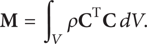
According to the principle of virtual work, the constant mass matrix can be determined as

$\mathbf{M}={\int }_V\rho {\mathbf{C}}^{\text{T}}\mathbf{C}\hspace{0.17em}dV.$

(4)

The three-dimensional beam element of two nodes described by ANCF, as shown in Figure 3, as first proposed by Shabana and Yakoub [9, 10], is used to describe the flexible link. The generalized coordinates of the beam element are written as

$\mathbf{e}={\left[{\mathbf{r}}_i^{\text{T}},{\mathbf{r}}_{i,x}^{\text{T}},{\mathbf{r}}_{i,y}^{\text{T}},{\mathbf{r}}_{i,z}^{\text{T}},{\mathbf{r}}_j^{\text{T}},{\mathbf{r}}_{j,x}^{\text{T}},{\mathbf{r}}_{j,y}^{\text{T}},{\mathbf{r}}_{j,z}^{\text{T}}\right]}^{\text{T}}.$

(5)

Figure 3:

Three-dimensional beam element of two nodes described by ANCF.

The global position vector of an arbitrary point on the body can be written as

$\mathbf{r}=\mathbf{S}\mathbf{e},$

(6)

where S is the element shape function expressed as

$\mathbf{S}=[s_{\mathrm{1}}{\mathbf{I}}_{\mathrm{3}},l{s}_{\mathrm{2}}{\mathbf{I}}_{\mathrm{3}},l{s}_{\mathrm{3}}{\mathbf{I}}_{\mathrm{3}},l{s}_{\mathrm{4}}{\mathbf{I}}_{\mathrm{3}},s_{\mathrm{5}}{\mathbf{I}}_{\mathrm{3}},l{s}_{\mathrm{6}}{\mathbf{I}}_{\mathrm{3}},l{s}_{\mathrm{7}}{\mathbf{I}}_{\mathrm{3}},l{s}_{\mathrm{8}}{\mathbf{I}}_{\mathrm{3}}],$

(7)

where I₃ is the unit matrix. s₁ = 1 – 3ξ² + 2ξ³, s₂ = ξ – 2ξ² + ξ³, s₃ = η – ξη, s₄ = ζ – ξζ, s₅ = 3ξ² – 2ξ³, s₆ = – ξ² + ξ³, s₇ = ξη, s₈ = ξζ; ξ = x/l, η = y/l, and ζ = z/l. x, y, and z are the local coordinates of the element. $x∊\left[\begin{array}{cc}\mathrm{0}& l\end{array}\right]$ , and l is the initial length of the element.

By using the first class of Lagrange's equation, the equations of the motions for constrained rigid-flexible multibody systems can be expressed in a compact form as a set of differential and algebraic equations written as [11]

$\begin{array}{c}\mathbf{M}\stackrel{‥}{\mathbf{q}}+{\mathbf{C}}_{\mathbf{q}}^{\text{T}}\mathbf{\lambda }=\mathbf{Q}\left(\mathbf{q}\right)-\mathbf{F}\left(\mathbf{q}\right),\\ \mathbf{C}\left(\mathbf{q},t\right)=\mathbf{0},\end{array}$

(8)

where M is the mass matrix, q denotes the generalized coordinates, C stands for the constraint equations, C _q is the Jacobi of constraint equations, λ is the Lagrangian multiplier, Q is the generalized external force, and F is the generalized elastic force. The calculation of the elastic force and its Jacobi can be referred to in [12, 13].

Several algorithms can be used to solve differential-algebraic equations of multibody system numerically. These algorithms include the Baumgarte, Newmark, generalized-a, and augmented Lagrangian methods. In this paper, the iteration strategy of the generalized-a method proposed by Arnold and Br $\stackrel{‥}{\text{u}}$ ls [14] and the scaling technology proposed by Bottasso et al. [15] are adopted for numerically solving the differential-algebraic equations efficiently and precisely.

3. Torsional Stiffness Test for the Flexible Joint

The specialized stiffness test equipment developed by our research group is used to test the torsional stiffness of the flexible joint. The optical schematic of double angle is shown in Figure 4. The laser beam emitted by the laser locates at point A₀ on the screen after being reflected by the mirror. According to the basic optical principle, if the mirror rotates by α degree, the reflected laser beam rotates by 2α degree, and the laser spot on the screen moves from point A₀ to point A₁. Let the moving distance of the laser spot be Δ _A , and let the distance from the mirror to the screen be S _A . S _A is generally significantly greater than Δ _A ; that is, S _A ≫ Δ _A . Thus, α has a small value. According to the triangle geometry, the rotation angle of the mirror can be obtained as

$\alpha =\frac{{\mathrm{\Delta }}_A}{\mathrm{2}{S}_A}.$

(9)

Figure 4:

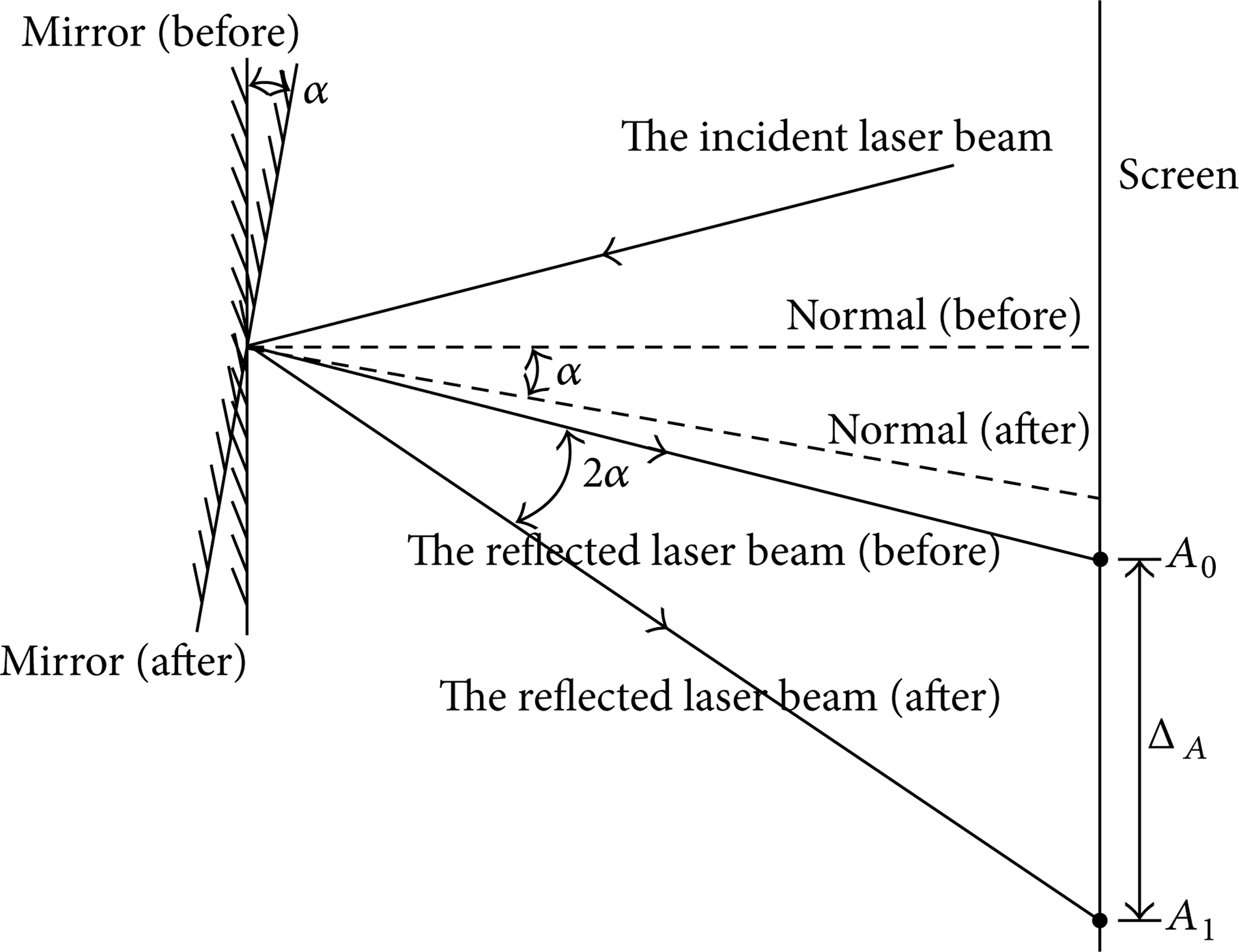
Optical schematic of double angle.

The stiffness test schematic is shown in Figure 5. Let A be the measuring point and let B be the reference point. Two mirrors are attached to points A and B separately. The two lasers emit laser beams, and the laser beams, respectively, locate at points A₀ and B₀ on the screen after being reflected by the mirrors. When torque τ is applied to the joint, the two mirrors rotate by α _A and α _B . According to the basic optical principle, the reflected laser beams rotate by 2α _A and 2α _B , and the laser spots on the screen move from points A₀ and B₀ to points A₁ and B₁, respectively. The moving distances of laser spots are Δ _A and Δ _B . Then, the rotational angle of the measuring point A relative to the rotational angle of the datum point B can be obtained as

$\alpha ={\alpha }_A-{\alpha }_B=\frac{{\mathrm{\Delta }}_A}{\mathrm{2}{S}_A}-\frac{{\mathrm{\Delta }}_B}{\mathrm{2}{S}_B}.$

(10)

Figure 5:

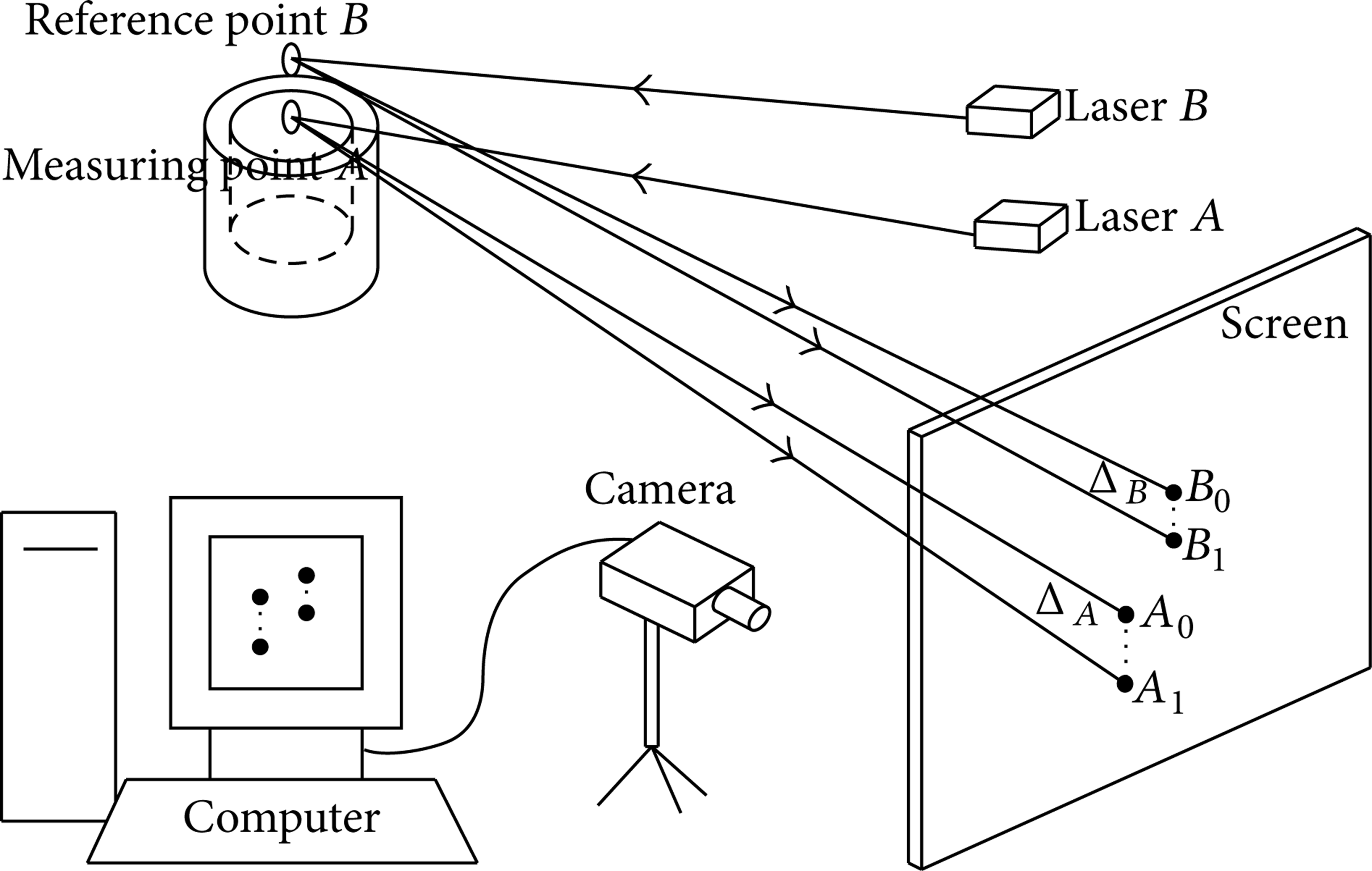
Schematic of torsional stiffness test.

A mechanical testing machine is used to apply torque τ _i to the joint, after which the relative angle α _i is measured. The typical τ-α curve is shown in Figure 6.

Figure 6:

Torque-angle curve.

The torque-angle curve has two segments: nonlinear and linear. The quadratic polynomial is adopted to fit the nonlinear segment, whereas the least square method is adopted to fit the linear segment. Finally, the relationship between torque and angle can be expressed by the following formula:

$\tau =\{\begin{array}{cc}{\tau }_{\mathrm{1}}{\left(\frac{\alpha }{{\alpha }_{\mathrm{1}}}\right)}^{\mathrm{2}},\hfill & \left|\alpha \right|<{\alpha }_{\mathrm{1}},\hfill \\ {\tau }_{\mathrm{1}}+K_{\mathrm{1}}\left(\alpha -{\alpha }_{\mathrm{1}}\right),\hfill & \left|\alpha \right|\ge {\alpha }_{\mathrm{1}},\hfill \end{array}$

(11)

where (α₁, τ₁) is the turning point between nonlinear segment and linear segment and K₁ is the stiffness of linear segment.

The nonlinear stiffness of the joint, as shown in Figure 7, can be obtained by differentiating the above equation.

Figure 7:

Nonlinear stiffness of the joint.

4. Trajectory Planning of the Joint

In engineering, smooth and continuous functions are typically adopted to plan the joint trajectory, the first and second derivatives of which are also smooth and continuous, such as the fifth-polynomial and cycloidal motion functions. The six boundary conditions of angle, angular velocity, and angular acceleration of the joint are as follows:

$\begin{array}{c}\stackrel{\sim }{\theta }\left(\mathrm{0}\right)={\theta }_{\mathrm{0}},\hspace{1em}\hspace{1em}\dot{\stackrel{\sim }{\theta }}\left(\mathrm{0}\right)=\mathrm{0},\hspace{1em}\hspace{1em}\stackrel{‥}{\stackrel{\sim }{\theta }}\left(\mathrm{0}\right)=\mathrm{0},\\ \stackrel{\sim }{\theta }\left(t_f\right)={\theta }_f,\hspace{1em}\hspace{1em}\dot{\stackrel{\sim }{\theta }}\left(t_f\right)=\mathrm{0},\hspace{1em}\hspace{1em}\stackrel{‥}{\stackrel{\sim }{\theta }}\left(t_f\right)=\mathrm{0},\end{array}$

(12)

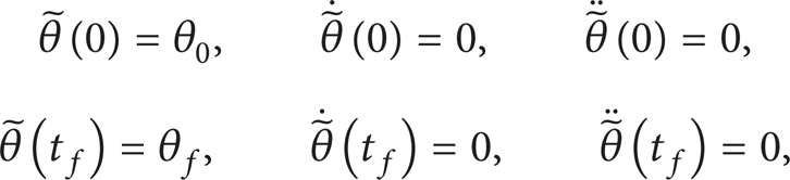
where t _f is the planning time, θ₀ is the initial angle of joint, and θ _f is the final angle of joint.

(1) The fifth-polynomial is adopted to plan the joint trajectory. The polynomial coefficients are obtained by the six boundary conditions described by (12). Finally, the angle, angular velocity, and angular acceleration of the joint are as follows:

$\begin{array}{c}\stackrel{\sim }{\theta }=\left({\theta }_f-{\theta }_{\mathrm{0}}\right)\left[\mathrm{6}{\left(\frac{t}{t_f}\right)}^{\mathrm{5}}-\mathrm{15}{\left(\frac{t}{t_f}\right)}^{\mathrm{4}}+\mathrm{10}{\left(\frac{t}{t_f}\right)}^{\mathrm{3}}\right]+{\theta }_{\mathrm{0}},\\ \dot{\stackrel{\sim }{\theta }}=\frac{\left({\theta }_f-{\theta }_{\mathrm{0}}\right)}{t_f}\left[\mathrm{30}{\left(\frac{t}{t_f}\right)}^{\mathrm{4}}-\mathrm{60}{\left(\frac{t}{t_f}\right)}^{\mathrm{3}}+\mathrm{30}{\left(\frac{t}{t_f}\right)}^{\mathrm{2}}\right],\\ \stackrel{‥}{\stackrel{\sim }{\theta }}=\frac{\left({\theta }_f-{\theta }_{\mathrm{0}}\right)}{t_f^{\mathrm{2}}}\left[\mathrm{120}{\left(\frac{t}{t_f}\right)}^{\mathrm{3}}-\mathrm{180}{\left(\frac{t}{t_f}\right)}^{\mathrm{2}}+\mathrm{60}\left(\frac{t}{t_f}\right)\right].\end{array}$

(13)

(2) Cycloidal motion is adopted to plan the joint trajectory expressed as

$\stackrel{\sim }{\theta }\left(t\right)=\left({\theta }_f-{\theta }_{\mathrm{0}}\right)\left[\frac{t}{t_f}-\frac{\mathrm{1}}{\mathrm{2}\pi }\text{sin}\left(\frac{\mathrm{2}\pi t}{t_f}\right)\right]+{\theta }_{\mathrm{0}}.$

(14)

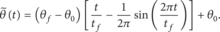
The angular velocity and angular acceleration of the joint can be obtained by differentiating the above equation and can be determined as

$\begin{array}{c}\dot{\stackrel{\sim }{\theta }}\left(t\right)=\frac{\left({\theta }_f-{\theta }_{\mathrm{0}}\right)}{t_f}\left[\mathrm{1}-\text{cos}\left(\frac{\mathrm{2}\pi t}{t_f}\right)\right],\\ \stackrel{‥}{\stackrel{\sim }{\theta }}\left(t\right)=\frac{\left({\theta }_f-{\theta }_{\mathrm{0}}\right)}{t_f^{\mathrm{2}}}\left[\mathrm{2}\pi \text{sin}\left(\frac{\mathrm{2}\pi t}{t_f}\right)\right].\end{array}$

(15)

Cycloidal motion can evidently satisfy all boundary conditions described by (12).

(3) In this paper, a cosine-based function is proposed to plan the joint trajectory, and it can be written as

$\stackrel{\sim }{\theta }\left(t\right)=\left({\theta }_f-{\theta }_{\mathrm{0}}\right)\left[a_{\mathrm{0}}+a_{\mathrm{1}}\text{cos}\left(\frac{\pi t}{t_f}\right)+a_{\mathrm{3}}\text{cos}\left(\frac{\mathrm{3}\pi t}{t_f}\right)\right]+{\theta }_{\mathrm{0}}.$

(16)

According to the six boundary conditions described by (12), the three unknown coefficients a₀, a₁, and a₃ can be determined. Finally, the angle, angular velocity, and angular acceleration of the joint are as follows:

$\begin{array}{c}\stackrel{\sim }{\theta }\left(t\right)=\left({\theta }_f-{\theta }_{\mathrm{0}}\right)\left[\frac{\mathrm{1}}{\mathrm{2}}-\frac{\mathrm{9}}{\mathrm{16}}\text{cos}\left(\frac{\pi t}{t_f}\right)+\frac{\mathrm{1}}{\mathrm{16}}\text{cos}\left(\frac{\mathrm{3}\pi t}{t_f}\right)\right]+{\theta }_{\mathrm{0}},\\ \dot{\stackrel{\sim }{\theta }}\left(t\right)=\frac{\left({\theta }_f-{\theta }_{\mathrm{0}}\right)}{t_f}\left[\frac{\mathrm{9}}{\mathrm{16}}\pi \text{sin}\left(\frac{\pi t}{t_f}\right)-\frac{\mathrm{3}}{\mathrm{16}}\pi \text{sin}\left(\frac{\mathrm{3}\pi t}{t_f}\right)\right],\\ \stackrel{‥}{\stackrel{\sim }{\theta }}\left(t\right)=\frac{\left({\theta }_f-{\theta }_{\mathrm{0}}\right)}{t_f^{\mathrm{2}}}\left[\frac{\mathrm{9}}{\mathrm{16}}{\pi }^{\mathrm{2}}\text{cos}\left(\frac{\pi t}{t_f}\right)-\frac{\mathrm{9}}{\mathrm{16}}{\pi }^{\mathrm{2}}\text{cos}\left(\frac{\mathrm{3}\pi t}{t_f}\right)\right].\end{array}$

(17)

The maximal angular velocity and angular acceleration of the fifth-polynomial, cycloidal motion, and cosine-based functions are shown in Table 1. The ratio of the maximal angular velocity of the three functions is 1: 1.07: 1.26, and the ratio of the maximal angular acceleration of the three functions is 1: 1.09: 1.48.

Table 1:

Maximal angular velocity and angular acceleration of the three planning functions.

	Fifth-polynomial function	Cycloidal motion function	Cosine-based function
${\dot{\stackrel{\sim }{\theta }}}_{\max }$	$\frac{\mathrm{15}}{\mathrm{8}}\left(\frac{{\theta }_f-{\theta }_{\mathrm{0}}}{t_f}\right)$	$\mathrm{2}\left(\frac{{\theta }_f-{\theta }_{\mathrm{0}}}{t_f}\right)$	$\frac{\mathrm{3}}{\mathrm{4}}\pi \left(\frac{{\theta }_f-{\theta }_{\mathrm{0}}}{t_f}\right)$
${\stackrel{‥}{\stackrel{\sim }{\theta }}}_{\max }$	$\frac{\mathrm{10}}{\sqrt{\mathrm{3}}}\left(\frac{{\theta }_f-{\theta }_{\mathrm{0}}}{t_f^{\mathrm{2}}}\right)$	$\mathrm{2}\pi \left(\frac{{\theta }_f-{\theta }_{\mathrm{0}}}{t_f^{\mathrm{2}}}\right)$	$\frac{\sqrt{\mathrm{3}}}{\mathrm{2}}{\pi }^{\mathrm{2}}\left(\frac{{\theta }_f-{\theta }_{\mathrm{0}}}{t_f^{\mathrm{2}}}\right)$

The planning time t _f is set to be 1 [s], the initial angle θ₀ is set to be 0°, and the final angle θ _f is set to be 5°.

Figures 8, 9, and 10 show the angle, angular velocity, and angular acceleration of the three planning functions, respectively. The angle, angular velocity, and angular acceleration of the cosine-based function are smoother than those of the fifth-polynomial and cycloidal motion functions at the initial and final times, whereas the maximal angular velocity and the maximal angular acceleration of the cosine-based function are larger than those of the fifth-polynomial and cycloidal motion functions.

Figure 8:

Joint angle of the three planning functions.

Figure 9:

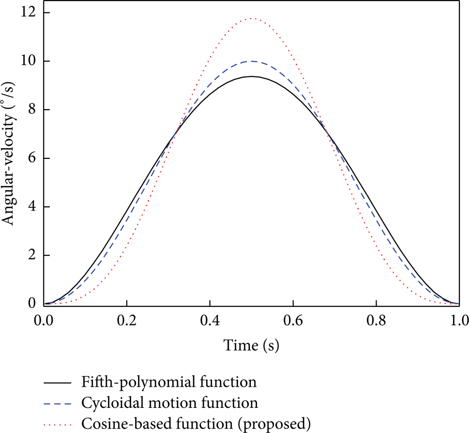
Joint angular velocity of the three planning functions.

Figure 10:

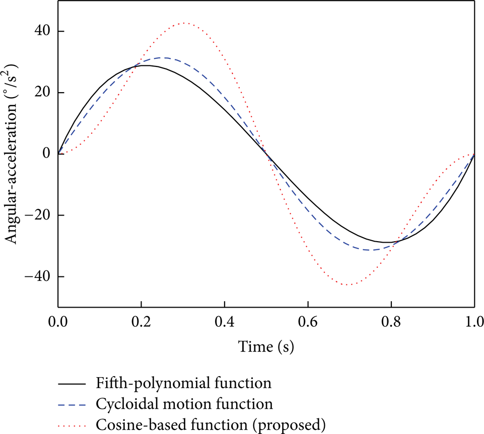
Joint angular acceleration of the three planning functions.

5. Simulation Studies

The planning time is set to be 1 [s], the simulation time is set to be 2 [s], the initial angle of the joint is set to be 0°, and the final angle of the joint is set to be 5°.

The geometrical parameters and mechanical parameters of the flexible link are shown in Table 2. Also, six ANCF three-dimensional beam elements are used to discretized the flexible link.

Table 2:

Parameters of the flexible manipulator link.

Length	Inner radius	Outer radius	Young's modulus	Poisson's ratio
3.5 (m)	6 (cm)	8 (cm)	90 (GPa)	0.3

The above three planning functions are used to plan the joint trajectory. The motor is driven by the speed mode; that is, the motor rotor is assumed to be capable of absolutely tracking the given trajectory using the three planning functions, respectively. To determine the effects of the three planning functions on manipulator vibration, two cases are studied: (1) with joint flexibility considered and (2) with joint flexibility and link flexibility considered.

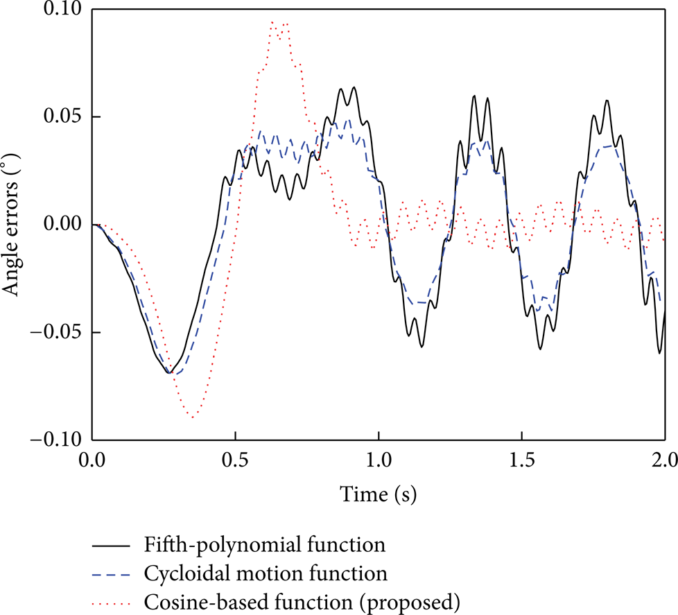
Figure 11 shows the angle errors of the three planning functions with joint flexibility considered. In the course of motion (0 s ≤ t ≤ 1 s), the maximal angle errors of the fifth-polynomial, cycloidal motion, and cosine-based functions are, respectively, 0.056°, 0.052°, and 0.056°, whereas after motion (1 s ≤ t ≤ 2 s), the residual angle errors are, respectively, 0.028°, 0.019°, and 0.002°. The tracking errors caused by the three functions are evidently similar in the course of motion, but the residual vibration caused by the proposed cosine-based function is far less than that caused by the fifth-polynomial and cycloidal motion functions after motion.

Figure 11:

Angle errors of the joint (with joint flexibility considered).

Figure 12 shows the angle errors of the joint of the three planning functions with joint flexibility and link flexibility considered. Figure 13 shows the vibration of the endpoint of the three planning functions with joint flexibility and link flexibility considered. In the course of motion (0 s ≤ t ≤ 1 s), the maximal angle errors of the fifth-polynomial, cycloidal motion, and cosine-based functions are, respectively, 0.069°, 0.070°, and 0.095°, whereas the maximal vibration amplitudes of the endpoint are, respectively, 1.84 cm, 1.87 cm, and 2.38 cm. After motion (1 s ≤ t ≤ 2 s), the maximal residual angle errors are, respectively, 0.060°, 0.040°, and 0.012°, whereas the maximal residual vibration amplitudes of the endpoint are, respectively, 1.43 cm, 1.03 cm, and 0.10 cm. The tracking errors caused by the three functions are evidently similar in the course of motion, but the error caused by the cosine-based function is a lightly higher. However, the residual vibration caused by the cosine-based function is significantly less than that caused by the fifth-polynomial and cycloidal motion functions after motion.

Figure 12:

Angle errors of the joint (with joint flexibility and link flexibility considered).

Figure 13:

Vibration of the endpoint (with joint flexibility and link flexibility considered).

The above analysis shows that, whether with joint flexibility considered or with both joint flexibility and link flexibility considered, the tracking errors caused by the three planning functions are similar in the course of motion, but the residual vibration caused by the cosine-based function proposed in this paper is significantly less than that caused by the fifth-polynomial and cycloidal motion functions after motion. We can thus conclude that the cosine-based planning function proposed in this paper is more effective in weakening the residual vibration than the fifth-polynomial planning and cycloidal motion planning functions.

6. Conclusions

The flexible manipulator is modeled by NCF and ANCF, considering the flexibility of joint and link. The nonlinear torsional stiffness is finally determined by fitting the experimental data. Moreover, a cosine-based function is proposed to suppress the residual vibration. The maximal angular velocity ratio and angular acceleration ratio of the fifth-polynomial, cycloidal motion, and cosine-based functions are, respectively, 1: 1.07: 1.26 and 1: 1.09: 1.48. A one-link manipulator with flexible joint and flexible link is used to evaluate the proposed trajectory planning function. Results show that the residual vibration by the proposed cosine-based function is reduced to 7.1% of that by the fifth-polynomial function and to 9.7% of that by the cycloidal motion function.

Notably, the effectiveness of the proposed cosine-based function in weakening the residual vibration is only verified by numerical simulations. The corresponding experimental validation is left for our future work.