Sage Journals: Discover world-class research

Abstract

This paper compares and analyzes the quantitative diagnosis methods based on Lempel-Ziv complexity for bearing fault, using continuous wavelet transform (CWT), Empirical Mode Decomposition (EMD) method, and wavelet packet method for decomposition of vibration signal measured by acceleration sensors, respectively. The kurtosis and entropy indices are also analyzed in order to select the optimum analysis area from the vibration signal. The variation trend of vibration signal Lempel-Ziv complexity of bearing inner race and outer race with the varying fault severity is analyzed and predicted based on the generation mechanism and characteristics of fault vibration signals. Experimental results show that it is suitable for observing the fault growing trend and severity by examining the value based on improved Lempel-Ziv complexity algorithm using continuous wavelet transform (CWT), Empirical Mode Decomposition (EMD) method, and wavelet packet method for signal decomposition, using kurtosis indices for optimal analysis area selection, and using the optimal weight coefficients for complexity calculation.

1. Introduction

The rolling bearing is one of the most widely used general mechanical components in rotating machines. Its running state directly affects the performance of the whole machine, and the fault degree quantitative identification and diagnosis can prolong the service life and reduce the production cost. Therefore, the rolling bearing's condition monitor especially quantitative fault diagnosis has very important practical significance.

The state of bearing is usually analyzed by vibration signal which is acquired by acceleration sensor. However, rolling bearing fault is a dynamic development process, and rolling bearing early weak fault vibration signal is so complex, often mixed with large amount of background noise, that the rolling bearing quantitative diagnosis gets more difficult.

Aiming at solving this problem, domestic and foreign scholars have made much more beneficial attempts. For example, Zhang et al.[1] concerned with the application of fuzzy neural networks which made use of information from both the fault symptoms and the fault patterns to realize the fault degree diagnosis for rotary machines. Dong and Chen [2] proposed the cycle frequency energy index to quantitative characterization of the rolling bearing damage based on the second order steady theory and bearing vibration signal cycle coherence analysis. Feng et al. [3] introduced degradation indicators to proportional failure rate model and achieved effective assessment of equipment operation in the vibration signal of different degrees of injury. Pan et al. [4] extracted feature vectors with lifting wavelet packet decomposition and built assessment model utilizing fuzzy c-means to achieve the distinction of bearing normal circumstances, slight fault, and serious faultLindh et al. [5] trained the signal and then diagnosed the bearing fault qualitatively from the classification result using the methods of multivariate statistical fault classification and fuzzy logic.

Some scholars used the theory of complexity to identify the degree of bearing failure proposed by Lempel and Zip. They made those fuzzy concepts “simple” “complex” qualitative by this theory and conducted quantitative fault diagnosis of bearing. For example, the continuous wavelet transform signal decomposition method combined with the complexity theory is used to identify the fault degree [6, 7]. EMD is used to decompose signal and calculate the Lempel-Ziv complexity value in the optimum analysis area [8 –10]. In summary, it is feasible to identify the fault degree of the bearing by using the complexity theory. However, there are some differences in the complexity calculation process and results due to different signal processing.

Complexity algorithm for bearing fault quantitative diagnosis can be divided into the following five steps:

apply time-frequency analysis method to decompose vibration signal;

obtaining the optimum analysis area from the decomposed signal in step 1;

calculate high- and low-frequency complexity values of the decomposed signal at the optimum analysis area;

calculate the ultimate Lempel-Ziv complexity value by using the weight coefficients of high and low frequencies of bearing's inner and outer rings;

diagnose the rolling bearing fault degree according to the complexity value variation trend.

The process is shown in Figure 1.

Figure 1:

The calculation process of Lempel-Ziv complexity.

It is clear that in step 1, the practical way of time-frequency analysis method is not unique [6 –9], therefore, in which time-frequency analysis method is effective or better need to be further studied.

In step 2, the predecessors have chosen the kurtosis index [8 –10] to get the best scale level. We can try to use other different indexes for better results.

Finally, predecessor's research is lack of basis in step 4 (the selection of weight coefficients). It is worth to do some research work on the optimization of the coefficient.

This paper analyzes generation mechanism of fault vibration signals of bearing and the cause of change in complexity value combining with the physical meaning of Lempel-Ziv complexity, and then a comparative study is researched in three different frequency analysis methods of the continuous wavelet transform (CWT), EMD and the wavelet packet decomposition combining with two indices of the kurtosis and entropy. Finally, the scope of the weight coefficients is given under the analysis of bearing fault mechanism. Experimental results show that it is suitable for observing the fault growing trend and severity by examining the value based on improved Lempel-Ziv complexity algorithm using continuous wavelet transform (CWT), Empirical Mode Decomposition (EMD) method, and wavelet packet method for signal decomposition, using kurtosis indices for optimal analysis area selection, and using the optimal weight coefficients for complexity calculation.

2. Lempel-Ziv Complexity Theory

Ziv and Lempel introduced an easily calculable measurement of complexity of finite sequences [11, 12]. Consider a string X(n), firstly making binary conversion to X(n)—that is, if $(i) \geq mean (X (n))$ (i = 1, 2, 3, … n), define S(i) = 1 (i = 1, 2, 3, … n); if not, S(i) = 0, getting S(n) = {s₁, s₂, … s_n}—the Lempel-Ziv index of S(n) can be calculated through the cycle.

Lempel-Ziv complexity algorithm can be divided into the following five steps:

when r = 0, define S_{v, 0} = {}, Q₀ = {}, and C_n(0) = 0. When r = 1, take $Q_{1} = {Q_{0} s_{1}},$ as Q₁ does not belong to S_{v, 0}; therefore, C_n(1) = C_n(0) + 1 = 1, Q₁ = {}, and r = r + 1;

take Q_r = {Q_{r – 1}s_r} and S_{v, r – 1} = {S_{v, r – 2}s_{r – 1}}; ask if Q_r belongs to the vocabulary of S_{v, r – 1}. If so, string C_n(r) = C_n(r – 1) and r = r + 1. If not, C_n(r) = C_n(r) + 1, Q_r = {}, and r = r + 1; repeat step 2; loop n times.

C_n(r) is obviously affected by the length of S(n). To get relatively independent indicators, Lempel and Ziv further proposed the following normalized formula:

\begin{matrix} 0 \leq C_{n} = \frac{C_{n} (n)}{C_{u l, n}} \leq 1, \\ C_{u l, n} = \lim_{n \to \infty} C_{n} (n) = \frac{n}{lo g_{2} n} . \end{matrix}

(1)

Calculate Lempel-Ziv complexity through this normalized formula.

The calculation method of Lempel-Ziv complexity can be explained as the closeness of the signal time series and random sequence or the quantity of frequency components. The C_{ul, n} of completely random sequence tends to be 1, while the C_{ul, n} of periodic sequence tends to be 0. When C_{ul, n} ∊ (0, 1), the sequence between the two cases above.

The greater the complexity of the sequence, the less the periodic component in the sequence, and the more irregular and random state the sequence will be, which means the signal sequence contains more frequency components. The smaller the complexity of the sequence, the more the periodic components in the sequence, and the more regular and periodic state the sequence will be in, which means the sequence contains less frequency components.

The complexity of the algorithm is a relative concept [13] taking into account the practical significance of the complexity of the algorithm. It is possible to reflect the features of signal only if it is representative. Therefore, analysis area of complexity must fully reflect the true shape of signal.

3. Signal Time-Frequency Analysis Methods

The analysis areas must be decomposed and extracted from the vibration sequence of fault bearing before using complex algorithms to analyze. The quality of analysis area is very important to the results. Therefore, determining the analysis area of complex is the key point in the fault degree diagnosis of rolling bearing.

This paper is focused on these three time-frequency analysis methods used frequently to get the decomposed analysis area of continuous wavelet transform (CWT), EMD method, and wavelet packet method.

3.1. Continuous Wavelet Transform Complexity Theory

Wavelet analysis [14] is one of the most common methods of signal analysis. Take ψ(t) as a square integrable function; that is ψ(t) ∊ L²(R), if Fourier transformation $\hat{ψ} (ω)$ meets the admissibility conditions:

C_{ψ} = \int_{- \infty}^{+ \infty} \frac{{| \hat{ψ} (ω) |}^{2}}{| ω |} d ω < \infty,

(2)

where ψ(t) is called mother function.

Variables a and b are defined as dilation factor and displacement factor; the dilation factor a indicates the wavelet's width, and the displacement factor b gives its position to generate ψ_{a, b}(t):

ψ_{a, b} (t) = {| a |}^{- 1 / 2} ψ (\frac{t - b}{a}),

(3)

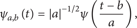
where ψ_{a, b}(t) is the wavelet basis function depending on factors a and b, also known as continuous wavelet basis function.

When continuous-time signal x(t) ∊ L²(R), continuous wavelet transform is defined as

W_{b} (a) = 〈 ψ_{a, b} (t), x (t) 〉 = {| a |}^{- 1 / 2} \int x (t) ψ_{a, b}^{*} d t .

(4)

To discrete time series x_m, take t = mδt, b = nδt (m, n = 0, 1, 2, …, N are sampling points, and δt is sampling interval); therefore, the continuous wavelet transformation of x_m is

W_{n} (a_{j}) = \sum_{m = 0}^{N - 1} x_{m} ψ^{*} [\frac{(m - n) δ t}{a_{j}}] .

(5)

The coefficient matrix of continuous wavelet transform can be obtained by changing the time indexes j and n corresponding to the dilation factor a and displacement factor b. The coefficient matrix reflects the variation of continuous wavelet transform coefficient's amplitude with the variation of time and scale.

3.2. EMD Theory

EMD [15, 16] supposes every signal consisting of different intrinsic mode function (IMF) and each IMF can be linear or nonlinear. IMF expresses signal's vibration form of the intrinsic characteristics. IMF has to satisfy the following two conditions: (1) extreme point number and the number of zeros are at most a difference of one; (2) the upper and lower envelopes are local symmetry on the timeline.

The nature of EMD method is getting signal intrinsic vibration modes by characteristic time scales and then choosing the intrinsic vibration modes from the signal. EMD decomposition can be divided into two steps.

(1) Identify all extreme points of x(t), getting upper and lower envelopes, and compute the average m₁. Then, extract the detailed m₁ from x(t), filtering out low-frequency trend data and getting the new series h₁, that is,

h_{1} = x (t) - m_{1} .

(6)

Commonly, h₁ unnecessarily meets the IMF's conditions; the above process needs repeating. If the average envelope of h₁ is m₁₁, the low-frequency trend data h₁₁ will have to be filtered out from h₁, that is,

h_{11} = h_{1} - m_{11} .

(7)

The process continues until meeting the filter stop condition and getting the first IMF c₁, which represents the highest frequency component in the local moment.

(2) Extract c₁ from x(t), and get data sequence r₁ that is removed the high-frequency components, getting the second IMF c₂ and repeating this step until r_n becomes monotonic function or the magnitude is very small; step 2 can be stated as

\begin{matrix} r_{1} = x (t) - c_{1}, \\ r_{2} = r_{1} - c_{2}, \\ r_{n} = r_{n - 1} - c_{n} . \end{matrix}

(8)

From (8)

x (t) = \sum_{i = 1}^{n} c_{i} + r_{n} .

(9)

The signal x(t) can be expressed as the sum of several IMF c_i and residual r_n.

3.3. Wavelet Packet Theory

Wavelet analysis [14] has a wide range of applications in signal processing because of its multiresolution in time frequency. However, due to its scale changes according to the binary system, the frequency resolution is high in the low frequency and low in the high-frequency, and the time frequency is low in the low frequency and high in the high frequency.

Wavelet packet analysis has the ability to decompose signal further in the high-frequency part, providing a more sophisticated method of frequency division for signal.

Take ϕ(t) as the orthogonal scaling function and ψ(t) as the wavelet function. For wavelet transform, they satisfy

\begin{matrix} ϕ (t) = \sum_{k} h_{k} ϕ (2 t - k), \\ ψ (t) = \sum_{k} g_{k} ψ (2 t - k) . \end{matrix}

(10)

To further promote the two-scale equation, follow the recursive relationship:

\begin{matrix} ϕ_{2 n} (t) = \sum_{k} h_{k} ϕ_{n} (2 t - k), \\ ϕ_{2 n + 1} (t) = \sum_{k} g_{k} ϕ_{n} (2 t - k) . \end{matrix}

(11)

Define function series {ϕ_n(t)}, n ∊ Z; it is called orthogonal wavelet packet determined by ϕ₀ = ϕ(t), and h_k and g_k are filter coefficients. Wavelet transform is applied h_k, g_k to each filter output. while it is different from multi-resolution of dyadic wavelet, that is not only dividing in low-frequency part of the space, but also dividing in the high-frequency part in a similar way, to bring about the decomposition for an arbitrary tree structure in function space.

Through theoretical analysis showed above, EMD method and wavelet packet method have better adaptability and ability to reflect the signal characteristics, while, which algorithm is effective combining with Lempel-Ziv complexity algorithm in quantitative fault diagnosis of bearing needs to be discussed and analyzed by further experimental data analysis.

4. Selection of Optimal Area for Analysis

After the effective area is divided, the selection of optimal area is required. Optimum analysis area could be defined as the extraction of signal analysis region containing more effective component (fault degree information). On the one hand, the rolling bearing early weak fault vibration signal is very complex, often mixed with large amount of useless signals for fault quantitative diagnosis; it is unwise to calculate complexity with those interference factors. On the other hand, the calculation speed could be improved and the calculation effect could be enhanced, if the computational region could be restricted to the small area containing more useful information (fault degree information).

Thus, the selection of optimal area is required by using some characteristic value after the effective area is divided. The characteristic value selected should be able to reflect the complexity degree of the signals since the complexity refers to signal complexity. Therefore, the commonly used indices are entropy and kurtosis [7 –10, 17 –19].

As an information measure of process under certain state, entropy represents the uncertainty degree of the signal and is often used in fault feature extraction.

Entropy [20] can be defined as

H = - \sum_{i = 1}^{n} p_{i} \log p_{i},

(12)

where p_i is the proportion of certain component of the signal.

The more complex the signal is, the more evenly distributed is the vibration energy in entire frequency components, and the greater the uncertainty degree and the entropy will be. Therefore, entropy can reflect dynamically the changes in the state of rolling bearing and fault severity.

As a normalized time-domain statistic, kurtosis [21] is very sensitive to the transient characteristics of the signal and is widely used in fault diagnosis of machinery and equipment. Kurtosis can be defined as:

ks = \frac{mean ({| x |}^{4})}{{[mean ({| x |}^{2})]}^{2}} - 2 .

(13)

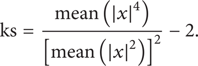
The vibration signals of normal bearing approximately obey normal distribution, and its kurtosis value is about three. Kurtosis will become larger when faults occur. Therefore, for different time intervals of the same vibration sequence, when the kurtosis of some time intervals is more than three, the randomness of these time intervals is less than the random signal and fault can be diagnosed. Larger kurtosis means that this time interval contains more fault information.

By the definition of kurtosis given above, the time intervals with larger kurtosis of rolling bearing signals contain more fault feature information.

In this paper continuous wavelet transform, EMD, and wavelet packet transform can decompose the original signals into some section, which is a one-dimensional vector. Selecting the region with the greatest entropy or kurtosis value is to compute Lempel-Ziv value of the region containing the largest amount of fault degree information which could improve the calculation effect.

5. Complexity Theory of Bearing

When the surface of a bearing component has some local damage, it will collide with the surface of other components that interact with it in the loading process [22]. The periodic impulsive force known as fault feature signal can be measured when using an acceleration sensor to detect the vibration signal in the operation process of fault bearing. Since the frequency band of each impulsive force is quite wide, it inevitably contains the natural frequency of bearing and sensors, thereby stimulating the high-frequency natural vibration of the whole vibration detection system. High-frequency natural vibration model can be regard as a quality-spring-damping system, whose frequency is only associated with the properties of rolling bearing itself. The fault bearing information is usually acquired during bearing running station, and the fault position changes in relation to that of the sensor. This phenomenon will cause the signal amplitude detected by the sensor to vary with fault position, and a low-frequency envelope known as low-frequency modulated signal resulting from non-homogeneous load distribution is generated. Definitely, some noise signals are also contained in the signals detected. However, these signals are mostly high-frequency signals, with great interference of the fault signal analysis.

Bearing fault signal can be expressed as

X (t) = [x_{f} (t) \cdot x_{l} (t)] * y (t) + n (t) .

(14)

When X(t) is a vibration signal, x_f(t) is a pulse sequence generated by the faults, and x_l(t) is the modulation effect caused by the nonhomogeneous load distribution. The attenuated natural vibration signal y(t) and n(t) is the combination of various undesired signals generated by other parts of the machine and noise.

When the area of single-point pitting damage on the bearing is very small, x_f(t), the pulse sequence generated by faults, can be assumed as an ideal pulse. However, with the area of pitting damage increasing, the pulse generated by faults cannot be considered as an ideal pulse but a square wave sequence with certain width. In fact, we can see through analysis that the width of pulse generated by faults is associated with the bearing type, rotation speed of motor, interference, and damage area during the measurement. Under the same measurement conditions and taking into account that there is no environmental interference, we can find that the fault pulses of the same type of bearing are only associated with the damage area. The larger the damage area is, the wider the pulse width is. The pulse width has a great effect on complexity, which will be discussed in detail in the next section.

The vibration signal composition of bearing fault is listed in Table 1.

Table 1:

Vibration signal composition of bearing fault.

Signal composition	Attenuated natural vibration signal	Characteristic signals of fault	Modulated signals generated by non-homogeneousload distribution	Noise signal

Generation mechanism	Resonance caused by pulses	Periodic pulse generated by faults	Changes in the position of pitting damage in relation to the position of sensors	Other interference factors

Frequency characteristics	High frequency	Low frequency	Low frequency	High frequency

For the fault-free bearing with no pulse sequence generated by faults, bearing vibration signal can be expressed as

X (t) = n (t) .

(15)

That is to say, the signals generated by fault-free bearing are completely noise signals, which can be considered as random sequence with low amplitude. Figure 2 shows the vibration signals detected from the fault-free bearing, and the signals are basically distributed randomly.

Figure 2:

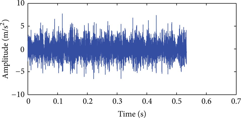
Time-domain waveform of fault signals of bearing outer race.

5.1. Complexity Mechanism of Single-Point Pitting of Bearing Outer Race

For faults of bearing outer race, the non-homogeneous load distribution will not produce a major impact on the fault signals of bearing outer race because the fault position remains unchanged in relation to that of the sensor. Therefore, the factor non-homogeneous load distribution is not represented in the formula. That is, x_l(t) ≈ 1, and the fault model of the bearing outer ring can be expressed as

X (t) = x_{f} (t) * y (t) + n (t) .

(16)

For the fault signal of bearing outer race, with the increase of fault severity, the width of each pulse sequence x_f(t) generated by faults also increases. For this reason, the duration of large-amplitude vibration of bearing signals will increase and become fuzzy due to overlapping. As the fault severity increases, the impact components of periodic pulse of the bearing vibration signal will be weakened continuously, with an increase in the disorder degree of the vibration signal. This will enhance the randomness of vibration signal X(t) distribution in the same time domain.

Figures 3 and 4 show the experimental vibration signals (the signals get by PCB-601 A02 acceleration sensor) of bearing faults at low and high fault severity, respectively. The experimental waveforms indicate that when the bearing fault is less severe, each impact component of the time-domain waveform has clearly divided boundary. However, when the fault is severe, the impact components overlap with each other, causing the vibration signals to become disordered and similar to random signals, with higher complexity. We can see the fault signals of bearing at high severity resemble random signals. However, the periodicity of bearing vibration signals at low severity degree is more apparent, with less randomness.

Figure 3:

Time-domain waveform for bearing outer race at low fault severity.

Figure 4:

Time-domain waveform for bearing outer race at high fault severity.

From the analysis above, we can predict that as the fault severity increases, Lempel-Ziv complexity of bearing outer race fault increases. And we will use experiments in part 6 to verify this conjecture.

5.2. Complexity Mechanism of Single-Point Pitting of Bearing Inner Race

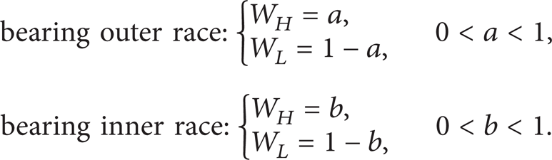
When there is single-point pitting damage in bearing inner race, modulated signals generated by non-homogeneous load distribution will have a strong impact on fault signals of bearing inner race because the inner race rotates when the bearing rotates and the fault position changes in relation to that of the sensor. Non-homogeneous load distribution under single-point pitting damage of bearing inner race cannot be ignored. Thus, the vibration signal model for single-point pitting damage of bearing inner race can be expressed by (14).

For a fault signal of bearing inner race, non-homogeneous load distribution (Figure 5) plays a very important role in vibration signals. With vibration value corresponding to the non-homogeneous load distribution x_l(t), a low-frequency amplitude modulation is generated. As fault severity increases, the pulse width also increases. The combined effect of pulse and non-homogeneous load distribution will enhance the periodicity of signal envelope, that is, enhance the signal modulation effect. Therefore, the modulation effect generated by non-homogeneous load distribution is dominant among the four vibration components for fault signals of bearing inner race. The signal envelope will show more apparent periodicity. With the increase of fault severity, the periodicity becomes increasingly apparent, which means that signal orderliness is enhanced while the complexity is reduced. Figure 6 is the simulated curves of the non-homogeneous load distribution obtained according to its variation pattern. It is easy to see that the non-homogeneous load distribution is periodic.

Figure 5:

Distribution of load areas.

Figure 6:

Simulated curve of non-homogeneous load distribution.

Figures 7 and 8 show experimental vibration signals (the signals gotten by PCB-601 A02 acceleration sensor) of bearing inner race at low and high fault severities, respectively. The experimental waveforms indicate that when the fault severity is low, the periodicity of time-domain waveform envelope is not so apparently; however, the periodicity of envelope increases while its complexity decreases at high fault severity.

Figure 7:

Time-domain waveform for bearing inner race at low fault severity.

Figure 8:

Time-domain waveform for bearing outer race at high fault severity.

From the analysis above, we can predict that as the fault severity increases, Lempel-Ziv complexity of bearing inner race decreases. And we will use experiments in part 6 to verify this conjecture.

5.3. Determination of Overall Lempel-Ziv Complexity

From the analysis above, it can be known that the vibration signal composition of bearing fault is very complex, the information of fault degree contained low-frequency and high-frequency components. Therefore the complexity needs to be calculated from low and high frequencies, respectively, after signal decomposition to ensure computation accuracy.

The overall complexity of the bearing can be expressed as the sum of high-frequency complexity C_nNH and low-frequency complexity C_nNL obtained according to the proportion. The computation equation is as follows:

C_{n} = W_{H} C_{n N H} + W_{L} C_{n N L},

(17)

where W_H and, W_L are the weight coefficients of high and low frequencies (W_H + W_L = 1), and the values of W_H and W_L are important factors to affect the Lempel-Ziv complexity calculation result. In order to get good calculation effect, we have to use more appropriate W_H and W_L according to the complexity theory of bearing.

In this paper we divided bearing fault signal into four parts: pulse sequence generated by fault (low frequency), modulation effect caused by the non-homogeneous load distribution (low-frequency), the attenuated natural vibration signal (high-frequency) and various undesired signals generated by other parts of the machine and noise (high frequency), as shown in Table 1. Except the noise component, other three parts have great relevance with bearing fault degree.

After the experiment and the analysis of the mechanism of bearing fault signal, as the fault severity increases in the outer race of bearing, the component of pulse sequence generated by the fault (low frequency) and the attenuated natural vibration signal (high frequency) must taken change. As a result, for outer race diagnosis, the highfrequency and low frequency all contains fault degree information. At this time the values of W_H and W_L could be set to 0.5 and 0.5.

But when the fault severity increases in the inner race of bearing, the component of the non-homogeneous load distribution (low frequency) taken change because the inner race rotates when the bearing rotates and the fault position changes in relation to that of the sensor. The pulse sequence generated by the fault (low frequency) and the attenuated natural vibration signal (high frequency) must taken change as well. As a result, for inner race diagnosis, with the low frequency containing more fault degree information, we should promote the proportion of low frequency when calculating the complexity. At this time the value of W_H and W_L could be set to 0.4 and 0.6.

The values of W_H and W_L can be calculated using the following equations:

\begin{matrix} bearing outer race: {\begin{cases} W_{H} = a, \\ W_{L} = 1 - a, \end{cases} 0 < a < 1, \\ bearing inner race: {\begin{cases} W_{H} = b, \\ W_{L} = 1 - b, \end{cases} 0 < b < 1 . \end{matrix}

(18)

According to the analysis above, the values of a and b could be set to a = 0.5 and b = 0.4.

In part 6, experiments could be used to verify the correctness of the interpretation and conjecture above.

6. Analysis of Experimental Data of the Rolling Bearing

Rolling bearing experiment is performed on the experiment platform in our laboratory to acquire the vibration signals in the operation process of bearing. The model of the experiment platform is shown in Figure 9.

Figure 9:

Experiment platform model.

Three-phase asynchronous motor ① is connected to the spindle equipped with rotors ④ via flexible coupling ②; the spindle is supported by two bearings of 6307. ③ is a normal bearing and ⑤ is a bearing with different modes of pitting damage (electric spark machining). The experimental acquisition system is composed of the main experiment platform, PCB-601A02 acceleration sensor, and PCI-4472 data acquisition card.

To identify the evolutionary process of bearing fault severity, single-point pitting damages with diameters of 0.5, 2, 3.5, and 5 mm on bearing inner race and outer race are made, respectively. During the experiment, the rotation speed of the motor is R = 1496 R/min, and sampling frequency f_s = 15360 Hz; number of sampling points n = 8192. One hundred sets of data are acquired for each pitting damage group and 10 sets of data are randomly selected to calculate the value of complexity.

The experiment's analysis focuses on the choice of time-frequency analysis method, the selection of optimum analysis area indices, and the values of the weight coefficients of high and low frequency complexity coefficient in the calculation of ultimate Lempel-Ziv complexity value. Wavelet analysis, EMD method and wavelet packet method are, respectively, used to choose the best time-frequency analysis method. Kurtosis and entropy indices are compared to select the best index of confirming the optimum analysis area. In the calculation of ultimate Lempel-Ziv complexity value, the coefficients value need to be analyzed and compared. The process is shown as in Figure 10. In order to make the result more reasonable, we select 10 sets of data from each kinds of damage randomly to calculate the average value of complexity.

Figure 10:

The analysis process of experiment.

6.1. The Comparison of the Time-Frequency Analysis Method

In order to verify the validity of the 3 time-frequency analysis method used in Lempel-Ziv complexity, signal decomposition is performed by wavelet analysis, EMD method, and wavelet packet method. The optimal area is selected using kurtosis index. a = 0.5 and b = 0.4 in the calculation of the overall Lempel-Ziv complexity of bearing. (The fault-complexity relationship is obtained by (17) and (18)).

According to the experimental results, the fault-complexity relationship curves obtained by continuous wavelet transform, EMD method, and wavelet packet method are plotted as shown in Figures 11 and 12, respectively, the abscissa represents the diameter of the damage (fault severity), the ordinate represents the Lempel-Ziv complexity, and the curve expresses Lempel-Ziv complexity variation with fault increase. All the three methods obtain the same results: as the fault severity increases, Lempel-Ziv complexity of bearing inner race decreases and that of bearing outer race fault increases. This law illustrates that the three methods are effective in terms of bearing failure degree diagnosis. However, the variation rate of Lempel-Ziv complexity of bearing inner race with fault severity is slower than that of bearing outer race. This phenomenon can be explained by complexity theory of bearing; the complexity mechanism of bearing shows that for fault signals of both bearing inner and outer races, the width of periodic pulses generated by faults will increase with fault severity, which will increase signal randomness and increase complexity. For fault signals of bearing inner race, modulated signals generated by non-homogeneous load distribution are dominant among the four vibration components. This makes the complexity decrease with increasing fault severity. The two reasons work together, resulting in less obvious variation trend of complexity of fault signals of bearing inner race.

Figure 11:

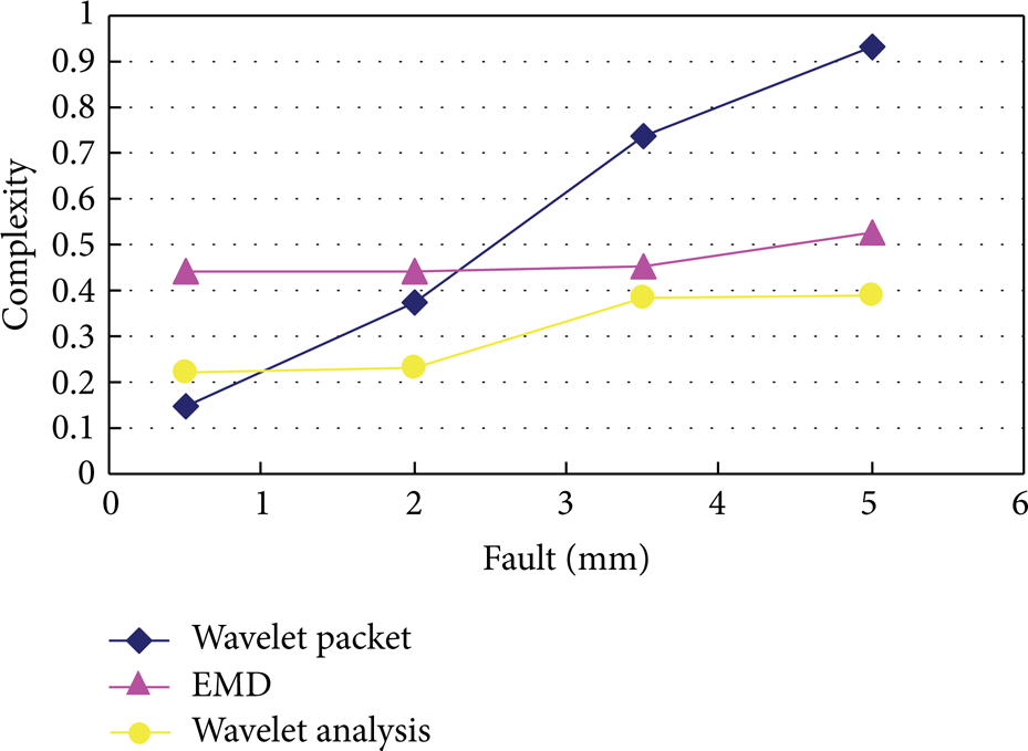
Comparison of complexity-fault curves obtained using wavelet packet method, wavelet analysis, and EMD method for signal decomposition in bearing outer race.

Figure 12:

Comparison of complexity-fault curves obtained using wavelet packet method, wavelet analysis, and EMD method for signal decomposition in bearing inner race.

The complexity-fault curves obtained using wavelet packet, wavelet analysis, and EMD method for signal decomposition are compared, respectively. In the case of fault in bearing inner race, as shown in Figure 12, the three methods get similar effects. In the case of fault in bearing outer race, as shown in Figure 11, with the increase of fault severity, the complexity-fault curve obtained by using the wavelet packet method to divide the analytical area shows the most obvious increasing trend. Therefore, under the experimental conditions of this paper, the wavelet packet method has higher differentiation of signals and efficiency in complexity analysis.

6.2. The Comparison of the Selection of Optimum Analysis Area Indices

In order to verify the validity of the 2 optimum analysis area indices used in Lempel-Ziv complexity, the optimal area is selected using kurtosis and entropy indices. Here wavelet packet method is used for signal decomposition. a = 0.5 and b = 0.4 in the calculation of overall Lempel-Ziv complexity of bearing (in the case of fault in bearing outer race).

The results obtained are shown in Figure 13; the abscissa represents the diameter of the damage (fault severity), the ordinate represents the Lempel-Ziv complexity, the curve expresses Lempel-Ziv complexity variation with fault increase. The curve obtained using kurtosis value to select the optimal area shows the expected variation trend; however that obtained using entropy value shows a U-shaped variation trend, which cannot reflect the fault severity. Therefore, kurtosis value is effective in terms of optimal area is selection, but entropy value is not. It is better to use kurtosis value than entropy value to select the optimal area.

Figure 13:

Comparison between the two methods.

6.3. The Selection of the Value of the Coefficients

This section is to verify that weight coefficients of high and low frequencies should be different and obtain the optimal values of a and b for a better calculation effect of complexity. The initial values of a and b in the experiment are set as 0.1. A group of overall Lempel-Ziv complexity values is calculated by (17) and (18). Then the overall Lempel-Ziv complexity value is obtained repeatedly by varying the values of a and b at the step length of 0.1. Finally, ten groups of overall Lempel-Ziv complexity values are calculated as the values of a and b varying from 0.1 and 0.2 to 1, and complexity-fault relationship curves are plotted, respectively. The optimal values of a and b are determined by comparing the variation trend of the curves.

Figures 14 and 15 show the comparison between the complexity-fault relationship curve when a = 0.1 to a = 1 and that when b = 0.1 to b = 1; the abscissa represents the diameter of the damage (fault severity), the ordinate represents the Lempel-Ziv complexity, the curve expresses Lempel-Ziv complexity variation with fault increase under different values of a and b. Here wavelet packet method is used for signal decomposition, and the optimal area is selected by kurtosis index.

Figure 14:

Complexity-fault relationship curves at different values of a for bearing outer race.

Figure 15:

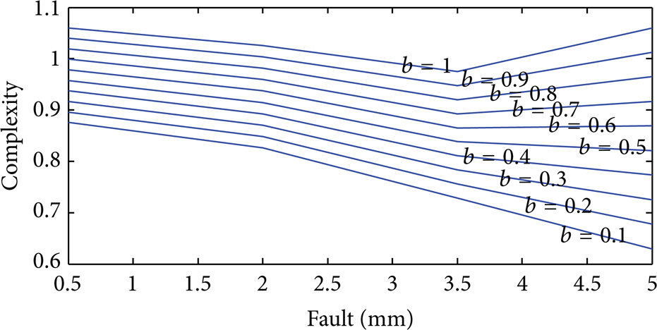
Complexity-fault relationship curves at different values of b for bearing inner race.

Figure 14 shows complexity-fault relationship at different values of a for bearing outer race; as the fault severity increases, Lempel-Ziv complexity of bearing outer race fault increases no matter what the value of a is. This law illustrates that all values of a are effective in terms of bearing failure degree diagnosis. However, we can find that the curve in Figure 14 is approximate straight line only when a = 0.5 or a = 0.6, and it is simpler to predict fault degree by using straight line than curve line. Therefore setting a = 0.5 or a = 0.6 could give the best result.

Figure 15 shows complexity-fault relationship at different values of b for bearing inner race; when the value of b is less than 0.4 or equal to 0.4, the Lempel-Ziv complexity of bearing inner race fault decreases as the fault severity increases; however that obtained using the value of b greater than 0.4 shows a U-shaped variation trend, which cannot reflect the fault severity. This result illustrates that only when the value of b is less than 0.4 or equal to 0.4 it is effective in terms of bearing failure degree diagnosis. However, we can find the curve in Figure 15 is approximate straight line only when b = 0.3 or b = 0.4, and it is simpler to predict fault degree by using straight-line than curve-line. Therefore setting b = 0.3 or b = 0.4 could give the best result.

The experimental results show the optimal values of weight coefficients in calculation of Lempel-Ziv complexity. Moreover, the results verified the explanations of Lempel-Ziv complexity theory of bearing in part 5.

7. Conclusions, Results, and Discussion

This paper presents a comparison of the effects of wavelet analysis, EMD, and wavelet packet method in vibration signal decomposition gotten by acceleration sensor for complexity calculation in quantitative fault diagnosis of bearing. We analyze the advantages and disadvantages of using kurtosis and entropy indices in optimal area selection and also explain and improve the selection of Lempel-Ziv complexity for high- and low-frequency signals. In addition, through the analysis of generation mechanism of bearing fault, the reasons for the changes in complexity of fault signals of bearing are investigated by considering the physical meaning of Lempel-Ziv complexity.

The following conclusions are reached through experimental analysis.

It is suitable for observing the fault growing trend and severity by examining the value based on improved Lempel-Ziv complexity algorithm using continuous wavelet transform (CWT), Empirical Mode Decomposition (EMD) method, and wavelet packet method for signal decomposition. Similar variation trend of complexity can be predicted: as the fault severity increases, the complexity of fault signals of bearing inner race decreases and that of bearing outer race increases. However, the variation rate for bearing inner race is slower than that for bearing outer race.

It is better to use kurtosis index than entropy index for optimal area selection.

For outer race diagnosis, the high frequency and low frequency all containing fault degree information, and for inner race diagnosis, the low frequency contain more fault degree information. The differentiation of complexity for different components can be adjusted by changing the complexity coefficients of bearing outer and inner races a and b. Optimal results can be obtained when a = 0.5 or a = 0.6 and b = 0.3 or b = 0.4.

Footnotes

Acknowledgments

This work is supported by the National Natural Science Foundation of China (Grant no. 50805001, 51175007, and 51075023), Beijing Science & Technology Star Plans (2008A014) Funding Project for Academic Human Resources Development in Institutions of Higher Learning Under the Jurisdiction of Beijing Municipality (PHR20110803), and Program for New Century Excellent Talents in University (NCET-12-0759).

References

Zhang

Asakura

, and Xu

, “Fault diagnosis system for rotary machine based on fuzzy neural networks,” JSME International Journal, Series C, vol. 46, no. 3, pp. 1035–1041, 2003.

Dong

G. M.

and Chen

, “Damage extent identification of rolling element bearings based on cyclic energy indicator,” Journal of Vibration Engineering, vol. 23, no. 3, pp. 249–253, 2010 (Chinese).

Feng

Zhengjia

, and Xuefeng

, “Operational reliability evaluation of machinery considering component damaged severity,” Journal of Xi'an Jiaotong University, vol. 44, no. 1, pp. 36–40, 2010 (Chinese).

Pan

Chen

, and Li

, “Bearing performance degradation assessment based on lifting wavelet packet decomposition and fuzzy c-means,” Mechanical Systems and Signal Processing, vol. 24, no. 2, pp. 559–566, 2010.

Lindh

Ahola

Spatenka

, and Rautiainen

A.-L.

, Automatic Bearing Fault Classification Combining Statistical Classification and Fuzzy Logic, Lappeenranta University of Technology, Lappeenranta, Finland, 2004.

Hong

and Liang

, “Fault severity assessment for rolling element bearings using the Lempel-Ziv complexity and continuous wavelet transform,” Journal of Sound and Vibration, vol. 320, no. 1–2, pp. 452–468, 2009.

Ruige

and Yonghong

, “A novel fault diagnosis for rolling element bearings based on continuous wavelet transform and hidden Markov model,” Applied Mechanic and Materials, vol. 109, pp. 313–317, 2012.

Dongyang

and Yingkai

, “Fault severity assessment for rolling element bearings based on EMD and Lempel-Ziv index,” Journal of Vibration and Shock, vol. 29, no. 3, pp. 5–8, 2010 (Chinese).

Jianxin

Husheng

Lushan

, “Study on fault diagnosis for rolling bearing based on EMD complexity feature and SVM,” Journal of Mechanical Transmission, vol. 2, pp. 20–23, 2011 (Chinese).

10.

Wensheng

Fengtao

Zhixin

Guo

Z. G.

, and Li

H. K.

, “Application of EMD denoising and spectral kurtosis in early fault diagnosis of rolling element bearings,” Journal of Vibration and Shock, vol. 29, no. 3, pp. 18–21, 2010 (Chinese).

11.

Ziv

and Lempel

, “A universal algorithm for sequential data compression,” IEEE Transactions on Information Theory, vol. 23, no. 3, pp. 337–343, 1977.

12.

Ziv

and Lempel

, “Compression of individual sequences via variable-rate coding,” IEEE Transactions on Information Theory, vol. 24, no. 5, pp. 530–536, 1978.

13.

Lempel

and Ziv

, “On the complexity of finite sequences,” IEEE Transactions on Information Theory, vol. 22, no. 1, pp. 75–81, 1976.

14.

Jianguo

, Wavelet Analysis and Engineering Applications, China Machine Press, Beijing, China, 2005.

15.

Huang

N. E.

Shen

Long

S. R.

, “The empirical mode decomposition and the Hilbert spectrum for nonlinear and nonstationary time series analysis,” Proceedings of the Royal Society of London A, vol. 454, pp. 903–995, 1998.

16.

Fulei

, Modern Signal Processing Methods in the Diagnosis of Mechanical Failure, Science Press, Beijing, China, 2009.

17.

Nikolaou

N. G.

and Antoniadis

I. A.

, “Demodulation of vibration signals generated by defects in rolling element bearings using complex shifted Morlet wavelets,” Mechanical Systems and Signal Processing, vol. 16, no. 4, pp. 677–694, 2002.

18.

Coifman

R. R.

and Wickerhauser

M. V.

, “Entropy-based algorithms for best basis selection,” IEEE Transactions on Information Theory, vol. 38, no. 2, pp. 713–718, 1992.

19.

L. I.

and Ming

, “Research on fault severity evaluation method for rolling bearings,” Bearing, vol. 4, pp. 42–46, 2009 (Chinese).

20.

Shannon

E. C.

, “A mathematical theory of communication,” Bell System Technical Journal, vol. 27, no. 3, pp. 379–423, 1948.

21.

Liangsheng

, Mechanical Fault Diagnosis Theories and Methods, Xi'an Jiaotong University Press, Xi'an, China, 2001.

22.

Hongbin

, Rolling Bearing Vibration Detection and Diagnosis, Machine Press, Beijing, China, 1995.