Sage Journals: Discover world-class research

Abstract

Data collection is one of the most important operations in wireless sensor networks. Currently, many researches focus on using a connected dominating set to construct a virtual backbone for data collection in WSNs. Most researchers concentrate on how to construct a minimum connected dominating set because a small virtual backbone incurs less maintenance. Unfortunately, computing a minimum size CDS is NP-hard, and the minimum connected dominating sets may result in unbalanced energy consumption among nodes. In this paper, we investigate the problem of constructing an energy-balanced CDS to effectively preserve the energy of nodes in order to extend the network lifetime in data collection. An energy-balanced connected dominating set scheme named DGA-EBCDS is proposed, and each node in the network can effectively transmit its data to the sink through the virtual backbone. When constructing the virtual backbone in DGA-EBCDS, we prioritize selecting those nodes with higher energy and larger degree. This method makes the energy consumption among nodes more balanced. Furthermore, the routing decision in DGA-EBCDS considers both the path length and the remaining energy of nodes in the path; it further prolongs the lifetime of nodes in the backbone. Our conclusions are verified by extensive simulation results.

1. Introduction

Wireless sensor network (WSN) is a new hot spot in current research, and it has broad application foreground [1, 2]. A wireless sensor network consists of a large number of nodes that collaborate together to monitor various phenomena. WSN can be used in various fields, such as battlefield, environment monitoring, disaster forecasting, business, and traffic control.

However, the communication ability, computational ability, storage ability, and energy of sensor nodes are limited [3–6], and the nodes are difficult to be replaced because they are often deployed in remote or inaccessible environments; the limitations of wireless sensor networks also shorten the performance of the network. Because of the limited energy, the signal generated by a source can only reach the nodes that are within its transmission range. If two nodes are within the transmission range of each other, they can exchange messages directly; otherwise, the messages have to be relayed through other intermediate nodes [7, 8]. This problem motivates us to construct a virtual backbone in wireless sensor network, and through this virtual backbone each node of the network can effectively transmit its data to the sink.

Wireless sensor networks (WSNs) are data oriented and are usually densely deployed in a monitor environment to process a great deal of data. Data collection is one of the most important operations in wireless sensor networks [9–13], which means that the data sensed by nodes should be transmitted to the sink for further processing. How to conserve the limited energy of nodes and extend the lifetime of the network is an important issue in data collection [14, 15]. The network lifetime is usually defined as the duration of the network until the first node depletes its energy. So, the network lifetime effectively ends with the first node death (FND). Due to incomplete data, the remaining energy in the surviving nodes is of no use after FND. In order to effectively extend the lifetime of a WSN (delay the death of the first node), many algorithms construct a virtual backbone of the network and only use the nodes in the virtual backbone to receive and transmit data for data collection. Nodes that are not in the backbone can go to sleep mode periodically to conserve the limited energy. Because of the number of nodes in the virtual backbone is relatively small, the impact of the broadcast storm problem can be greatly reduced, and the routing path search space can also be limited to the nodes that are in the set of the backbone. So, the virtual backbone can bring several benefits to network management.

Connected dominating set (CDS) plays an important role in the construction of virtual backbone in wireless sensor networks [16]. A dominating set (DS) of a network is a subset of all its nodes, which makes every node out of the set adjacent to at least one node in the set. A dominating set is called a connected dominating set when the nodes in the dominating set can form a connected graph. A CDS can be used as a virtual backbone to help each node transfer its data to the sink. Many researches focus on finding the minimum connected dominating set (MCDS) to construct the network virtual backbone [10]. However, MCDS-based algorithms may result in too much energy consumption of nodes in the backbone, and may cause unbalanced energy consumption among all the nodes, which will shorten the network lifetime and narrow their applications.

Motivated by the above problem, an energy-balanced connected dominating set scheme (DGA-EBCDS) is proposed in this paper, which well balances energy consumption among nodes that are in the backbone and consequently prolongs the lifetime of the network. In DGA-EBCDS, we prioritize selecting nodes that have higher energy and larger degree to form the backbone. By transmitting data through the backbone with small routing cost, each node can preserve its energy effectively. Moreover, the nodes in the virtual backbone would not die quickly because of their high energy level. The proposed algorithm creates a small-size connected dominating set, which performs well in energy saving and efficiently affords more numbers of rounds in data collection.

The main contributions of this paper are summarized as follows.

First, we introduce the concept of energy-balanced connected dominating set in Section 3. Using this scheme, DGA-EBCDS can well balance energy consumption among nodes and consequently prolong the lifetime of the network.

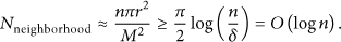
Second, we theoretically analyze DGA-EBCDS algorithm in Section 4. Theoretical analyses prove that the set of the dominators is a maximal independent set (MIS) when the first stage for DGA-EBCDS terminates and the message complexity of DGA-EBCDS is $O (n \log n)$ .

Third, we support our algorithm analysis with extensive simulations in Section 5. Compared with another dominating set-based algorithm mr-CDS [17], the average energy consumption of DGA-EBCDS is reduced by 33.3% in the formation of CDS, and the network lifetime is prolonged by 57.8%.

The rest of the paper is organized as follows. In Section 2, we briefly introduce the related work. Section 3 presents the system model and problem statement. In Section 4, we describe and analyze the proposed DGA-EBCDS protocol in detail. The simulation results and corresponding discussions are given in Section 5. Finally, Section 6 concludes the paper and presents the further research work.

2. Related Work

The construction of connected dominating set in wireless networks has been extensively studied for many years. In order to measure the quality of a connected dominating set, the size of the CDS is usually chosen as the main concern factor. A smaller CDS can suffer less interference from its neighbors because each node in a WSN shares the communication channel with its neighbors. Moreover, a smaller CDS can perform well in reducing the number and the cost of control messages in routing and transmission. On the other hand, the smaller CDS can also make the management of the virtual backbone easier. Based on the above reasons, many researches focused on reducing the size of a CDS [18–31]. Dai and Wu [18] firstly introduced two greedy algorithms to computer the MCDS in a generalG; both of them were polynomial time algorithms. Some works [18–20, 22] focused on constructing k-connected m-dominating sets for fault tolerance, and most of these works used a UDG as their network model. Wu et al. [23] proposed a CDS construction algorithm using an energy model which was also adopted in other works [24, 25]. Cardei et al. [26] and Funke et al. [27] proposed another two distributed algorithms, which could achieve better performance. Authors in [28–30] presented a distributed algorithm for constructing CDSs in UDGs, which consisted of two phases. Thai et al. [31] addressed the problem of constructing a CDS in a heterogeneous network and presented two approximation methods to obtain MCDS. Reference [21] considered constructing CDS in heterogeneous network, which formed an energy-efficient virtual network by using directional antennas. These algorithms effectively reduced the backbone size and improved the performance of the network.

Besides these algorithms, there were many other CDS-based algorithms aiming at the optimization goal of reducing the energy consumption of nodes in order to make the network live longer. CDS-BD-D [32] considered how to construct diameter restricted minimum connected dominating set. The diameter referred to the maximum length of the shortest path between any two nodes in the CDS. Data collection could be finished in limited delays by constructing diameter-restricted MCDS. GOC-MCDS-D [33] considered the routing cost of nodes and achieved higher energy efficiency than CDS-BD-D. Wu_h [34] aimed at creating the minimum connected dominating set and ignored the diameter size of the CDS. Another classic protocol named mr-CDS [17] considered the residual energy of nodes and effectively improved the energy efficiency of Wu_h [34]. Firstly, the node with higher residual energy than its neighboring nodes had a higher priority to become the dominator node. The selected dominator broadcasted its dominant message to its neighbors. The dominatee nodes could infer the number of the dominators among their neighbors from these dominant messages. Then, each node that was not in the dominating set would broadcast its neighbors' dominating set, which enabled the 2-hop neighbors of the dominators to know the dominators. By comparing the set of the 2-hops neighbors, each dominatee node could judge if there were any paths for the 2-hop dominator nodes. If no path existed to connect the dominator nodes, the node itself would become a dominator node. Finally, all dominator nodes would form a connected dominating set. However, the process of a dominatee node changing to a dominator node could not consider the energy factor, and each dominatee node autonomously converted to a dominator node, which made too many dominatee nodes change to dominator nodes at the same time. This caused the nodes consuming too much energy to run the pruning algorithm so as to reduce the number of nodes in the CDS. The message complexity of mr-CDS is $O (n \log n)$ . Since mr-CDS is very easy and effective, we will compare this classic protocol with our protocol in this paper.

Moreover, there were some other algorithms aiming at the optimization goal of ensuring the reliability of the network. That is to say, the data could still be transmitted to the sink after the death of some nodes. LDA [35] focused on how to structurek-connected m-dominating set, and each dominator node constructed a local k vertex-connected subgraph according to the neighbor information. Then, each dominator node noticed the dominate nodes in this subgraph to join the CDS. FT-CDS-CA [36] studied the problem of constructing fault-tolerant CDS and proposed a constant factor polynomial time approximation algorithm to compute (3, m)-CDS, which was similar to the method used in [22]. SSC [37] was the first self-stabilizing distributed (k, r) algorithm, which used synchronous multiple paths to improve security, availability, and fault tolerance of the algorithm.

3. System Model and Problem Statement

3.1. Network Model

Assume that there are n sensor nodes in the network that are labeled as $v_{1}, v_{2}, \dots, v_{n}$ , respectively. Denote the sink by $v_{0}$ . All the nodes are randomly deployed in a $M \times M$ field to continuously monitor the environment. Denote the transmission range of sensor nodes as r. We assume that $r ≪ M$ . The sink and all the sensor nodes form a connected network. Let V be the set of nodes. $| V |$ represents the number of nodes in set V, so, $| V | = n + 1$ . The network has the following characteristics: (1)

The network is static; that is, all nodes and the sink are stationary after deployment.

(2)

Nodes may have different initial energy. The sink is assumed to have infinite power supply and powerful computation ability.

(3)

Nodes are not aware of their geographic information.

(4)

Data are highly correlated; the nodes in the virtual backbone (the nodes in the CDS) can aggregate the data into one packet of k bits for transmission no matter how much data are arriving. The data aggregation makes the node able to merge its own data with the received data from its neighbors, leading to significant energy and bandwidth savings.

In this paper, we consider a wireless sensor network where data is periodically reported from the sensor nodes to the sink. Data collection and transmission proceeds in rounds, the data from the sensor nodes are collected and aggregated with the packets of peer sensor nodes, and only one data is sent per round from the sensor network to the sink, so, each node has only one packet of information to communicate in each round. A round is defined as the process of collecting all the data from nodes to the sink, regardless of how much time it takes [38].

3.2. Energy Model

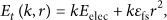
DGA-EBCDS uses the same energy consumption model which is widely adopted in previous works [39, 40]. According to this model, the energy dissipated to deliver a packet of k bits from the source to the destination is defined as

\begin{matrix} E_{t} (k, r) = k E_{elec} + k ε_{fs} r^{2}, \end{matrix}

(1)

where

E_{elec}

is the energy dissipated in operating the transmitter radio, r is the transmission range of the node and

ε_{fs} r^{2}

represents the energy dissipated by transmitter amplifier which varies with the distance r between the two nodes. The energy dissipated in operating the receiver radio is expressed as

\begin{matrix} E_{r} (k) = k E_{elec} . \end{matrix}

(2)

3.3. Problem Statement

The minimum connected dominating set (MCDS) is an NP-hard problem for general graphs [41]. The MCDS can simplify network abstracted topology and reduce routing cost. However, when the nodes in the MCDS are without enough energy, these nodes will die earlier because of consuming energy too quickly.

Consider the graph shown in Figure 1(a). There are 7 nodes and one sink in the network, and each node starts with different amount of energy. A (1) represents node A having one unit of energy, and so forth.

Figure 1

Different CDS-generating approaches (blacked nodes represent dominators, shaded nodes represent connectors).

In Figure 1(b), network generates CDS only by node degree. B has the largest node degree, so it becomes a dominator (to be blacked) firstly. And the neighboring nodes of B (A, C, D, E, and F) become the dominatees. The left node G has no other nodes to compare with, so it becomes the dominator naturally. In order to connect two dominators G and B, F becomes the connector (to be shaded). So, CDS contains three nodes (B, F, and G), accounting for 43% of the total number of nodes, and there is only one path from the CDS to the sink; this path transmits all the data flows of the network; thus, the energy consumption of this path is very large.

In Figure 1(c), network generates CDS by node energy. E and G have larger energy, so they become dominators firstly, and then, A and F become the connectors to connect G and the sink, and C and D become the connectors to connect E and the sink. Thus, CDS contains six nodes, accounting for 86% of the total number of nodes. CDS as the virtual backbone has to work long hours and should not go to the sleep mode, so this part of the nodes will run out of energy quickly and die earlier.

In Figure 1(d), network generates CDS by two factors: both the energy and the degree of a node. F and D both have larger degree and higher energy, so they become dominators firstly, and then, A becomes the connector to connect F and the sink, and C becomes the connector to connect D and the sink. Thus, CDS contains four nodes, accounting for 57% of the total number of nodes. Meanwhile, there are two paths from the CDS to the sink; more nodes outside the CDS can go to the sleep mode, which can not only reduce the size of the CDS, but also balance the energy consumption among nodes and extend the network lifetime.

So, constructing an energy-balanced CDS is a good method to solve the problems of MCDS, which takes both the energy and the degree of a node into consideration so as to effectively prolong the network lifetime in wireless sensor network.

4. The Design and Analysis of DGA-EBCDS

For the sake of brevity in describing our algorithm in the following, we give some definitions and notations here. Let $N (v_{i})$ be the neighbors set of a node i. Dominators represent the nodes in the dominating set. Dominatees represent the nodes that are not in the dominating set. Connectors refer to the nodes that can connect two different dominators that are not adjacent to each other, and all the dominators and connectors can form a connected dominating set. Independent set (IS) is a subset of V such that no two vertices within the set are adjacent in V. Maximal independent set (MIS) is an independent set such that adding any vertex not in the set breaks the independence property of the set; thus, the number of the IS nodes in the MIS is the largest. Let $P (v_{i})$ be the set of neighboring nodes of node i that cannot become any kinds of dominators, dominates, or connectors. These definitions and notations will be used throughout this paper.

DGA-EBCDS is a distributed algorithm it depends only on the local information of nodes. The algorithm does not require the global information. DGA-EBCDS includes two stages: in the first stage, DGA-EBCDS selects the dominators; in the second stage, DGA-EBCDS selects the connectors, and finally, all the dominators and connectors form a CDS.

In order to construct an energy-balanced CDS, we use a weight $W_{i}$ to measure the capability of a node, $W_{i} = E_{i} {Degree}_{i}$ , where $E_{i}$ is the energy of node $v_{i}$ and ${Degree}_{i}$ is the degree of node $v_{i}$ . The higher the weight is, the more is its chance to become a dominator. By combining energy and degree together to measure the capability of a node, the node with a higher weight has higher priority to become a backbone node. That is to say, the node with more energy and larger degree has more chance to become a CDS node. In this section, we will describe the details of DGA-EBCDS as follows.

4.1. Construction of Energy-Balanced CDS

Sensor nodes in the DGA-EBCDS can have three different colors: “white,” “gray,” and “black”. Initially, all nodes are “white.” During the execution of our algorithm, all nodes change their color to either “black” or “gray.” Based on the weight comparison among neighbors, some suitable nodes are selected as dominators; nodes that are not in the dominating set remain as dominatees. All the black nodes form the dominating set (network backbone), whereas the gray nodes remain as dominatees, and they use neighboring dominators as next hops to transmit the data. Each node runs DGA-EBCDS distributedly and the algorithm includes the two following stages: (1)

Weight comparison among neighbors in the first stage, and some suitable nodes are selected as the dominators. During weight comparison, node i is more suitable to be a dominator than its neighboring j when node i has a higher weight than j, or the weights of node i and j are the same, but the ID of node i is smaller than that of node j. When a node i wins the weight comparison over its neighbors, the node i becomes the dominator and turns “black;” when its neighboring nodes receive the black message from node i, they will become dominatees and turn “gray.” Algorithm 1 gives detailed description of the selection of dominators by comparing the weights among nodes.

(2)

In the second stage, the dominators select the suitable neighbors to become the connectors, and then the dominating nodes can be connected by the connectors. The selection is decided on the energy level of their neighbors as well as the connection condition between the neighbors and other dominators. When node i becomes a connector, it will turn “black” too. Finally, all the dominators and connectors will form a connected dominating set (network backbone). We use two lists (List1 and List2) to save the path information. Algorithm 2 gives detailed description of the selection of connectors.

Algorithm 1: The first stage for DGA-EBCDS.

At the beginning of the first stage:

P( $v_{i}$ ) = N( $v_{i}$ );

if ( $W_{i}$ > max ${W_{j} ∣ v_{j} \in P (v_{j})}) ∥ ((W_{i} = =$ max ${W_{j} ∣ v_{j} \in P (v_{j})})$ && $(v_{i} = =$ min ${v_{i}, {v_{k} ∣ W_{k} =$ max ${W_{j} ∣ v_{j} \in P (v_{j})}}))$

{ $v_{i \cdot}$ color = “Black”;

$v_{i}$ broadcasts a message dominator( $v_{i}$ )

When $v_{i}$ receives a dominator ( $v_{k}$ ) message:

if ( $v_{i \cdot}$ color $= =$ “White”)

${v_{i \cdot}$ color = “Gray”;

$v_{i}$ broadcasts a message dominate( $v_{i}$ );}

When $v_{i}$ receives a dominate ( $v_{j}$ ) message:

if ( $v_{i \cdot}$ color $= =$ “White”)

{ delete $v_{j}$ from $P (v_{i})$ ;

if $(W_{i} >$ max ${W_{j} ∣ v_{j} \in P (v_{j})})$ $∥$ $((W_{i} = =$ max ${W_{j} ∣ v_{j} \in P (v_{j})})$ && $(v_{i} = =$ min ${v_{i}, {v_{k} ∣ W_{k} =$ max ${W_{j} ∣ v_{j} \in P (v_{j})}}))$

{ $v_{i \cdot}$ color = “Black”;

$v_{i}$ broadcasts a message dominator( $v_{i}$ ); $}}$

Algorithm 2: The second stage for DGA-EBCDS.

At the beginning of the second stage:

if( $v_{i \cdot}$ color $= =$ “Gray”)

for (each dominator $v_{k}$ that is one of the neighbors of $v_{i}$ )

$v_{i}$ broadcasts a message dominatee1( $v_{i}$ , $v_{k}$ );

When $v_{i}$ receives a dominatee1( $v_{j}$ , $v_{k}$ ) message:

if ( $v_{i \cdot}$ color $= =$ “Gray”)

{if (there is a dominator $v_{m}$ that is one of the neighbors of $v_{i}$ )&&( $v_{m} < v_{k}$ )

$v_{i}$ broadcasts a message dominatee2( $v_{i}$ , $v_{j}$ , $v_{k}$ );

}else if ( $v_{i \cdot}$ color $= =$ “Black”)

{if ((List1 $= =$ null) $∥$ ( $[v_{l}$ , $v_{k}]$ is not in List1))

{ add record $[v_{i}$ , $v_{k}]$ to List1;

$v_{i}$ waits to receive the dominatee1 and the dominatee2 messages sending from other neighbors;

}else if (there is a record $[v_{l}$ , $v_{k}]$ in List1 and $E_{l} < E_{j}$ )

{ delete $[v_{l}$ , $v_{k}]$ from List1;

add $[v_{j}$ , $v_{k}]$ to List1; $}}$

When $v_{i}$ receives a dominatee2( $v_{n}$ , $v_{j}$ , $v_{k}$ ) message:

if ( $v_{i \cdot}$ color $= =$ “Black”)

{if ((List2 $= =$ null) $∥$ ( $[v_{m}$ , $v_{l}$ , $v_{k}]$ is not in List2))

{add record $[v_{n}$ , $v_{j}$ , $v_{k}]$ to List2;

$v_{i}$ waits to receive the dominatee1 and the dominatee2 messages sending from other neighbors;

}else if (there is a record $[v_{m}$ , $v_{l}$ , $v_{k}]$ in List2)&&(min ${E_{m}$ , $E_{l}}$ < min ${E_{n}$ , $E_{j}}$ )

{delete $[v_{m}$ , $v_{l}$ , $v_{k}]$ from List2;

add $[v_{n}$ , $v_{j}$ , $v_{k}]$ to List2; $}}$

When the timer Timer expired:

for (each record $[v_{l}$ , $v_{k}]$ in List1)

{ add $v_{l}$ to a set A;

delete $[v_{n}$ , $v_{j}$ , $v_{k}]$ from List2;}

for(each record [ $v_{n}$ , $v_{j}$ , $v_{k}$ ] in List2)

{ add $v_{n}$ and $v_{j}$ to the set A;}

$v_{i}$ broadcasts a message connector (A, 2);

When $v_{i}$ receives a connector (A, a) message:

a = a-1;

If ( $v_{i} \in A$ )&&( $v_{i \cdot}$ color $= =$ “Gray”)

$v_{i \cdot}$ color = “Black”;

if ( $a \geq 1$ )

$v_{i}$ broadcasts a message connector (A, a);

In Algorithm 2, at the beginning of the second stage, if the color of node $v_{i}$ is “Gray,” $v_{i}$ will broadcast a message dominatee1( $v_{i}, v_{k}$ ) for each dominator $v_{k}$ that is one of the neighbors of $v_{i}$ ; this message will help $v_{i}$ to search for other dominators that $v_{i}$ can connect them through $v_{k}$ .

When $v_{i}$ receives a dominatee1( $v_{i}, v_{k}$ ) message, $v_{i}$ checks the color of itself; if the color of node $v_{i}$ is “Gray,” and if there is a dominator $v_{m}$ that is one of the neighbors of $v_{i}$ and $v_{m} < v_{k}$ , $v_{i}$ will broadcast a message dominatee2 $(v_{i}, v_{j}, v_{k})$ ; the message will make $v_{m}$ know that it can connect $v_{k}$ through $v_{i}$ and $v_{j}$ . If the color of node $v_{i}$ is “Black,” $v_{i}$ will wait to receive the dominatee1 and the dominatee2 messages being sent from other neighbors; otherwise, if there is a record $[v_{l}, v_{k}]$ in List1 and $E_{l} < E_{j}$ , delete $[v_{l}, v_{k}]$ from List1 and then add $[v_{j}, v_{k}]$ to List1.

When $v_{i}$ receives a dominatee2 $(v_{n}, v_{j}, v_{k})$ message, if the color of node $v_{i}$ is “Black,” and if List2 is empty or $[v_{m}, v_{l}, v_{k}]$ cannot be found in List2, add the record [ $v_{n}, v_{j}, v_{k}$ ] to List2; $v_{i}$ waits to receive the dominatee1 and the dominatee2 messages being sent from other neighbors; otherwise, if there is a record [ $v_{m}, v_{l}, v_{k}$ ] in List2 and $\min {E_{m}, E_{l}} < \min {E_{n}, E_{j}}$ , delete [ $v_{m}, v_{l}, v_{k}$ ] from List2; and then, add the record [ $v_{n}, v_{j}, v_{k}$ ] to List2.

When the timer expires, if $v_{i}$ can connect with $v_{k}$ through $v_{1}$ , add $v_{l}$ to a set A and delete the record [ $v_{n}, v_{j}, v_{k}$ ] from List2; if $v_{i} \in A$ and the color of node $v_{i}$ is “Gray,” $v_{i}$ will change itself from a dominatee to a connector, and then, the color of $v_{i}$ turns to “Black.”

Each node runs DGA-EBCDS distributedly; when a node turns to “Black,” it will never change its color again. At the end of the second stage, the set of “Black” nodes (dominators and connectors) forms a CDS.

4.2. Analysis of the Distributed Algorithm

Theorem 1.

The set of the dominators is a maximal independent set (MIS) when the first stage for DGA-EBCDS terminates.

Proof.

From the detailed description of the algorithm shown in Algorithm 1, all the nodes will make a weight comparison among neighbors in the first stage of DGA-EBCDS. During weight comparison, $v_{i}$ will be selected as a dominator when $v_{i}$ has a higher weight than its neighboring $v_{j}$ , or the weights of $v_{i}$ and $v_{j}$ are the same, but the ID of $v_{i}$ is smaller than that the ID of $v_{i}$ . When $v_{i}$ wins the weight comparison over its neighbors, it will become a dominator.

When $v_{i}$ becomes a dominator, all the neighbors of $v_{i}$ will become dominates; thus, each two dominators cannot be connected directly. From the above analysis, the set of all the dominators is an independent set (IS). For any node $v_{i} \in V$ , according to DGA-EBCDS, there are only two possible cases for $v_{i}$ : if $v_{i}$ is not a dominator, it must be a dominatee. For each dominatee, there is certainly at least one dominator in its neighbors. Therefore, any dominatee turning to a dominator will break the independence property of the current set (produce two dominators that can be connected directly). Thus, the set of the dominators is a maximal independent set (MIS) when the first stage for DGA-EBCDS terminates.

Theorem 2.

The message complexity of DGA-EBCDS is $O (n \log n)$ .

Proof.

In order to guarantee that the network is connected, the transmission radius of r should satisfy the following formula [42]:

\begin{matrix} r \geq \frac{\sqrt{2}}{2} M \sqrt{\frac{1}{n} \log (\frac{n}{δ})}, \end{matrix}

(3)

where δ represents the probability that the network is not connected. Certainly, the number of the neighboring nodes must satisfy

\begin{matrix} N_{neighborhood} \approx \frac{n π r_{}^{2}}{M^{2}} \geq \frac{π}{2} \log (\frac{n}{δ}) = O (\log n) . \end{matrix}

(4)

From the detailed description of the algorithms shown in Algorithms 1 and 2, for each node $v_{i}$ , if $v_{i}$ is a dominator, it will send two messages: one message for declaring itself being selected as the dominator and the other message for broadcasting the set of the connectors.

If $v_{i}$ is a dominatee, it will send at most $O (\log n)$ messages: one message for broadcasting dominatee $(v_{i})$ , $O (\log n)$ messages for broadcasting dominatee1 $(v_{i}, v_{j})$ , and $O (\log n)$ messages for broadcasting dominatee2 $(v_{i}, v_{j}, v_{k})$ , where $O (\log n)$ is decided by the number of the neighboring nodes of $v_{i}$ .

If $v_{i}$ turns out to be a connector, it will broadcast connector $(A, a)$ message only once.

Thus, a node will send at most $O (\log n)$ messages in DGA-EBCDS. There are n nodes in the network; we can deduce that the total message complexity of the network is $O (n \log n)$ , which is the same as the message complexity of the classic DS-based algorithm mr-CDS.

5. Performance Evaluation

We conduct extensive simulations to evaluate the performance of DGA-EBCDS. The experiments are assumed to be performed in a square field of $M \times M$ , in which nodes are randomly dispersed. The parameters are as follows.

Each node in the field is assigned a randomly-generated initial energy level between 1 joule(J) and 1.5 J, $E_{elec} = 50$ nJ/bit, $ε_{fs} = 13$ pJ/bit/m², and each node will generate only one packet of 1000 bits per round. We compare DGA-EBCDS with mr-CDS and use the same assumption of mr-CDS. Sink is located at the center of the field; its coordinate is $(0.5 M, 0.5 M)$ . All experiments will be performed 20 times, and their average values are taken as the final results. Our target is to balance the energy among nodes and delay the death of the first node. Network density is defined as the number of nodes lying in each unit of the field, which can be described as $n / M^{2}$ . Average node degree represents the number of nodes in its transmission range, which can be described as $n π r^{2} / M^{2}$ ; we will use them to set our experiment scenes.

5.1. Backbone Size

We simulate a network of 480 static nodes placed randomly in a 1000 m × 1000 m area to observe the distribution of the CDS. The transmission range of nodes is set to be 100 m. The simulation results are shown in Figure 2.

Figure 2

Backbone size comparison of DGA-EBCDS and mr-CDS.

In Figure 2, the sink is marked with a pentagram, the nodes in the CDS (including dominators and connectors) are marked with circles adding a plus sign, and dominatees are marked with circles. We can observe that the CDS produced by DGA-EBCDS and mr-CDS can both cover the whole network, which can effectively guarantee the network coverage.

In order to measure the validity of these two algorithms, we have used two different environments to randomly deploy the sensor nodes. Figures 2(a) and 2(b) are the first deployment environment, and Figures 2(c) and 2(d) are the second deployment environment.

We can see from Figures 2(a) and 2(b), in the first experiment, on average, 142 nodes constitute the mr-CDS backbone, whereas in case of DGA-EBCDS, there are only 79 nodes generated in the backbone; the backbone size of DGA-EBCDS is reduced by 44.4% on average.

Meanwhile, we can see from Figures 2(c) and 2(d), in the second experiment, on average, 146 nodes constitute the mr-CDS backbone, whereas in case of DGA-EBCDS, there are only 86 nodes generated in the backbone; the backbone size of DGA-EBCDS is reduced by 41.1% on average.

As backbone nodes must remain active during the network operating period, with fewer nodes in the backbone, DGA-EBCDS consumes less energy to keep the network in an operational state, and a smaller backbone in DGA-EBCDS can make more nodes (dominatees) go to a periodic sleep mode and effectively save the energy of the network. Moreover, no matter how the randomized sensor placements change, DGA-EBCDS always achieves better performance than mr-CDS.

5.2. Energy Consumption in the Formation of CDS

In order to compare the energy efficiency of DGA-EBCDS and mr-CDS, we have examined the average energy consumption per node in the formation phase of CDS. The transmission range of nodes is set to 100 m, and the message packets size of nodes is 32 bits. We have investigated both algorithms under varying conditions like average node degree and the scale of the network. Two experimental scenes are used: (1)

Scene 1: the area is fixed to 1000 m × 1000 m. Assume that there are 320, 480, 640, 800, and 960 nodes randomly distributed in the field, respectively. The average node degree is 10, 15, 20, 25, and 30 under this scene, respectively.

(2)

Scene 2: the average node degree is fixed to 15. The area is 800 m × 800 m, 1000 m × 1000 m, 1200 m × 1200 m, and 1500 m × 1500 m, respectively. There are 306, 480, 688, and 1075 nodes in this scene, respectively. The energy consumption in the formation phase of CDS is shown in Figure 3.

Figure 3

Energy consumption comparison of DGA-EBCDS and mr-CDS in the formation of CDS.

We can see from Figure 3(a), in the formation of CDS, the energy consumption of nodes increases when the average node degree grows. The reason is that nodes need to exchange messages with their neighbors. As the average node degree increases, the node needs to exchange its messages with more neighbors, which exhausts too much energy. However, DGA-EBCDS consumes less energy than mr-CDS; the average energy consumption has been reduced by 33.3%.

In Figure 3(b), when average node degree is fixed, the energy consumption for DGA-EBCDS and mr-CDS will be similar. Because the numbers of average neighbors of nodes will remain unchanged when average node degree is fixed, the energy consumption will be unchanged. However, DGA-EBCDS consumes less energy than mr-CDS in different scales of network. Based on the observation, we can get the conclusion that DGA-EBCDS considers the energy balancing among nodes, as a result, DGA-EBCDS wastes less energy and acquires better energy efficiency than mr-CDS.

5.3. Network Lifetime

We set the same scenes of section B to evaluate the network lifetime. The energy of node will be reducing in data collection and the energy is changing per round. Node broadcasts its energy message at the beginning of each round. The message of energy can be delivered by some small packets; the energy consumption of this part can be neglected in the network.

In wireless sensor networks, the energy of node is very limited, if the network lifetime (FND) expires, remaining energy of the alive nodes cannot come to any use. So our algorithm tries to maximize the use of overall network energy before a network expires and extend network lifetime by delaying the death of the first node. In the process of data collection, the node cannot acquire the path information, so it does not know from which path it can transmit its data to sink with less energy consumption. There are many algorithms using the nodes in the CDS to construct a data collection tree and set the sink as the root of the tree. We no longer specially discuss this method here, and we use the distance vector (DV) routing algorithm [43] to construct a data collection tree after forming a CDS-based backbone. The collection tree is also used by mr-CDS. The sink acts as the root node and initiates tree formation, and only the dominators take part in the construction of the tree. Furthermore, we can see from Figure 2 that the number of dominators of DGA-EBCDS is quite lower when compared to the network size, so running DV algorithm only over the dominators can reduce the cost of the network.

In the data collection process, each dominatee will transmit its data to the neighbor that has the highest energy in the data collection tree, and then it goes to the sleep mode to save its energy. The nodes in the data collection tree will aggregate the received data into one packet of 1000 bits and then transmit the packet to their father. A round of data collection terminates when the sink receives all the data from its children. Network lifetime achieved by these two algorithms is shown in Figure 4.

Figure 4

Network lifetime comparison of DGA-EBCDS and mr-CDS.

In Figure 4(a), the network lifetime is decreasing as the average node degree increases. DGA-EBCDS achieves longer network lifetime than mr-CDS no matter how the average node degree changes.

In Figure 4(b), when the average node degree is fixed, the network lifetime in large-scale network is shorter than that in small-scale network. As the transmission range is the same, the data need to be transmitted more times to get to the sink in large-scale network than in small-scale network, so the network lifetime in large-scale network will be reduced. However, DGA-EBCDS achieves longer network lifetime than mr-CDS. On average, the network lifetime is prolonged by 57.8%.

5.4. Delay

We set the same scenes of Section 5.2 to evaluate the data dissemination delays of these two algorithms. Since data dissemination delay are mainly affected by the maximum number of hops from the node to the sink, that is, the larger the number of hops, the longer the delay, we use the maximum number of hops between sink and the node to measure the data dissemination delay. The comparison results of data dissemination delay are shown in Figure 5.

Figure 5

Delay comparison of DGA-EBCDS and mr-CDS.

In Figure 5, we can see that the data dissemination delays are mostly influenced by the size of the network; however, the average node degree produces very little influence on data dissemination delays.

In Figure 5(a), the data dissemination delays of these two algorithms remain unchangeable as the average node degree increases. The average delay of DGA-EBCDS is 9.63 hops, and the average delay of mr-CDS is 8.36 hops. DGA-EBCDS incurs a larger delay (just only one hop on average) than that of mr-CDS.

In Figure 5(b), when the average node degree is fixed, the data dissemination delays of these two algorithms in large-scale network are larger than that in small-scale network. As the transmission range is the same, the data need to be relayed by more nodes to get to the sink in large-scale network than in small-scale network, so the data dissemination delays in large-scale network will be enlarged. The average delay of DGA-EBCDS is 10.49 hops, and the average delay of mr-CDS is 9.29 hops; mr-CDS shortens the delay by only one hop on average. Moreover, from Figure 2, we can see that the backbone size of DGA-EBCDS is smaller than that of mr-CDS. In some cases, there are fewer paths between the nodes and the sink, so some CDS nodes of DGA-EBCDS need to be transmitted more times to get to the sink; thus, DGA-EBCDS incurs larger delays than that of mr-CDS.

However, DGA-EBCDS considers the energy balancing among nodes. The algorithm can significantly delay the death of the first node, and the dominators can take more rounds for data collection. Based on the observation, we can draw the conclusion that DGA-EBCDS gains better performance than mr-CDS.

6. Conclusion and Future Work

Selecting proper nodes to construct the CDS in order to maximize the network lifetime is an important issue when designing connected dominating set protocols and algorithms for data collection in wireless sensor networks. Most existing algorithms cannot consider the energy balancing among nodes, which limits their applications in large scale WSNs. The high contribution of this paper is the construction of an energy-balanced connected dominating set (DGA-EBCDS) for data collection in wireless sensor network. DGA-EBCDS can effectively increase the number of rounds before the first node failure by reducing the energy consumption per round and only choosing the nodes with a relatively higher weight to construct the CDS. Theoretical analyses show that the total message complexity of the algorithm is $O (n \log n)$ , and the simulation results show that DGA-EBCDS can reduce energy consumption in the formation of CDS as well as effectively prolong the lifetime of the network.

In the next step, how to switch the role of dominators when designing the CDS backbone is a new research direction for us. If we always use the same set of dominators, those nodes must relay network traffic all the time, and they will easily run out of energy when compared with the dominatee nodes. We can consider that once the energy of a dominator goes below a threshold, a new node can take up the responsibility of this dominator. Therefore, researches that aim at delaying the death of the first node and switching the role of dominators can be useful in the future work.

Footnotes

Acknowledgments

This work is supported by the National Natural Science Foundation of China (Grant nos. 61202494, 61103245), the Scientific Research Fund of Hunan Provincial Education Department (Grant no. 11C1099), the Natural Science Foundation of Guangxi (Grant no. 2012GXNSFBA053163), Hunan Provincial Science and Technology Department projects (2010FJ4052), and the Freedom Explore Program of Central South University (2012QNZT068).

References

Chuang

P. J.

Y. C.

Lin

C. S.

Reliable and congestion-controlling transport in wireless sensor networks

Journal of the Chinese Institute of Engineers 2013 36 1 2 16

10.1080/02533839.2012.726021

Liu

A. F.

Zheng

Z. M.

Zhang

Chen

Shen

Secure and energy-efficient disjoint multi-path routing for WSNs

IEEE Transactions on Vehicular Technology 2012 61 7 3255 3265

Kimura

Jolly

Latifi

Energy restrained data dissemination in wireless sensor networks

International Journal of Distributed Sensor Networks 2006 2 3 251 265

2-s2.0-35348890997

10.1080/15501320600642692

Liu

A. F.

Liu

Z. H.

An elaborate chronological and spatial analysis of energy hole for wireless sensor networks

Computer Standards and Interfaces 2013 35 1 132 149

Lee

W. C.

Mitchell

Energy-aware and time-critical geo-routing in wireless sensor networks

International Journal of Distributed Sensor Networks 2008 4 4 315 346

2-s2.0-54249137727

10.1080/15501320701260410

Ota

Dong

Cheng

Wang

Shen

ORACLE: mobility control in wireless sensor and actor networks

Elsevier Computer Communications 2012 35 9 1029 1037

Zhu

Lin

Fan

Shen

SMART: a secure multilayer credit-based incentive scheme for delay-tolerant networks

IEEE Transactions on Vehicular Technology 2009 58 8 4628 4639

2-s2.0-70350238158

10.1109/TVT.2009.2020105

Zhu

Gao

Dong

Cao

A probabilistic misbehavior detection scheme towards efficient trust establishment in delay tolerant networks

IEEE Transactions on Parallel and Distributed Systems 2013

10.1109/TPDS.2013.36

Kui

X. Y.

Wang

J. X.

Zhang

S. G.

Energy-balanced clustering protocol for data gathering in wireless sensor networks with unbalanced traffic load

Journal of Central South University 2012 19 11 3180 3187

10.

Zheng

Sun

S. X.

Huang

T. Y.

Constructing distributed connected dominating sets in wireless Ad Hoc and sensor networks

Ruan Jian Xue Bao/Journal of Software 2011 22 5 1053 1066

2-s2.0-79959758235

10.3724/SP.J.1001.2011.00586

11.

Gao

Zhang

H. K.

Optimal path selection for mobile sink in delay-guaranteed sensor networks

Tien Tzu Hsueh Pao/Acta Electronica Sinica 2011 39 4 742 747

2-s2.0-79959707634

12.

Cai

Distributed data collection in large-scale asynchronous wireless sensor networks under the generalized physical interference model

IEEE/ACM Transactions on Networking 2012

10.1109/TNET.2012.2221165

13.

Cai

Distributed data collection and its capacity in asynchronous wireless sensor networks

Proceedings of the 31st Annual IEEE International Conference on Computer Communications (INFOCOM '12)

March 2012

Orlando, Fla, USA

2113 2121

14.

Liu

A. F.

Zhang

P. H.

Chen

Z. G.

Theoretical analysis of the lifetime and energy hole in cluster based Wireless Sensor Networks

Journal of Parallel and Distributed Computing 2011 71 10 1327 1355

15.

Liu

A. F.

Jin

Cui

G. H.

Chen

Z. G.

Deployment guidelines for achieving maximum lifetime and avoiding energy holes in sensor network

Information Sciences 2013 230 197 226

10.1016/j.ins.2012.12.037

16.

Pan

Cai

Approximation algorithms for load-balanced virtual backbone construction in wireless sensor networks

Theoretical Computer Science 2012

10.1016/j.tcs.2012.11.020

17.

Hussain

Shafique

M. I.

Yang

L. T.

Constructing a CDS-based network backbone for energy efficiency in industrial wireless sensor network

Proceedings of the 12th IEEE International Conference on High Performance Computing and Communications (HPCC '10)

September 2010

Melbourne, Australia

322 328

2-s2.0-78149350569

10.1109/HPCC.2010.96

18.

Dai

On constructing k-connected k-dominating set in wireless networks

Proceedings of the 19th IEEE International Parallel and Distributed Processing Symposium (IPDPS '05)

April 2005

Denver, Colo, USA

2-s2.0-33746307641

10.1109/IPDPS.2005.302

19.

Wang

Thai

M. T.

D. Z.

On the construction of 2-connected virtual backbone in wireless networks

IEEE Transactions on Wireless Communications 2009 8 3 1230 1237

2-s2.0-62949148901

10.1109/TWC.2009.051053

20.

Wang

Thai

M. T.

Constructing k-connected M-dominating sets in wireless sensor networks

Proceedings of the Military Communications Conference (MILCOM '07)

October 2007

1 7

2-s2.0-47949083311

10.1109/MILCOM.2007.4454774

21.

Yang

Dai

Efficient backbone construction methods in MANETs using directional antennas

Proceedings of the 27th International Conference on Distributed Computing Systems (ICDCS '07)

June 2007

45 50

2-s2.0-34848839871

10.1109/ICDCS.2007.105

22.

Thai

M. T.

Zhang

Tiwari

On approximation algorithms of k-connected m-dominating sets in disk graphs

Theoretical Computer Science 2007 385 1–3 49 59

2-s2.0-34548693199

10.1016/j.tcs.2007.05.025

23.

Gao

Stojmenovic

On calculating power-aware connected dominating sets for efficient routing in Ad Hoc wireless networks

Proceedings of the IEEE International Conference on Parallel Processing (ICPP '01)

September 2001

346 354

24.

Stojmenovic

Power-aware broadcasting and activity scheduling in ad hoc wireless networks using connected dominating sets

Wireless Communications and Mobile Computing 2003 3 4 425 438

2-s2.0-13244278088

10.1002/wcm.125

25.

Zeng

Jia

Energy efficient distributed connected dominating sets construction in wireless sensor networks

Proceedings of the International Wireless Communications and Mobile Computing Conference (IWCMC '06)

July 2006

797 802

2-s2.0-34247400334

10.1145/1143549.1143709

26.

Cardei

Cheng

D. Z.

Connected domination in multihop Ad Hoc wireless networks

Proceedings of the 6th International Conference on Computer Science and Informatics (JC&I '02)

March 2002

251 255

2-s2.0-1642394904

27.

Funke

Kesselman

Meyer

Segal

A simple improved distributed algorithm for minimum CDS in unit disk graphs

ACM Transactions on Sensor Networks 2006 2 3 444 453

2-s2.0-33750323316

10.1145/1167935.1167941

28.

Wan

P. J.

Alzoubi

K. M.

Frieder

Distributed construction of connected dominating set in wireless ad hoc networks

Proceedings of the 21st Annual Joint Conference of the IEEE Computer and Communications Societies (INFOCOM '02)

June 2002

1597 1604

2-s2.0-0036346466

29.

Alzoubi

K. M.

Wan

P. J.

Frieder

New distributed algorithm for connected dominating set in wireless Ad Hoc networks

Proceedings of the 35th Annual Hawaii International Conference on System Sciences (HICSS '02)

2002

3849 3855

30.

Alzoubi

K. M.

Peng-Jun

Frieder

Distributed heuristics for connected dominating sets in wireless ad hoc networks

Journal of Communications and Networks 2002 4 1 22 29

2-s2.0-0038562914

31.

Thai

M. T.

Wang

Liu

Zhu

D. Z.

Connected dominating sets in wireless networks with different transmission ranges

IEEE Transactions on Mobile Computing 2007 6 7 721 730

2-s2.0-34249747984

10.1109/TMC.2007.1034

32.

Kim

Zou

D. Z.

Constructing minimum connected dominating sets with bounded diameters in wireless networks

IEEE Transactions on Parallel and Distributed Systems 2009 20 2 147 157

33.

Lee

Howard

Constant approximation for virtual backbone construction with Guaranteed Routing Cost in wireless sensor networks

Proceedings of the 30th IEEE International Conference on Computer Communications (INFOCOM '11)

April 2011

Shanghai, China

1737 1744

2-s2.0-79960877514

10.1109/INFCOM.2011.5934967

34.

Almahorg

K. A. M.

Naik

Shen

Efficient localized protocols to compute connected dominating sets for ad hoc networks

Proceedings of the 53rd IEEE Global Communications Conference (GLOBECOM '10)

December 2010

Miami, Fla, USA

1 5

2-s2.0-79551649033

10.1109/GLOCOM.2010.5683253

35.

Construction algorithms for k-connected m-dominating sets in wireless sensor networks

Proceedings of the 9th ACM International Symposium on Mobile Ad Hoc Networking and Computing (MobiHoc '08)

May 2008

HongKong, China

83 90

2-s2.0-57349157704

10.1145/1374618.1374631

36.

Kim

Wang

Zhang

A new constant factor approximation for computing 3-connected m-dominating sets in homogeneous wireless networks

Proceedings of the 29th IEEE Conference on Computer Communications (INFOCOM '10)

March 2010

San Diego, Calif, USA

1 9

2-s2.0-77953312807

10.1109/INFCOM.2010.5462105

37.

Larsson

Tsigas

A self-stabilizing, (k, r)-clustering algorithm with multiple paths for wireless Ad-hoc networks

Proceedings of the 31st International Conference on Distributed Computing Systems (ICDCS '11)

June 2011

Minneapolis, Minn, USA

353 362

38.

Tan

H. Ö.

Körpeoǧlu

Power efficient data gathering and aggregation in wireless sensor networks

SIGMOD Record 2003 32 4 66 71

2-s2.0-14344252208

10.1145/959060.959072

39.

Kui

X. Y.

Zhang

S. G.

Wang

J. X.

Cao

J. N.

An energy-balanced clustering protocol based on dominating set for data gathering in wireless sensor networks

Proceedings of the 2012 IEEE International Conference on Communications (ICC '12)

June, 2012

Ottawa, Canada

193 197

40.

Heinzelman

W. B.

Chandrakasan

A. P.

Balakrishnan

An application-specific protocol architecture for wireless microsensor networks

IEEE Transactions on Wireless Communications 2002 1 4 660 670

2-s2.0-33646589837

10.1109/TWC.2002.804190

41.

Garey

M. R.

Johnson

D. S.

Computers and Intractability: A Guide to the Theory of NP-Completeness 1978

San Francisco, Calif, USA

Freeman

42.

Mhatre

Rosenberg

Design guidelines for wireless sensor networks: communication, clustering and aggregation

Ad Hoc Networks 2004 2 1 45 63

2-s2.0-4143145711

10.1016/S1570-8705(03)00047-7

43.

Malhotra

IP Routing 2002 1st

O'Reilly

Constructing a CDS-Based Network Backbone for Data Collection in Wireless Sensor Networks

Abstract

1. Introduction

2. Related Work

3. System Model and Problem Statement

3.1. Network Model

3.2. Energy Model

3.3. Problem Statement

4. The Design and Analysis of DGA-EBCDS

4.1. Construction of Energy-Balanced CDS

Algorithm 1: The first stage for DGA-EBCDS.

Algorithm 2: The second stage for DGA-EBCDS.

4.2. Analysis of the Distributed Algorithm

Theorem 1.

Proof.

Theorem 2.

Proof.

5. Performance Evaluation

5.1. Backbone Size

5.2. Energy Consumption in the Formation of CDS

5.3. Network Lifetime

5.4. Delay

6. Conclusion and Future Work

Footnotes

Acknowledgments

References