Pressure Change in Tee Branch Pipe in Oscillatory Flow

Abstract

The purpose of this paper is to contribute to the understanding of unsteady flow of branch pipes in pneumatic systems. Branch pipes are used in pneumatic pipe systems in various industrial fields. To predict the unsteady pressure changes in the pneumatic piping systems, it is necessary that the dynamic characteristics of branch pipes are at hand, in addition to the dynamic characteristic of single pipe. However, while so many studies are accumulated for a single pipe dynamics, few studies have reported the pressure changes in branch pipes due to oscillatory flow. This paper reports an experimental study on the dynamic characteristics of the pressure change in a pneumatic branch pipe under given oscillatory flow. The paper also proposes a simulation method to predict the pressure changes in a pneumatic branch pipe under oscillatory flow. The validity of simulation is verified for oscillatory flows up to 5 Hz, comparing with the experimental results.

1. Introduction

The purpose of this paper is a prediction of unsteady pressure change at the T-joint of a branch pipe, which is induced by oscillatory compressible fluid flow. Unsteady flow of gas in piping is treated not so often as liquid in piping. In liquid pipe works, the water hammer is a remarkable unsteady phenomenon, which can generate a dangerously high pressure [1]. In gas pipe systems, however, no comparable high pressure is generated; hence, the unsteady phenomena in gas and pneumatic piping had drawn relatively little attention of engineers.

In recent years, the use of pneumatic power systems widely spread in industries [2]. The pneumatic power systems include actuators such as cylinders, air motors, and air springs. In the control of the pneumatic power systems, transient pressure has influence on the motion of the pneumatic actuators. Consequently, relationships between piping configuration and the transient pressure changes are beginning to draw the attention of engineers.

Usual pneumatic systems are supplied with compressed air from a compressor; this means that branch pipes are inevitably accompanied by pneumatic systems. Similar to the water piping, unsteady flow in uniform straight pipe is rather easily understood. The situation drastically changes when the pipe works include branch pipes. Actually, pipe flow with a branch pipe is complex even when the flow is steady.

The correlation of the branch pipe pressure loss to the energy saving should be added. In recent years in the industry, requirement for low-pressure-loss piping systems for energy saving is growing. An accurate prediction of the pressure loss in systems is required at the design stage. Because branch pipes are frequently used in piping systems, the understanding of the pressure losses in them is therefore important.

The pressure loss in a branch pipe under steady flow condition has been studied in many years [1–7]. Some modern studies [8–11] showed precise structure of pressure change in branch pipe or T-joint. Many of these studies, however, considered flow of liquid. The pressure losses for compressible fluid are often assumed to be approximated by those of liquids [12]. Recent studies for gas flow partly validated the traditional view and showed necessary corrections [13–15].

The pressure loss in a branch pipe under unsteady condition is influenced by reflection of pressure and velocity waves from the pipe ends. The wave motion causes the complexity of the pressure loss at the joint, since the phases of pressure and velocity waves do not generally coincide. In the traditional study of fluid transients, the steady pressure loss coefficients at pipe junctions are used also for unsteady flows [1]. It is necessary to examine the validity of the traditional assumption because few studies have been carried out to report the pressure change in a branch pipe under unsteady flow.

This study investigates the pressure change in a tee branch pipe under oscillatory compressible flows. A simulation model and a corresponding computer program are built for prediction of oscillatory pressures and flows in the branch pipe. The model is based on the one-dimensional compressible flow assumption. The produced simulation model can predict the flow and pressure changes in all parts of the piping system. Experiments are performed using the flow meter that can measure instantaneous gas flow rate [16]. Comparison between the experiments and the simulation is carried out for oscillatory flows; discrepancies between the experimental results and simulation are within acceptable level for the estimate of the pressure losses in pneumatic power systems.

2. Static Characteristics

2.1. Experimental Setups

Figure 1 shows the branch pipe used in the experiments. A T-joint is used to form the branch pipe. The two flow patterns considered in this study are shown in Figures 1(a) and 1(b), which will be referred to hereafter as pattern A and pattern B, respectively. In pattern A, the flow is divided into the straight direction and the perpendicular direction. In pattern B, the flow is divided symmetrically into two perpendicular directions.

Figure 1:

The tee branch pipe.

Figure 2 shows the drafting of the T-joint made of acrylic resin. Steel pipes are connected to the joint. The inner diameter of the drilling hole of the joint is 16 mm. The pressure measurement taps are made at positions 25 mm away from the intersection of the pipe axes. The connected pipes are STPG370 (JIS G3454) carbon steel pipe (15 A of Scheme 40). The inner diameter of the pipes is 16.1 mm; internal surfaces are generally smooth. The working fluid for the experiment is compressed air.

Figure 2:

Draftings of T-joint (unit: mm).

Figures 3 and 4 show the rigs for static measurement of pattern A and pattern B, respectively. In the static characteristic measurement, the pressure measured at 25 mm upstream from the intersection of pipe axes is taken as the reference pressure. The pressures in each downstream pipe are measured at points 100 mm away from the axes intersection. The differential pressure between the reference point and the pipe downstream points is measured and used for estimation of pressure losses due to the branch. The pipe length in upstream, namely, from T-joint to the upstream pressure regulator, is about 1 m. The pipe lengths in the downstream of the T-joint, namely, from the T-joint to the flow meter inlet, are about 1 m.

Figure 3:

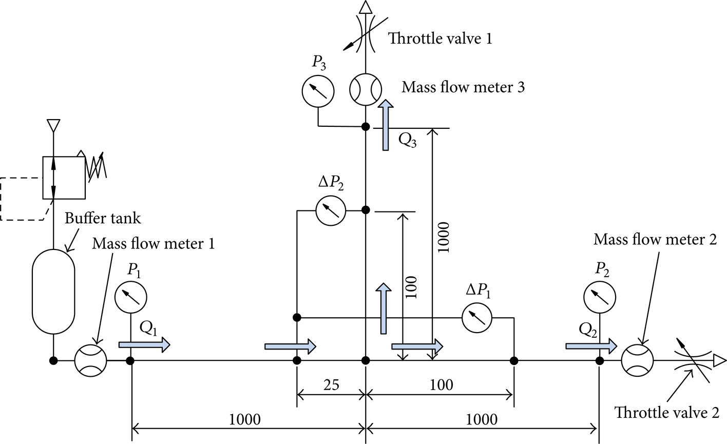
Experimental rig for static characteristic measurements in flow pattern A.

Figure 4:

Experimental rig for static characteristic measurements in flow pattern B.

The pressure sensors for P₁, P₂, and P₃ are a metal diaphragm type (“AP-13” from the KEYENCE Corp., Japan). The differential pressure sensors for ΔP₁ and ΔP₂ are also metal diaphragm type (“KL17” from the Nagano Keiki Inc., Japan). Mass flow meters are installed; however, their indication is volumetric flow rate at the ISO standard state (ISO 6358, temperature 293.15 K with pressure 100 kPa). The mass flow meters installed in the test rigs are laminar type flow meters, of which structure and characteristics are precisely described in [16].

2.2. Experimental Results

Figure 5 illustrates definitions of variables and related nomenclatures. Throughout the experiments, the upstream flow rate Q₁ is kept constant. The flow rates Q₂ and Q₃ are adjusted using throttle valves placed in the downstream of the flow meters in Figures 3 and 4.

Figure 5:

Notation used for the flow parameters in both flow patterns.

The loss coefficient is calculated using the following energy equations and measured flow rates and pressures. The flow directions from point 1 to point 2 and point 3 in patterns A and B are illustrated in Figures 5(a) and 5(b).

The energy conservation from point 1 to point 2 is expressed by

$P_{\mathrm{1}}+\frac{{\rho u}_1^2}{\mathrm{2}}=P_{\mathrm{2}}+\frac{{\rho u}_2^2}{\mathrm{2}}+\left({\lambda }_{\mathrm{1}}\frac{L_{\mathrm{1}}}{d_{\mathrm{1}}}+{\xi }_{\mathrm{12}}\right)\frac{{\rho u}_1^2}{\mathrm{2}}\mathrm{\hspace{0.17em}\hspace{0.17em}}+{\lambda }_{\mathrm{2}}\frac{L_{\mathrm{2}}}{d_{\mathrm{2}}}\frac{{\rho u}_2^2}{\mathrm{2}}.$

(1)

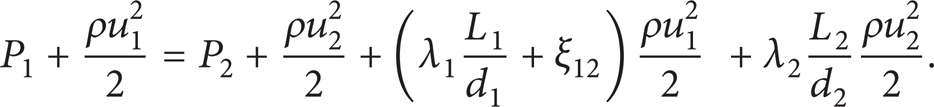
The energy conservation from point 1 to point 3 is expressed by

$P_{\mathrm{1}}+\frac{{\rho u}_1^2}{\mathrm{2}}=P_{\mathrm{3}}+\frac{{\rho u}_3^2}{\mathrm{2}}+\left({\lambda }_{\mathrm{1}}\frac{L_{\mathrm{1}}}{d_{\mathrm{1}}}+{\xi }_{\mathrm{13}}\right)\frac{{\rho u}_1^2}{\mathrm{2}}+{\lambda }_{\mathrm{3}}\frac{L_{\mathrm{3}}}{d_{\mathrm{3}}}\frac{{\rho u}_3^2}{\mathrm{2}}.$

(2)

The flow velocities shawn in these equations are calculated using the following formula:

$u_i=\frac{({\rho }_a{Q}_i/{\rho }_i)}{A}.$

(3)

The absolute pressure at the joint is about 600 kPa; however, the magnitude of the differential pressure is level of 100 Pa. While density of air is proportional to its absolute pressure, the change of the density at any point near the joint can be neglected. Hence, we can assume

${\rho }_{\mathrm{1}}={\rho }_{\mathrm{2}}={\rho }_{\mathrm{3}}=\rho .$

(4)

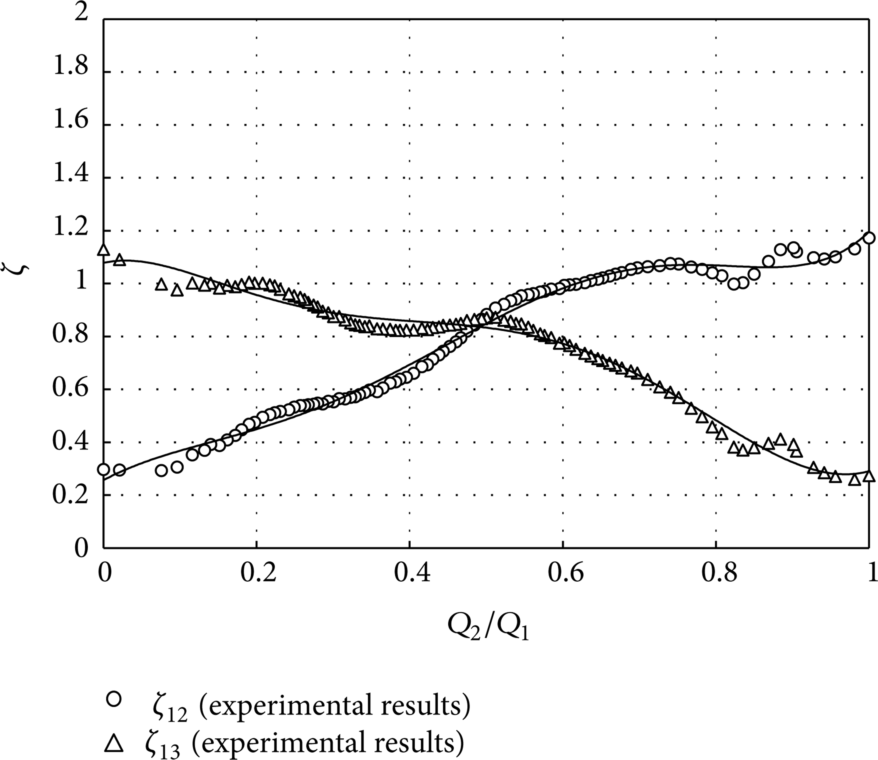
The loss coefficients of a T-joint change with the flow ratios Q₂/Q₁ and Q₃/Q₁. Figure 6 shows the static characteristic test results for pattern A, and Figure 7 shows those for pattern B. The solid lines in these figures are fit curves for the loss coefficients obtained from the experimental points in each graph. The fit curves are obtained using the least squares technique and expressed by the following polynomials of the ratio of flow rates:

${\xi }_{\mathrm{1}j}={\sum }_{n=\mathrm{0}}^{\mathrm{6}}{A}_n{q}^n,\hspace{1em}q=\frac{Q_{\mathrm{2}}}{Q_{\mathrm{1}}}.$

(5)

Figure 6:

Loss coefficients for the tee branch pipe in flow pattern A.

Figure 7:

Loss coefficients for the tee branch pipe in flow pattern B.

For pattern A, the curves in Figure 8 are fourth-order polynomials; for pattern B, the curves in Figure 9 are sixth-order polynomials. In these equations, subscripts 1j = 12 or 13 and the values of the coefficients of polynomials are shown in Table 1. The level of fit error is less than 0.3% for pattern A and 2.2% for pattern B.

Table 1:

Coefficients of polynomial fit for loss coefficients ζ_1j.

Pattern	j	A 0	A 1	A 2	A 3	A 4	A 5	A 6
A	2	0.3593	−0.6529	−0.2008	0.5926	0.1068	0	0
	3	1.0379	−0.5263	0.2735	1.7097	−0.9126	0	0
B	2	0.2567	1.5448	−6.088	19.431	16.816	−5.186	8.054
	3	0.2910	−0.8093	14.470	−32.43	20.117	8.600	−9.161

Figure 8:

Discretized blocks of pipe model.

Figure 9:

Model of the T-joint for simulation.

The static characteristic test results for pattern A shown in Figure 6 indicate that the loss coefficient ξ₁₃ in the right-angled direction is large compared with that in the straight direction. This result shows that the loss in the flow in the right-angled direction is larger than that in the flow in the straight direction. The loss coefficients shown in Figure 6 have almost the same form as the curves reported in the literature, for example, [7].

Intuitively, the loss coefficients ξ₁₂ and ξ₁₃ for pattern B will be symmetric with respect to q = 0.5. However, the measured two curves for pattern B shown in Figure 7 are not symmetric with each other. Moreover, the curves for pattern B are not so smooth as curves for pattern A. The cause of the complexity of the curves and deviation from symmetricity is supposed to be a result of complex, and sometimes irregular, eddy formation near the joint. Eddies near a T-joint of pattern B were reported by Ito et al. [8], in which they visualized the flow of water.

3. Basic Equations and Difference Equations for Simulation

In this section, an original simulation program is developed for effective and convenient study of branch pipes. One-dimensional model of fluid flow in pipes is assumed. The basic equations of one-dimensional unsteady flow in a uniform straight pipe are as follows.

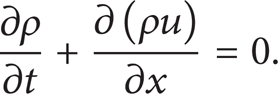
Equation of motion:

$\frac{\partial u}{\partial t}+u\frac{\partial u}{\partial x}=-\frac{\mathrm{1}}{\rho }\frac{\partial P}{\partial x}-\frac{\lambda }{\mathrm{2}d}{u}^{\mathrm{2}}.$

(6)

Equation of continuity:

$\frac{\partial \rho }{\partial t}+\frac{\partial \left(\rho u\right)}{\partial x}=\mathrm{0}.$

(7)

Equation of energy conservation:

$\frac{\partial }{\partial t}\left[\rho A\left(e+\frac{u^{\mathrm{2}}}{\mathrm{2}}\right)\right]\hspace{0.17em}+\frac{\partial }{\partial x}\left[\rho uA\left(e+\frac{u^{\mathrm{2}}}{\mathrm{2}}+\frac{P}{\rho }\right)\right]-\pi dh\left(\theta -{\theta }_a\right)=\mathrm{0}.$

(8)

Equation of state:

$P=\rho R\theta .$

(9)

Boundary conditions for the above system of equations are determined by the pipe end conditions and the mass and energy conservation at the T-joint. The boundary conditions are summarized as follows.

At the upstream end of the supply pipe:

$P=P_{\mathrm{1}}=\text{const}.\hspace{1em}\hspace{1em}\mathrm{\hspace{0.17em}\hspace{0.17em}}T=T_{\mathrm{1}}=\text{const}.$

(10)

At the downstream end of the branched pipe:

$f_{\mathrm{2}}(P_{\mathrm{2}},Q_{\mathrm{2}})=\mathrm{0},\hspace{1em}\hspace{1em}{f}_{\mathrm{3}}(P_{\mathrm{3}},Q_{\mathrm{3}})=\mathrm{0}.$

(11)

The functional relationships f₁ and f₂ are determined by throttles mounted at the pipe ends. At the T-joint, the mass conservation law is expressed by the following volumetric flow rates relation since the mass flow rate is converted to the volume flow rate using the industrial standard condition (P = 100 kPa (abs), with θ = 293.15 K):

$Q_{\mathrm{1}}=Q_{\mathrm{2}}+Q_{\mathrm{3}}.$

(12)

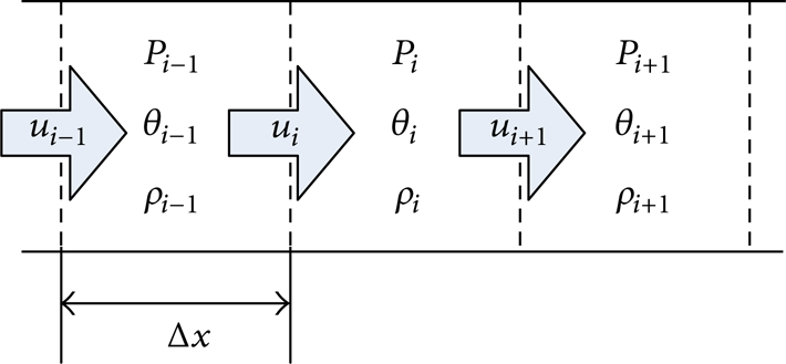
For the simulation, a straight pipe is divided into short blocks of length Δx. Time variation of the variables will be calculated with time step of Δt. The condition for convergence for hyperbolic partial differential equations [17] and reliability of calculation must be considered throughout parameter settings. A straight pipe is discretized as shown in Figure 8. The subscript of the variables in Figure 8 indicates block number.

For the simulation of unsteady flow, numbering for time step is also necessary. The second subscript is added to each variable after the block number. The first subscript in the variables in the following difference equations is the block number shown in Figure 8. The second subscript indicates the time-step number; for example, u_{i, j} means velocity at the entrance of ith block at jth time step. The upwind difference scheme is used for calculating the convection terms.

3.1. Difference Equations for Velocity

According to (6) and Figure 8, the flow velocity in ith block at jth time step can be expressed by

$\begin{array}{c}{u}_{i,j+\mathrm{1}}=u_{i,j}-\frac{\mathrm{\Delta }t}{\mathrm{\Delta }x}{u}_{\text{conv}}-\frac{\mathrm{1}}{\stackrel{-}{\rho }}\frac{\mathrm{\Delta }t}{\mathrm{\Delta }x}\left(P_{i,j}-P_{i-\mathrm{1},j}\right)-\frac{\lambda \mathrm{\Delta }t}{\mathrm{2}D}\left|u_{i,j}\right|u_{i,j},\\ u_{\text{conv}}=\frac{u_{i,j}+\left|u_{i,j}\right|}{\mathrm{2}}\left(u_{i,j}-u_{i-\mathrm{1},j}\right)-\frac{u_{i,j}-\left|u_{i,j}\right|}{\mathrm{2}}\left(u_{i+\mathrm{1},j}-u_{i,j}\right),\\ \stackrel{-}{\rho }=\frac{\left({\rho }_{i-\mathrm{1},j}+{\rho }_{i,j}\right)}{\mathrm{2}}.\end{array}$

(13)

The boundary conditions for the equation of motion are as follows.

Figure 9 shows the relationships at the joint. The algebraic expression with respect to the velocity is

$u_{n+\mathrm{1},j}=u_{a\mathrm{1},j}+u_{b\mathrm{1},j},$

(14)

and the density is

${\rho }_{n+\mathrm{1},j}=\frac{{\rho }_{a\mathrm{1},j}+{\rho }_{b\mathrm{1},j}}{\mathrm{2}}.$

(15)

The flow velocity in the a₁ block (inlet of the first branched pipe) is expressed by

$\begin{array}{c}{u}_{a\mathrm{1},j+\mathrm{1}}=u_{a\mathrm{1},j}-\frac{\mathrm{\Delta }t}{\mathrm{\Delta }x}{u}_{\text{conv}}-\frac{\mathrm{1}}{\stackrel{-}{\rho }}\frac{\mathrm{\Delta }t}{\mathrm{\Delta }x}\left(P_{a\mathrm{1},j}-P_{a\mathrm{0},j}\right)-\frac{\lambda \mathrm{\Delta }t}{\mathrm{2}D}\left|u_{a\mathrm{1},j}\right|u_{a\mathrm{1},j}-\frac{{\xi }_a\mathrm{\Delta }t}{\mathrm{2}\mathrm{\Delta }x}\frac{{\rho }_{m,j}}{{\rho }_{a\mathrm{1},j}}\left|u_{a\mathrm{0},j}\right|u_{a\mathrm{0},j},\\ u_{\text{conv}}=\frac{u_{a\mathrm{0},j}+u_{a\mathrm{1},j}}{\mathrm{2}}\left(u_{a\mathrm{1},j}-u_{a\mathrm{0},j}\right)=\frac{\mathrm{1}}{\mathrm{2}}\left(u_{a\mathrm{1},j}^{\mathrm{2}}-u_{a\mathrm{0},j}^{\mathrm{2}}\right),\\ u_{a\mathrm{0},j}=u_{n,j}.\end{array}$

(16)

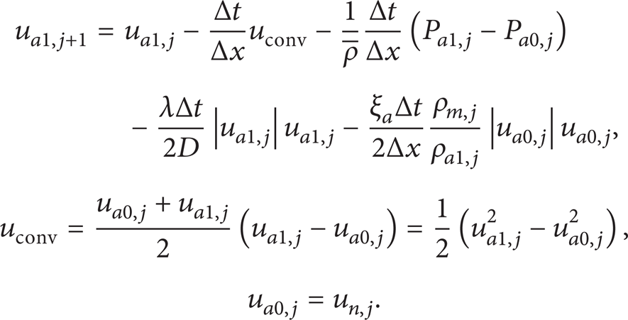
The flow velocity in the b₁ block (inlet of the second branched pipe) is obtained replacing a with b in the above three equations.

3.2. Difference Equations for Density

The density shown in the above equations must be given to satisfy the mass conservation law, (7). According tothe ith block in Figure 8 and applying the upwind difference scheme for the convection term, the difference equation of density in the ith block becomes

$\begin{array}{c}{\rho }_{i,j+\mathrm{1}}={\rho }_{i,j}-\frac{\mathrm{\Delta }t}{\mathrm{\Delta }x}{\rho }_{i,j}\left(u_{i+\mathrm{1},j}-u_{i,j}\right)-\frac{\mathrm{\Delta }t}{\mathrm{\Delta }x}{\rho }_{\text{conv}},\\ {\rho }_{\text{conv}}=\frac{{\stackrel{-}{u}}_{i,j}+\left|{\stackrel{-}{u}}_{i,j}\right|}{\mathrm{2}}\left({\rho }_{i,j}-{\rho }_{i-\mathrm{1},j}\right)+\frac{{\stackrel{-}{u}}_{i,j}-\left|{\stackrel{-}{u}}_{i,j}\right|}{\mathrm{2}}\left({\rho }_{i+\mathrm{1},j}-{\rho }_{i,j}\right).\end{array}$

(17)

The velocity with over bar in the above is

${\stackrel{-}{u}}_{i,j}=\frac{u_{i,j}+u_{i+\mathrm{1},j}}{\mathrm{2}}.$

(18)

The boundary condition at the joint with respect to the density is

$\begin{array}{c}{\rho }_{\text{conv}}=\frac{{\stackrel{-}{u}}_{a\mathrm{1},j}+\left|{\stackrel{-}{u}}_{a\mathrm{1},j}\right|}{\mathrm{2}}\left({\rho }_{a\mathrm{1},j}-{\rho }_{a\mathrm{0},j}\right)+\frac{{\stackrel{-}{u}}_{a\mathrm{1},j}-\left|{\stackrel{-}{u}}_{a\mathrm{1},j}\right|}{\mathrm{2}}\left({\rho }_{a\mathrm{2},j}-{\rho }_{a\mathrm{1},j}\right),\\ {\rho }_{a\mathrm{0},j}={\rho }_{n,j}.\end{array}$

(19)

The boundary condition at the inlet end of the main pipe is illustrated in Figure 10; numerical values of variables are given as input at the first block. The boundary condition at the exit ends is illustrated in Figure 11. In this case, functional relationship between the pressure P _m and velocity difference (u _m – u_{m + 1}) will be given as a functional relation.

Figure 10:

Boundary condition of pipe inlet end.

Figure 11:

Boundary condition of pipe exit end.

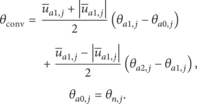
3.3. Difference Equations for Temperature

According to (8) and Figure 8, we can derive the following difference equation for temperature change in intermediate blocks of pipe model:

$\begin{array}{c}{\theta }_{i,j+\mathrm{1}}={\theta }_{i,j}-\mathrm{\Delta }t\frac{\mathrm{4}h\left({\theta }_{i,j}-{\theta }_a\right)}{{\rho }_{i,j}{C}_{V}D}-\frac{\mathrm{\Delta }t}{\mathrm{\Delta }x}{\theta }_{\text{conv}}-\frac{\mathrm{\Delta }t}{\mathrm{\Delta }x}\frac{R{\theta }_{i,j}}{C_V}\left(u_{i+\mathrm{1},j}-u_{i,j}\right)+\frac{\lambda \mathrm{\Delta }t}{\mathrm{2}{C}_{V}D}\left|{\stackrel{-}{u}}_{i,j}\right|{\stackrel{-}{u}}_{i,j}^{\mathrm{2}},\\ {\theta }_{\text{conv}}=\frac{{\stackrel{-}{u}}_{i,j}+\left|{\stackrel{-}{u}}_{i,j}\right|}{\mathrm{2}}\left({\theta }_{i,j}-{\theta }_{i-\mathrm{1},j}\right)+\frac{{\stackrel{-}{u}}_{i,j}-\left|{\stackrel{-}{u}}_{i,j}\right|}{\mathrm{2}}\left({\theta }_{i+\mathrm{1},j}-{\theta }_{i,j}\right),\\ {\stackrel{-}{u}}_{i,j}=\frac{u_{i,j}+u_{i+\mathrm{1},j}}{\mathrm{2}}.\end{array}$

(20)

The boundary condition for the temperature at the T-joint is

$\begin{array}{c}{\theta }_{\text{conv}}=\frac{{\stackrel{-}{u}}_{a\mathrm{1},j}+\left|{\stackrel{-}{u}}_{a\mathrm{1},j}\right|}{\mathrm{2}}\left({\theta }_{a\mathrm{1},j}-{\theta }_{a\mathrm{0},j}\right)+\frac{{\stackrel{-}{u}}_{a\mathrm{1},j}-\left|{\stackrel{-}{u}}_{a\mathrm{1},j}\right|}{\mathrm{2}}\left({\theta }_{a\mathrm{2},j}-{\theta }_{a\mathrm{1},j}\right),\\ {\theta }_{a\mathrm{0},j}={\theta }_{n,j}.\end{array}$

(21)

3.4. Difference Equation for Pressure

Pressure at any block is estimated using the equation of state, (9),

$P_{i,j}={\rho }_{i,j}R{\theta }_{i,j}.$

(22)

All these discretized equations are solved simultaneously at each time step. In these equations, ξ _a , ξ _b , λ, and h are given as input variable to the simulation program. The loss coefficient obtained in Section 3 is used as ξ _a = ξ₁₂ and ξ _b = ξ₁₃.

4. Experiment of Dynamic Characteristics

4.1. Experimental Setups for Dynamic Characteristic Measurements

The experimental rigs for the static characteristic measurement, which are explained in Section 2, are arranged for measurement of dynamic characteristics. Figures 12 and 13 show the rigs for the dynamic characteristic measurement for the flow patterns A and B, respectively. For pattern A, the throttle valve 2 in the downstream of the straight pipe is replaced with a servo valve. Similarly, for pattern B, the throttle valve 2 in the downstream of the branched pipe is replaced with a servo valve. In both of them, the flow rate through the servo valve is the reference input.

Figure 12:

Experimental rig for dynamic characteristic measurements in flow pattern A.

Figure 13:

Experimental rig for dynamic characteristic measurements in flow pattern B.

The flow meters used in this study are selected to meet the requirement of fast response. The working principle of the flow meters is explained in [16]; a correct measurement of oscillatory flow of up to 10 Hz is established with the flow meters. The reference pressure for the dynamic test is set to 600 kPa (abs) at the reference point stated in Section 2.

4.2. Experimental and Simulation Results

An unsteady flow was generated by giving a periodic wave signal to the servo valve. The electric signal is adjusted to generate a sinusoidal wave of flow rate. The frequencies of the sine wave signal are 1 Hz and 5 Hz. The level of flow rate Q₁ is 600 L/min (ANR); amplitude is 200 L/min (ANR). The flow through the servo valve is 100 ∼ 500 L/min (ANR); the flow through the throttle valve 1 is about 300 L/min (ANR). The temperature of the air at the T-joint is 297 + – 2 K, which is nearly equal to the ISO standard condition.

Time variations of the pressures, flow rate, and pressure differences are recorded. The differential pressures between the reference point for the T-joint and the pressure tap points, which are placed 100 mm downstream from the intersection of the pipe axes, are measured and compared with the simulation results. The experimental and simulation results are shown in Figures 14 and 15.

Figure 14:

Comparison of simulation and experimental results (pattern A: 1 Hz and 5 Hz).

Figure 15:

Comparison of simulation results with experimental results (pattern B: 1 Hz and 5 Hz).

Figures 14(a) and 14(b) show differential pressure variation in pattern A for frequencies 1 and 5 Hz, respectively. When input wave frequency is 1 Hz, the simulation and experimental results coincide well; discrepancy between the simulation and experiment rather increases at frequency 5 Hz. Figures 15(a) and 15(b) show differential pressure variation in pattern B for frequencies 1 and 5 Hz, respectively. Similar to pattern A, the simulation agrees well with the experiment at 1 Hz, and the discrepancy between the simulation and the experiment increases by 5 Hz oscillation.

A significant feature of the difference between the simulation and the experiment is the existence of higher harmonics in experimentally obtained pressure curves.

5. Discussions

The static characteristics experiment in this study was carried out to obtain the loss coefficient necessary for simulation of pressure change in oscillatory flow. Its results were not simple as expected from the literature. Therefore, we explained the result of the static loss coefficient rather precisely.

The pipe Reynolds number in the static experiment lies between 18,000 and 53,000. In this range, the change of loss coefficient with the Reynolds number is very small. While the Mach number varies along the pipes, it is smaller than 0.1 throughout the experiment. Hence, the influence of the Mach number is also negligible, and the flow can be assumed to be incompressible. In this state, each loss coefficient at the T-joint becomes single function of the ratio of the flow rates. The obtained experimental results for the static characteristics are compared with the data in the literature, for example, [7]. The data of pattern A agree with [7]. However, no equivalent data for pattern B was found. In this experiment, diameter of the main and the branched pipes is the same; data in the literature shows diameter ratio of smaller than 1. Under this circumstance, the obtained data for pattern B was rather curious; the two loss coefficients for geometrically equivalent branches did not show expected symmetry with respect to flow ratio q = 0.5. Naturally, the conclusion will become different if smaller Reynolds number is selected; however, it will be a subject of another study.

The dynamic characteristics are not simply dependent on the flow ratio. It is influenced by additional parameters that do not appear in the steady state. For example, pressure wave reflections from pipe ends take a part of the pressure at the T-joint in dynamics while they give no influence for static characteristics. Therefore, the influence of compressibility is not negligible in dynamic characteristics.

The simulation in Section 4 was carried out using the statically measured values of the loss coefficient. As shown in Section 4, the discrepancy of the differential pressures between simulation and the corresponding experiment for 5 Hz is greater than that of 1 Hz. This indicates frequency dependence of the loss coefficient.

The wave forms of the differential pressure for pattern A with 1 Hz are very similar to a sine wave; however, those for pattern B show rather large distortion from sine waves. This reflects the nonuniformity of loss coefficient curves in Figure 9.

There is commercial simulation software from many companies. Such software is designed to meet nonspecified customers, which is often inconvenient for a special scientific purpose. Therefore, this study built a simulation program specialized for branch pipe. The validity of the simulation model built in Section 4 is examined giving input flow of different frequencies. Results of simulation are compared with experimental results. The difference between the experiments and the simulation is by no means zero. The cause of difference can exist in the modeling error and the noise in the experimental data.

There are two major causes of modeling error: discretizing errors with respect to time and space and the one-dimensional assumption. The discretizing error became acceptable level by repeated trials of different step sizes. While the one-dimensional assumption is widely used [18–20], and its validity is proved to a certain degree, however, its definitive validation for each practical case requires experimental evidence. Therefore, comparison of simulation and experimental results is carried out in this study.

In the dynamics experiment, the sensor and amplifier output involves noises from various sources; therefore, filters are used to reject the noises. Although the use of a filter is effective for removing the noises, it also attenuates higher harmonics in a real signal. A suitable cut-off frequency is influenced by the noise that depends on experimental rigs and circumstances; therefore, careful trial-and-error process for selection of the cut-off frequency is important. After some trial of cut-off frequencies, we found that cut-off frequencies about five times as high as input frequency is near-best choice in this series of experiment. Therefore, the filter cut-off frequency is five times as high as the input sine wave frequency in the dynamics experiment.

Figures 14 and 15 shows two cycles of the signals; the good periodicity of the experimental results indicates that noises are effectively removed. Non-linearity in a system causes sometimes generation of sub-harmonics. The two figures suggest that a small component of 1/2 harmonic might exist in the experimental result although it is not appear in the simulation. Therefore, the observed sub-harmonic in the experimental result is not caused by the theoretical non-linearity, which is expressed by square of velocity in equations; it must be low frequency noise.

6. Conclusions

The pressure loss coefficients at a T-joint are measured for two patterns of flow. While the data from pattern A gave supposed values, data from pattern B did not have supposed symmetric feature.

Simulation and experimental measurement are carried out for the pressure change in a branch pipe induced by oscillatory flow at a terminal of a branch. Simulation program is made based on the one-dimensional flow model. Experiments and simulation are compared for oscillatory flow of 1 and 5 Hz; they concide well in the two patterns of branch pipe flow.