Approximate Techniques in Solving Optimal Camera Placement Problems

Abstract

While the theoretical foundation of the optimal camera placement problem has been studied for decades, its practical implementation has recently attracted significant research interest due to the increasing popularity of visual sensor networks. The most flexible formulation of finding the optimal camera placement is based on a binary integer programming (BIP) problem. Despite the flexibility, most of the resulting BIP problems are NP-hard and any such formulations of reasonable size are not amenable to exact solutions. There exists a myriad of approximate algorithms for BIP problems, but their applications, efficiency, and scalability in solving camera placement are poorly understood. Thus, we develop a comprehensive framework in comparing the merits of a wide variety of approximate algorithms in solving the optimal camera placement problems. We first present a general approach of adapting these problems into BIP formulations. Then, we demonstrate how they can be solved using different approximate algorithms including greedy heuristics, Markov-chain Monte Carlo, simulated annealing, and linear and semidefinite programming relaxations. The accuracy, efficiency, and scalability of each technique are analyzed and compared in depth. Extensive experimental results are provided to illustrate the strength and weakness of each method.

1. Introduction

Due to the significant progress in visual sensor technology, wireless communication, and pattern recognition algorithms, the deployment of wide-area visual sensor networks has become practical and cost-effective. These networks have a wide range of commercial and military applications from video surveillance to smart home and from traffic monitoring to antiterrorism. A proper placement of different visual sensors in the target environment is an important design problem as it has a direct impact on both the cost and performance of the network. The number of sensors, the dedicated communication networks, and the proper routing of power supply can contribute a significant portion of the overall construction cost. The placement of the sensors also determines the size and shape of the coverage area as well as the visual appearance of all surveillance subjects, which affect the performance of all subsequent computer vision and pattern recognition tasks.

However, even with decades of study in camera placement design, the most ambitious goal of designing a universal camera network configuration tool has not yet been achieved. The difficulties come from a variety of factors. First, cameras are vulnerable to occlusions by both static and dynamic objects. A typical wide-area indoor or outdoor environment is often characterized by complicated topologies, stringent placement constraints, and a constant flux of occupant or vehicular traffic. A decent configuration tool must take into account all these factors so as to minimize the amount of occlusion. Second, different applications impose very different performance objectives and requirements on camera networks. Simply maximizing the coverage is no longer adequate for modern applications. For example, object identification or biometric applications may require minimum object size and specific pose to ensure proper detection. Traffic measurement applications may require observation of full trajectories or proper segmentation of pedestrians. 3D reconstruction or distributed camera hand-off algorithms require multiple camera views on the same object. Resource constraints such as number of cameras, types of cameras, connectivity between neighboring cameras, power consumption, and camera movement controls are routinely used to reflect limitations in realistic deployment. A universal camera placement framework must be able to accommodate all these sometimes contradictory requirements in a single optimization framework.

Classical approaches formulate the camera placement problem as a geometry problem over the continuous space of the physical environment and camera network configuration. With the tremendous complexity in modeling camera visibility, environment topology, and the disparate application requirements mentioned above, it is difficult if not impossible to capture all aspects of the problem via any continuous-domain approach. As such, most of the camera placement researches resort to discrete approaches, where the physical environment and the camera network configuration search space are first discretized. A binary variable is defined for each point in the search place to indicate the possible presence of a camera at that location and pose. The totality of these camera variables defines the configuration of a camera network which in turn determines the visibility binary variable at each point of the physical environment. Application-specific constraints and objective functions can then be defined based on these variables to formulate a binary integer programming (BIP) optimization problem.

While the BIP formulation provides great flexibility in modeling the camera placement problem, BIP optimization problems are notorious to solve in practice. Many BIP formulations of camera placement are NP-complete, where exact solutions are too complex to obtain even for a small-size problem. As a result, a myriad of approximate algorithms have been applied in solving BIP-based camera placement problem. However, many of the proposed approaches [1–8] are customized for specific applications and a fair evaluation of different approximate algorithms on solving the general camera placement problem remains elusive.

In this paper, we present the BIP formulation for a wide variety of camera placement problems and provide a comprehensive framework to study various approximation algorithms in solving them. Specifically, we consider two general camera placement problems: the MIN formulation in which the camera resource is minimized for a target performance, and the FIX formulation in which the target performance is maximized under a resource constraint. Many other commonly used constraints in camera network design are also discussed. To solve the BIP-based camera placement problems, we have applied a spectrum of approximate algorithms from greedy, heuristics, Markov-chain Monte Carlo, simulated annealing, linear programming relaxation, and semidefinite programming relaxation. The accuracy, efficiency, and scalability of each technique are analyzed and compared in depth. Extensive experimental results are also provided to illustrate the strengths and weaknesses of each method. To the best of our knowledge, this is the first comprehensive comparison of various approximate algorithms in solving the camera placement problems. Compared with an earlier version of this work [9], we have further expanded the BIP framework to handle a richer set of objective functions and constraints and included more experimental results to compare various approximate algorithms.

The paper is organized as follows. First, we give a brief literature review in Section 2. Section 3 defines the two camera placement problems and formulates them via a BIP framework to incorporate some of the most commonly used objective functions and constraints. In Section 4, we introduce different approximate algorithms and present details on the adaptation of each algorithm in solving the BIP camera placement problems. Extensive experimental results are presented in Section 5 to compare their performances. We conclude our paper in Section 6.

2. Related Work

The problem of optimal camera placement has been studied for decades. The earliest investigation can be traced back to the “art gallery problem” in computational geometry. This problem is the theoretical study on how to place cameras in an arbitrary-shaped polygon so as to cover the entire area [10–12]. It covers a set of important topics in computational geometry including Delaunay triangulation and vertex covering. While Chvátal has shown in [13] that the upper bound of the number of cameras is $\lfloor n/\mathrm{3}\rfloor$ , determining the minimum number of cameras turns out to be a NP-complete problem [14]. While the theoretical difficulties of the camera placement problem are well understood, few solutions can be directly applied to realistic computer vision problems—the original formulation of the “art gallery” problem lacked realistic models for either the cameras or the environment under surveillance and provided few efficient computational approaches to calculate optimal placements under different scenarios. Camera placement has also been studied in the field of photogrammetry in order to obtain the most accurate 3D reconstruction of the scene. Various metrics such as visual hull [15] and viewpoint entropy [16] have been developed and optimization is realized by various types of ad-hoc searching and heuristics [17]. These techniques assume very dense placement of cameras and are not applicable to wide-area wide-baseline camera networks.

Recent widespread deployments of video camera networks, however, turned camera placement from a problem of theoretical interest into an important tool that can significantly improve the performance, coverage, and cost-effectiveness of the network. While the original “art gallery” problem was formulated in the continuous 2D or 3D spaces, the complexity of modeling visibility in continuous space increases dramatically when practical considerations such as orientation and multiple views are incorporated. Sophisticated continuous-space modeling pertinent to visual sensor networks is recently proposed in [18, 19]. The sophistication in their visibility models has greatly limited their practical usage in wide-area surveillance environments.

As such, the majority of the recent approaches consider the problem entirely in discrete domain—instead of optimizing continuous functionals using calculus of variation, discrete-domain approaches quantize the search space into finitely many candidate positions and search for the best configurations that optimize a target objective function. This strategy naturally leads to combinatorial problems with the camera, environment, and traffic models encoded in different integral constraints and objective functions. Horster and Lienhart [1] made an early effort to use generic BIP to formulate the discrete camera placement problem. Our earlier work in [20] followed a similar optimization strategy but with more sophisticated probabilistic model approach to capture the uncertainty of object orientation and mutual occlusion. Similar works can be found in [6, 8]. In Ercan's formulation the objective contains quadratic term so quadratic programming was used instead of BIP which requires all terms to be linear [8].

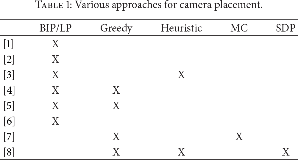
While most of the formulations result in NP-hard problems, a myriad of practical solutions including binary integer programming solvers (BIP), greedy approach, greedy heuristics, Markov-Chain Monte Carlo (MCMC), and semidefinite programming relaxations (SDP) have been proposed [1–8]. Each method has its own merits in terms of ease of formulation, computational complexity, worst or average case performances, scalability, and so forth. To further complicate matters, different researchers often tackle slightly different objective functions and design specific approximation techniques accordingly. To the rest of the vision community, it is difficult to discern the merits of different approaches and to identify the appropriate solution for a specific placement problem at hand. It is our goal to provide the pros and cons of using different approximate algorithms in solving the camera placement problem. Table 1 lists the approximate algorithms tested in this paper and their usage in existing works.

Table 1

Various approaches for camera placement.

	BIP/LP	Greedy	Heuristic	MC	SDP
[1]	X
[2]	X
[3]	X		X
[4]	X	X
[5]	X	X
[6]	X
[7]		X		X
[8]		X	X		X

3. Camera Placement in General

In this section, we define the two camera placement problems and formulate them via a BIP framework to incorporate some of the most commonly used objective functions and constraints.

3.1. BIP Formulation

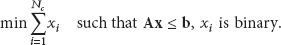
Although there is a myriad of camera placement problems in the literature, the fundamental objectives of these problems almost always fall into two broad categories which we refer to as the MIN and FIX problems.

• (1)

The goal of the MIN problems is to minimize the number of cameras such that the target coverage p can be achieved subject to other constraints.

(2)

The goal of the FIX problems is to maximize the coverage subject to a fixed number of cameras m and other application specific constraints.

Both problems can be tackled in the following fashion. First, the space of possible camera configurations, including locations, yaw, pitch angles, and camera types, can be converted into discrete points by either random [1] or uniform sampling [6, 20]. The target space of the camera network can also be discretized into a finite space, which can be the 2D [7] or 3D [18], object positions, object orientations [21], motion paths [18] or even a combination of all the above spaces.

We denote the discretized camera space as $\{{{\rm Y}}_i:i=\mathrm{1},\dots ,N_c\}$ and the target space as $\{{\mathrm{\Lambda }}_j:j=\mathrm{1,2},\dots ,N_p\}$ . We then define two sets of binary variables $\{b_i:i=\mathrm{1},\dots ,N_c\}$ and $\{x_j:j=\mathrm{1},\dots ,N_p\}$ on the two spaces, respectively. Each $b_i=\mathrm{1}$ for $i=\mathrm{1},\dots ,N_c$ indicates that a camera is placed or selected at ${{\rm Y}}_i$ . A camera placement plan is represented by a particular selection of these $b_i$ variables and the goal of the placement problem is to find a placement plan that optimizes the objective functions and satisfies all given constraints. $x_j$ for $j=\mathrm{1},\dots ,N_p$ becomes 1 if an object placed at ${\mathrm{\Lambda }}_j$ can be observed under the selected camera plan. Obviously, each $x_j$ is determined by the $b_i$ variables, and their relationships are using manifested constraints as we will illustrate in Section 3.2. Using these variables, the MIN and FIX formulations can be formulated as follows:

$$\begin{array}{l}\text{MIN}:\hspace{1em}\text{minimize}{\displaystyle \sum }_{i=\mathrm{1}}^{N_c}‍b_i\\ \hspace{1em}\hspace{1em}\hspace{1em}\hspace{0.17em}\text{given}\mathrm{\hspace{0.17em}\hspace{0.17em}}f(x_{\mathrm{1}},\dots x_{N_p})\ge p,\hspace{1em}{x}_j,b_i\mathrm{\hspace{0.17em}\hspace{0.17em}}\text{are binary},\end{array}$$

(1)

$$\begin{array}{l}\mathrm{\hspace{0.17em}\hspace{0.17em}}\text{FIX}:\hspace{1em}\mathrm{\hspace{0.17em}\hspace{0.17em}}\text{maximize}\mathrm{\hspace{0.17em}\hspace{0.17em}}f(x_{\mathrm{1}},\dots x_{N_p})\\ \hspace{1em}\hspace{1em}\hspace{1em}\hspace{0.17em}\text{given}\mathrm{\hspace{0.17em}\hspace{0.17em}}\mathrm{\hspace{0.17em}\hspace{0.17em}}{\displaystyle \sum }_{i=\mathrm{1}}^{N_c}‍b_i\le m\text{,}\mathrm{\hspace{0.17em}\hspace{0.17em}}\hspace{1em}{x}_j,b_i\mathrm{\hspace{0.17em}\hspace{0.17em}}\text{are binary,}\mathrm{\hspace{0.17em}\hspace{0.17em}}\end{array}$$

(2)

where $f(x_{\mathrm{1}},\dots ,x_{N_p})$ is an application-specific real-valued function that measures the coverage of the network. A simple but powerful example of $f(x_{\mathrm{1}},\dots ,x_{N_p})$ would be $(\mathrm{1}/N_p){\sum }_{j=\mathrm{1}}^{N_p}‍{\rho }_j{x}_j$ , where ${\rho }_j\in [\mathrm{0,1}]$ are known weights derived from the particular application to represent the importance of the area around the discretized location. For instance, in [22], a random walker model is used to calculate the weights to embody the likelihood of moving object to occur in a particular region. In order to provide a baseline for comparison without losing generality, we adopt this model in this paper and set ${\rho }_j=\mathrm{1}$ for simplicity, but a more sophisticated metric that considers other factors can also be used. Application-specific constraints should also be added to represent the internal relationship between the two sets of variables.

We assume that the coverage function and all constraints are linear in $x_j$ 's and $b_i$ 's. This assumption is not overly restrictive as there are general strategies to convert nonlinear constraints into linear ones [23]. Here we provide a few examples which include common techniques to linearize the nonlinear requirements that arise in camera planning.

3.2. Common Constraints Used in Camera Planning

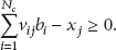
3.2.1. Visibility Constraint

To determine if a particular target grid point ${\mathrm{\Lambda }}_j$ by a camera at $b_i$ is determined by the target application and can be complicated affairs, it can depend on, but certainly not limited to, all optical properties of camera, environmental occlusion, mutual occlusion from other objects, and self-occlusion. However, as shown in [5], such complexity can be hidden via a precomputed visibility matrix V where $v_{ij}=\mathrm{1}$ implies that the target position ${\mathrm{\Lambda }}_j$ is visible at the camera at ${{\rm Y}}_i$ . With the visibility matrix, we can define a set of visibility binary variables $x_j$ 's which indicate whether an object at particular target grid point ${\mathrm{\Lambda }}_j$ is visible to at least one selected camera. The relationship between V, $b_i$ 's, and $x_j$ 's can be expressed via a set of pairs of visibility constraints as follows. For each target grid point ${\mathrm{\Lambda }}_j$ for $j=\mathrm{1,2},\dots ,N_p$ , we have

$$\begin{array}{cc}& {\displaystyle \sum }_{i=\mathrm{1}}^{N_c}‍v_{ij}{b}_i-N_c{x}_j\le \mathrm{0},\end{array}$$

(3)

$$\begin{array}{cc}& {\displaystyle \sum }_{i=\mathrm{1}}^{N_c}‍v_{ij}{b}_i-x_j\ge \mathrm{0}.\end{array}$$

(4)

These two constraints define the binary variable $x_j$ : for $x_j=\mathrm{1}$ , Inequality (3) is obviously true while Inequality (4) ensures that at least one camera that can see ${\mathrm{\Lambda }}_j$ is selected in the placement plan. For $x_j$ , the situation is reverse and Inequality (3) forces that none of the cameras that can capture ${\mathrm{\Lambda }}_j$ is selected.

In this example, we only select the first camera, so $b_{\mathrm{1}}=\mathrm{1}$ , $b_{\mathrm{2}}=b_{\mathrm{3}}=\mathrm{0}$ , and

$$\begin{array}{cc}& V=\left(\begin{array}{ccc}\mathrm{1}& \mathrm{0}& \mathrm{0}\\ \mathrm{0}& \mathrm{1}& \mathrm{0}\\ \mathrm{0}& \mathrm{0}& \mathrm{1}\end{array}\right).\end{array}$$

(5)

For ${\mathrm{\Lambda }}_{\mathrm{1}}$ , we have ${\sum }_{i=\mathrm{1}}^{N_c}‍v_{ij}{b}_i=v_{\mathrm{11}}{b}_{\mathrm{1}}+v_{\mathrm{21}}{b}_{\mathrm{2}}+v_{\mathrm{31}}{b}_{\mathrm{3}}=\mathrm{1}$ , so (3) becomes

$$\begin{array}{cc}& \mathrm{1}-\mathrm{3}{x}_{\mathrm{1}}\le \mathrm{0}\end{array}$$

(6)

and (4) becomes

$$\begin{array}{cc}& \mathrm{1}-x_{\mathrm{1}}\ge \mathrm{0}.\end{array}$$

(7)

Solving the equations above, we have $\mathrm{1}/\mathrm{3}\le x_{\mathrm{1}}\le \mathrm{1}$ , and since $x_i$ is binary so we have $x_{\mathrm{1}}=\mathrm{1}$ .

For ${\mathrm{\Lambda }}_{\mathrm{2}}$ , we have ${\sum }_{i=\mathrm{1}}^{N_c}‍v_{ij}{b}_i=v_{\mathrm{12}}{b}_{\mathrm{1}}+v_{\mathrm{22}}{b}_{\mathrm{2}}+v_{\mathrm{32}}{b}_{\mathrm{3}}=\mathrm{0}$ , so (3) becomes

$$\begin{array}{cc}& \mathrm{0}-\mathrm{3}{x}_{\mathrm{2}}\le \mathrm{0}\end{array}$$

(8)

and (4) becomes

$$\begin{array}{cc}& \mathrm{0}-x_{\mathrm{2}}\ge \mathrm{0}.\end{array}$$

(9)

Solving the equations above, we have $\mathrm{0}\le x_{\mathrm{2}}\le \mathrm{0}$ so we have $x_{\mathrm{2}}=\mathrm{0}$ .

Similarly, for ${\mathrm{\Lambda }}_{\mathrm{3}}$ . we have $x_{\mathrm{3}}=\mathrm{0}$ , which conforms to our application scenario that if we only select camera 1, then only target 1 is visible.

It is a straightforward matter to extend the basic case of visibility to multiple coverage requirement in which an object is considered visible when it is seen by at least $k>\mathrm{1}$ cameras. Multiple camera coverage constraint is important to computer vision applications where reconstruction algorithms are applied to recover missing information due to occlusion and projective distortion. This requirement can be imposed by a small modification on the thresholds as follows:

$$\begin{array}{cc}& {\displaystyle \sum }_{i=\mathrm{1}}^{N_c}‍v_{ij}{b}_i-\left(N_c-k+\mathrm{1}\right)x_j\le k-\mathrm{1},\\ {\displaystyle \sum }_{i=\mathrm{1}}^{N_c}‍v_{ij}{b}_i-k{x}_j\ge \mathrm{0}.\end{array}$$

(10)

3.2.2. Connectivity

Connectivity requirements impose certain communication limitations on how the camera nodes can communicate with each other. It is typical requirement in wireless camera network where only nearby camera nodes can communicate between each other due to the power constraints. To model such a neighborhood relationship, we introduce an adjacency matrix A with each entry $a_{ij}=\mathrm{1}$ if cameras at i and j are connected. We also define a binary variable $y^{ij}=\mathrm{1}$ if there is a communication flow between camera ${{\rm Y}}_i$ to ${{\rm Y}}_j$ whenever both cameras are selection. Mathematically, it is defined as follows:

$$\begin{array}{cc}& y^{ij}\le \frac{a_{ij}}{\mathrm{2}}\left(b_i+b_j\right).\end{array}$$

(11)

The connectivity is ensured by requiring that every selected camera has at least one flow so that the observed information can be routed out:

$$\begin{array}{cc}& b_i\le {\displaystyle \sum }_j‍y^{ij}.\end{array}$$

(12)

A more complicated example considering communication capacity and different type of sensors can be found in [24].

3.2.3. Localization Error

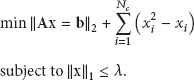
Localization error indicates the possible error in estimating the location of an object. This function is not isotropic due to the nature of perspective projection. In [8], the authors model the 2D localization error of tracking a single nonoccluded object, given its first and second order statistics, as the minimum mean-square error of the linear estimate based on the perspectively distorted images at the camera. In the 2D case, this location error is a function of the yaw angle 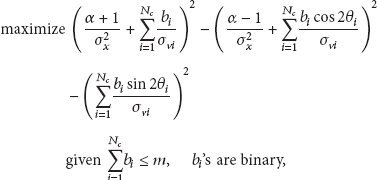${\theta }_i$ of each camera i. As such, they formulate the camera placement problem as follows:

$$\begin{array}{l}\mathrm{\hspace{0.17em}\hspace{0.17em}}\text{maximize}\mathrm{\hspace{0.17em}\hspace{0.17em}}{\left(\frac{\alpha +\mathrm{1}}{{\sigma }_x^{\mathrm{2}}}+{\displaystyle \sum }_{i=\mathrm{1}}^{N_c}‍\frac{b_i}{{\sigma }_{vi}}\right)}^{\mathrm{2}}-{\left(\frac{\alpha -\mathrm{1}}{{\sigma }_x^{\mathrm{2}}}+{\displaystyle \sum }_{i=\mathrm{1}}^{N_c}‍\frac{b_i\cos \mathrm{2}{\theta }_i}{{\sigma }_{vi}}\right)}^{\mathrm{2}}\\ \hspace{1em}\hspace{1em}\hspace{1em}\hspace{1em}-{\left({\displaystyle \sum }_{i=\mathrm{1}}^{N_c}‍\frac{b_i\sin \mathrm{2}{\theta }_i}{{\sigma }_{vi}}\right)}^{\mathrm{2}}\\ \hspace{1em}\hspace{1em}\hspace{1em}\hspace{1em}\text{given}\mathrm{\hspace{0.17em}\hspace{0.17em}}{\displaystyle \sum }_{i=\mathrm{1}}^{N_c}‍b_i\le m\text{,}\mathrm{\hspace{0.17em}\hspace{0.17em}}\hspace{1em}{b}_i\text{'s}\mathrm{\hspace{0.17em}\hspace{0.17em}}\text{are binary,}\mathrm{\hspace{0.17em}\hspace{0.17em}}\end{array}$$

(13)

where ${\sigma }_v$ is the measurement noise variance, ${\sigma }_x$ is the localization noise prior, and α is a parameter to indicate the asymmetry of prior noise in the two principal axes. Note that ${\theta }_i$ is not a variable here but rather the specific yaw angle specified by the specific camera pose assigned to the variable $b_i$ . The authors argued that as this objective function is quadratic, it is not amenable to linear techniques and they used SDP to solve the optimization problem. Nevertheless, using additional variables, it can be shown that this formulation can be easily linearized into a linear BIP and can thus be absorbed into our proposed framework.

The linearization is shown as below. First, the objective function can be expanded into the following form:

$$\begin{array}{l}\frac{\mathrm{4}\alpha }{{\sigma }_x^{\mathrm{4}}}+\frac{\mathrm{2}\left(\alpha +\mathrm{1}\right)}{{\sigma }_x^{\mathrm{2}}}{\displaystyle \sum }_i‍\frac{b_i}{{\sigma }_{v_i}^{\mathrm{2}}}+\frac{\mathrm{2}\left(\alpha -\mathrm{1}\right)}{{\sigma }_x^{\mathrm{2}}}{\displaystyle \sum }_i‍\frac{\cos \mathrm{2}{\theta }_i{b}_i}{{\sigma }_{v_i}^{\mathrm{2}}}\\ \hspace{1em}+\mathrm{2}{\displaystyle \sum }_i‍{\displaystyle \sum }_j‍\frac{\mathrm{1}-\cos \mathrm{2}{\theta }_i\cos \mathrm{2}{\theta }_j-\sin \mathrm{2}{\theta }_i\sin \mathrm{2}{\theta }_j}{{\sigma }_{v_i}^{\mathrm{2}}{\sigma }_{v_j}^{\mathrm{2}}}{b}_i{b}_j,\end{array}$$

(14)

where the only variables are $b_i$ 's. Though the expression is not linear due to the presence of the cross term $b_i{b}_j$ , we can linearize it by replacing $b_i{b}_j$ with new binary variables $y_{ij}$ and adding three sets of linear constraints as follows:

$$\begin{array}{cc}& -b_i+y_{ij}\le \mathrm{0},\\ -b_j+y_{ij}\le \mathrm{0},\\ b_i+b_j-y_{ij}\le \mathrm{1}.\end{array}$$

(15)

3.2.4. Tracking Performance

Tracking is the process of locating moving objects through a camera network in a continuous fashion. The crucial element for tracking is occlusion handling. In the sense of camera placement or selection, it means the continuous time interval when the object is not observed should be minimized. To incorporate such a constraint, we need to introduce additional path variable ${\mathrm{\Psi }}_j$ for each sample path of interest. Continuous tracking of the path ${\mathrm{\Psi }}_j$ can be represented by a linear constraints as follows:

$$\begin{array}{cc}& {\displaystyle \sum }_{i\in {\mathrm{\Psi }}_j}‍x_i\ge \eta \left|{\mathrm{\Psi }}_j\right|,\end{array}$$

(16)

where $|\mathrm{\Psi }|$ is the length of the path in terms of the environment sample points and η is the minimum percentage of the entire path that must be visible.

3.2.5. Partial Coverage

In some computer vision applications, a simple binary visibility metric is inadequate. For instance, in facial recognition systems, face image with a lower resolution has a higher probability to produce erroneous matching than a high resolution image. As such, it requires an objective function that can gracefully degrade from a fully visible state to a complete miss. A fuzzy model has been introduced in [25] for this purpose, and it can be easily incorporated into our BIP model. Let 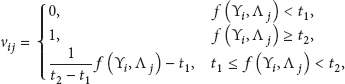$f({{\rm Y}}_i,{\mathrm{\Lambda }}_j)$ be a real-valued function that measures the continuous image quality of an object ${\mathrm{\Lambda }}_j$ from a camera at ${{\rm Y}}_i$ . All we need is to redefine $v_{ij}$ in (3) as follows:

$$\begin{array}{cc}& v_{ij}=\{\begin{array}{cc}\mathrm{0},\hfill & f\left({{\rm Y}}_i,{\mathrm{\Lambda }}_j\right)<t_{\mathrm{1}},\hfill \\ \mathrm{1},\hfill & f\left({{\rm Y}}_i,{\mathrm{\Lambda }}_j\right)\ge t_{\mathrm{2}},\hfill \\ \frac{\mathrm{1}}{t_{\mathrm{2}}-t_{\mathrm{1}}}f\left({{\rm Y}}_i,{\mathrm{\Lambda }}_j\right)-t_{\mathrm{1}},\hfill & t_{\mathrm{1}}\le f\left({{\rm Y}}_i,{\mathrm{\Lambda }}_j\right)<t_{\mathrm{2}},\hfill \end{array}\end{array}$$

(17)

where $t_{\mathrm{1}}$ , $t_{\mathrm{2}}$ are upper and lower threshold for a computer vision task.

3.2.6. Group Constraint

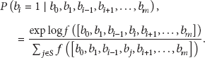
Group constraint is used to impose different requirements on a subset of the parameter space. For instance, the control of a PTZ camera can be formulated as a group constraint over binary camera variables with known position but unknown pose. Suppose the spatial positions of the cameras have already been determined and the goal is to determine the optimal pose for the visible task. At a specific camera location 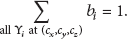$(c_x,c_y,c_z)$ in the 3D space, there is a set of camera variables $b_i$ that are associated with the different allowable pose. As a PTZ camera cannot be at two different poses simultaneously, we can use the following equality constraint to ensure this condition:

$$\begin{array}{cc}& {\displaystyle \sum }_{\mathrm{\hspace{0.17em}\hspace{0.17em}}\text{all}\hspace{0.17em}\hspace{0.17em}{{\rm Y}}_i\mathrm{\hspace{0.17em}\hspace{0.17em}}\text{at}\mathrm{\hspace{0.17em}\hspace{0.17em}}(c_x,c_y,c_z)\mathrm{\hspace{0.17em}\hspace{0.17em}}}‍b_i=\mathrm{1}.\end{array}$$

(18)

Similar constraints can be found in [26] where a set of inequalities are used to prevent multiple cameras to be placed at the same physical position.

3.2.7. Placement of Stereo Sensors

BIP can be also used to model planning of stereo sensors, in which we try to minimize the number of cameras while ensuring every target has been covered by a stereo pair. We provide an alternative BIP formulation to the ones proposed in [4]. The visibility variable 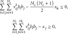$x_k$ at ${\mathrm{\Lambda }}_k$ is defined based on its visibility by stereo pairs of cameras as follows:

$$\begin{array}{cc}& {\displaystyle \sum }_{i=\mathrm{1}}^{N_c}‍{\displaystyle \sum }_{j=i+\mathrm{1}}^{N_c}‍v_{ij}^k{b}_i{b}_j-\frac{N_c\left(N_c+\mathrm{1}\right)}{\mathrm{2}}{x}_k\le \mathrm{0},\\ {\displaystyle \sum }_{i=\mathrm{1}}^{N_c}‍{\displaystyle \sum }_{j=i+\mathrm{1}}^{N_c}‍v_{ij}^k{b}_i{b}_j-x_j\ge \mathrm{0},\end{array}$$

(19)

where $v_{i,j}^k$ is the stereo visibility metric defined as follows: in [4], a target at ${\mathrm{\Lambda }}_k$ is visible by a pair of cameras at ${{\rm Y}}_i$ and ${{\rm Y}}_j$ if (1) it is within a distance range between $d_{\mathrm{1}}$ and $d_{\mathrm{2}}$ from both cameras, (2) the angle suspended at the object between the stereo pair $\angle {{\rm Y}}_i{\mathrm{\Lambda }}_k{{\rm Y}}_j$ must be narrow enough to satisfy the baseline requirement. These criteria lead to the following:

$$\begin{array}{cc}& v_{ij}^k=\{\begin{array}{cc}\mathrm{1},\hfill & \text{if}\mathrm{\hspace{0.17em}\hspace{0.17em}}{d}_{\mathrm{1}}\le d\left({{\rm Y}}_i,{\mathrm{\Lambda }}_k\right),\mathrm{\hspace{0.17em}\hspace{0.17em}}d\left({{\rm Y}}_j,{\mathrm{\Lambda }}_k\right)\le d_{\mathrm{2}},\hfill \\ \hfill & \angle {{\rm Y}}_i{\mathrm{\Lambda }}_k{{\rm Y}}_j\le \theta ,\hfill \\ \mathrm{0},\hfill & \text{otherwise,}\hfill \end{array}\end{array}$$

(20)

where $d(·,·)$ is the Euclidean distance function and $d_{\mathrm{1}}$ , $d_{\mathrm{2}}$ , θ are predetermined constants. The same method described in Section 3.2.3 can be used to make the constraint linear.

4. Approximate Solutions to BIP Camera Placement Problems

The number of variables in camera placement problems is directly proportional to the volume of the search space and is typically very large even for simple environments. Although there is optimization software capable of solving BIP problems exactly, it is in general impractical or even impossible to obtain an exact solution for any reasonable-size camera placement problem. In this section, we investigate several approximate algorithms for camera placement problems and we will show how close approximated solutions are to the exact solutions by simulations in Section 5.

4.1. Greedy Method

The greedy method is probably the most intuitive method in solving camera placement problems. The basic idea is that instead of seeking a global optimum by checking all possible configurations, we choose one camera that optimizes the objective value at each step. The advantages of the greedy algorithm include a simple implementation and tremendous efficiency—most greedy algorithms have $O(n)$ complexity instead of $O(n^k)$ by using an exhaustive search, where n is the size of the camera space. A generalized greedy algorithm for both the MIN and FIX problems is shown in Algorithm 1.

Algorithm 1: A greedy search camera placement algorithm.

Input:  Initial grid points for cameras Υ and targets Λ, feasible sets defined

    by other constraints S, the target mean visibility p, maximum

    number of cameras m, minimum camera coverage $k\ge \mathrm{1}$

Output:  Camera placement $camPlace$

Set $U=\mathrm{{\rm Y}}$ , $V=\mathrm{\varnothing }$ , $W=\mathrm{\Lambda }$ , $camPlace=\mathrm{\varnothing }$ ;

while   $|V|<p·|\mathrm{\Lambda }|$ for MIN or $|camPlace|<m$ for FIX do

    $c=$ the camera grid point in U that maximizes the number of visible

   target grid points in W;

   If   $camPlace\cup \{c\}\in S$ then

   $camPlace=camPlace\cup \{c\}$ ;

   $T=$ subset of grid variables visible by k cameras in $camPlace$ ;

   $V=V\cup T$ ;

   $W=W\setminus T$ ;

  $U=U\setminus c$ ;

end

Output $camPlace$

In fact, the greedy algorithm has deeper theoretical motivations than intuition. In combinatorial optimization, there is a well-studied class of problems known as the “set cover” problem [27] defined as follows: given a finite set X and a family ℱ of subsets of X, a cover is a subset of ℱ whose union is X. The set covering optimization problem is to find the cover that uses the fewest elements in ℱ.

Feige has shown in [28] that the greedy algorithm is the best polynomial-time approximation for the set covering problem under the worst-case analysis if $P\ne NP$ . The worst-case performance is $\ln |X|+\mathrm{1}$ . In the Appendix, we will show that MIN under the general visibility constraint introduced in Section 3.2.1 is a set covering problem if the target coverage p is one. The idea is that we can treat the observation space Λ as the finite set X and each camera point ${{\rm Y}}_i$ as an element in ℱ that consists of all of the points in X observable by the camera. The case when $k=\mathrm{1}$ is straightforward and when $k>\mathrm{1}$ , we can simply split each target into k instances, and eventually, with sufficient number of cameras, there will be $p·k·|\mathrm{\Lambda }|$ instances covered. There have also been other research efforts in demonstrating the optimality of the greedy algorithm in other types of MIN problems, such as partial coverage in [29–31] and coverage with limited VC dimensions [32].

The case for using greedy algorithms in solving the FIX camera placement problems is more complicated. For the simple case of single camera coverage, that is, $k=\mathrm{1}$ , the greedy algorithm once again provides the best possible approximation to this so-called the “max cover” problem [28]. The case when $k>\mathrm{1}$ is more complicated: when selecting the first $k-\mathrm{1}$ cameras, no local optimum can be calculated. One might incline to use a weaker constraint, say $k=\mathrm{1}$ to jumpstart the process. However, as there is a cap on the maximum camera used, the algorithm may terminate when no target is covered k times, thus leading to an objective value equal to 0. Similar constraints that require multiple coverage or even the entire camera network to be selected together often arise in practice: for instance, the problem in [4] has the “sensor matching constraints” in addition to the covering constraints to ensure that enough cameras are assigned to the targets. In [6, 20], the camera pose is also discretized so that another constraint is needed to ensure that no two cameras in the same position can be selected. Since the greedy approach already provides a good approximation for MIN, the rest of this paper will focus on FIX. Note that even for the MIN problems which do not admit a greedy solution, we can always iteratively apply a solver for FIX for different number of cameras and search for the minimum one that satisfies the target coverage rate. This further justifies our exclusive focus on the FIX problem.

4.2. Greedy Heuristics

As mentioned in the previous section, the objective functions of some camera placement problems cannot be computed by adding one camera at a time. Nevertheless, we can still follow the idea of finding local maximum/minimum at each iteration by maintaining a constant number of cameras at every iteration. Algorithm 2 shows such a greedy heuristic for the FIX problem.

Algorithm 2: Greedy heuristic search for camera placement algorithm.

Input:  Initial grid points for cameras Υ and targets Λ, feasible sets defined

    by other constraints S, objective function $f(·)$ , max iterations N and

    the maximum number of cameras m

Output:   $camPlace$

Set $U=\mathrm{{\rm Y}}$ , $camplace=$ m random cameras;

$W=U\setminus camPlace$ ;

for   $i=\mathrm{0}$ ; $i<N$ ; $i=i+\mathrm{1}$   do

  select a pair $(b,c),b\in camPlace,c\in W$ maximize $f(·)$ if exchange

  with each other;

   if   $f(camPlace)\ge f(camPlace\cap \{c\}\setminus \{b\})$   then

    Break;

   if   ( $camPlace\cap \left\{c\right\}\setminus \{b\})\in S$   then

     $camPlace=camPlace\cap \{c\}\setminus \{b\}$ ;

     $W=U\setminus camPlace$ ;

    $W=W\setminus c$ ;

end

Output $camPlace$

In this greedy heuristic, we have a well-defined objective function in each iteration as the maximum number of cameras is always used. However, there is no sensible way to choose one set of initial $camPlace$ over another. We therefore choose a random initialization. The use of randomness inspires us to look into another set of powerful tools—random sampling.

4.3. Naïve Sampling Methods

Although the deterministic greedy algorithm is very efficient, we cannot improve the result once a local optimum is achieved due to its deterministic nature. Sampling methods allow a definitive advantage over deterministic approaches—one can always improve the results by sampling more points from the distribution.

The simplest version of a random sampler is to uniformly sample points from the camera space. One can terminate the algorithm when a good enough solution is obtained or the maximum number of iterations is reached. However, the large search space makes it difficult to sample even a near-optimal solution in a reasonable running time. As such, this naive version of random sampling is rarely useful.

A better scheme should relate the objective value of the sampled point to the probability of it being sampled. By assigning a higher probability to sampled points with better objective values, we have a higher chance to sample points from the distribution that are close to the global optimum.

We denote S as the set of all possible combinations of cameras subject to all constraints and $B_i=[b_{\mathrm{0}}\mathrm{\hspace{0.17em}\hspace{0.17em}}\mathrm{\hspace{0.17em}\hspace{0.17em}}{b}_{\mathrm{1}}\cdots b_{N_c}]\in S$ as one specific combination, that is, a point in the search space (the camera space). We also denote $f(·)$ as the objective function. The ideal probability for sampling should be as follows:

$$\begin{array}{cc}& P\left(B_i\right)=\frac{f\left(B_i\right)}{{{\displaystyle \sum }}_{j\in S}f\left(B_j\right)}.\end{array}$$

(21)

In order to calculate $P(B_i)$ in (21), we need to evaluate every $B_i$ which is as complex as performing an exhaustive search. In the next few sections, we will discuss various assumptions that can be made to simplify this process.

We start with the most straightforward one which assumes that different camera positions are independent from each other and the sampling probability at each camera position is directly proportional to the number of target positions it can observe. The first assumption provides an effective mean to focus on one camera at a time, and the second assumption naively relates the overall objective value to the coverage of a single camera. While these two assumptions provide a crude approximation to (21), they provide far better samples than uniform distribution and admit a very efficient implementation. The details of the algorithm are provided in Algorithm 3.

Algorithm 3: Random sampler based on independence assumptions.

Input:  Same as in Algorithm 2

Output:   $camPlace$

Set $U=\mathrm{{\rm Y}}$ , $camPlace=\mathrm{\varnothing }$ ;

for  $i=\mathrm{1},\dots ,N_c$ do

  Calculate $P(b_i=\mathrm{1})$ by aggregating the number of

   targets it can observe

end

$camPlace=\mathrm{\varnothing }$ , $best=\mathrm{0}$ , $W=U\setminus camPlace$ ;

for  $i=\mathrm{0}$ ; $i<N$ ; $i=i+\mathrm{1}$  do

   for  $i=\mathrm{1},\dots ,m$  do

    Sample one c from W according to P;

     $cam=cam\cap c$ , $W=W\setminus c$ ;

   end

   If  $cam\in S$ and $f(cam)>best$ then

     $camPlace=cam$ , $best=f(cam)$

end

Output $camPlace$

We will show in Section 5 that Algorithm 3 provides decent results with complexity comparable to the greedy approach. On the other hand, the assumptions used in Algorithm 3 are very strong and are certainly not applicable in many situations. To cope with arbitrary probability functions, a more general approach is to use MCMC sampling and its many variants. In the next section, we adopt the Metropolis algorithm [33, ch.5] to improve tracking of the probability of each point in the search space without calculating the normalization factor.

4.4. MCMC Sampling

The classical Metropolis algorithm follows three simple steps in determining the next sample point to explore: (1) makes a small perturbation around the current sample point, (2) calculates the gain of this perturbation, and (3) decides whether to accept the perturbation by sampling a random number and comparing with the gain. Algorithm 4 describes this process in solving the FIX problem. In order to conform to the notations typically used in optimization literature, we redefine the probability function in (21) as follows:

$$\begin{array}{cc}& P\left(B_i\right)=\frac{\text{exp log}f\left(B_i\right)}{{{\displaystyle \sum }}_{j\in S}f\left(B_j\right)}.\end{array}$$

(22)

Thus, the gain of a perturbation becomes $\log f(B_i^{\prime })-\log f(B_i)=\log f(B_i^{\prime })/f(B_i)$ .

Algorithm 4: Metropolis sampling for FIX.

Input:  Same as in Algorithm 2

Output:  camera placement $camPlace$

Set $U=\mathrm{{\rm Y}}$ , $cam=m$ random cameras;

$W=U\setminus cam$ , $best=\mathrm{0}$ , $i=\mathrm{0}$ ;

for $i=1,\dots ,N_c$

  $b=$ randomly select one camera in $cam$ ;

  $c=$ randomly select one camera in W;

  $ca{m}^{\prime }=cam\setminus b\cap c$ ;

  if   $ca{m}^{\prime }\in S$  then

     $\mathrm{\Delta }h=f(ca{m}^{\prime })/f(cam)$ ;

    Draw random number u from uniform $(\mathrm{0,1})$ distribution;

    if   $\log \hspace{0.17em}\hspace{0.17em}u\le \min (\mathrm{\Delta }h,\mathrm{1})$  then

      $cam=ca{m}^{\prime }$ ;

     if   $f(cam)>best$  then

     $camPlace=ca{m}^{\prime },\mathrm{\hspace{0.17em}\hspace{0.17em}}best=f(cam)$ ;

     $W=W\setminus c$ ;

end

Output $camPlace$

Algorithm 4 is very similar to Algorithm 2 except for a simple change in sampling strategy; instead of always exchanging with the camera that maximizes the objective function, it chooses a random candidate to proceed. The probability of selecting this candidate is proportional to the amount by which the objective value of the random candidate exceeds that of the current choice. Such a sampling strategy prevents the algorithm from being trapped at local optima and admits random candidates that can explore the rest of the search space. Also, the algorithm can be adapted by changing the perturbation range—one can simply exchange many cameras at a time or only allow switching with cameras nearby.

4.4.1. Gibbs Sampling

An alternative for Metropolis sampling is Gibbs sampling. Similar to Metropolis sampling, the Gibbs sampler draws new sample based on an existing sample. However, instead of applying a random perturbation, the Gibbs sampler draws a partial sample from the conditional probability defined as

$$\begin{array}{l}P\left(b_i=\mathrm{1}\mid b_{\mathrm{0}},b_{\mathrm{1}},b_{i-\mathrm{1}},b_{i+\mathrm{1}},\dots ,b_m\right),\\ \hspace{0.5em}\hspace{0.5em}=\frac{\text{explog}f\left(\left[b_{\mathrm{0}},b_{\mathrm{1}},b_{i-\mathrm{1}},b_i,b_{i+\mathrm{1}},\dots ,b_m\right]\right)}{{{\displaystyle \sum }}_{j\in S}f\left(\left[b_{\mathrm{0}},b_{\mathrm{1}},b_{i-\mathrm{1}},b_j,b_{i+\mathrm{1}},\dots ,b_m\right]\right)}.\end{array}$$

(23)

Compared with Algorithm 4, the Gibbs sampler case usually admit a larger number of new samples under a fixed number of steps. The efficiency of the Gibbs sampler depends on the complexity of calculating the conditional probability. The detailed algorithm is in Algorithm 5.

Algorithm 5: Gibbs sampling for FIX.

Input: Same as in Algorithm 2

Output: camera placement $camPlace$

Set $U=\mathrm{{\rm Y}}$ , $cam=m$ random cameras;

$W=U\setminus cam$ , $best=\mathrm{0}$ , $i=\mathrm{0}$ ;

for $i=1,\dots ,N_c$

   for $j=1,\dots ,m$

     $b=$ = $cam[j]$ ;

     $c=$ Randomly select one camera in

    ( $W\cap c$ ) according to (23);

     $ca{m}^{\prime }=cam\setminus b\cap c$ ;

     $W=W\setminus c$ ;

   end

end

Output $camPlace$

4.4.2. Simulated Annealing

The key step in every efficient Monte Carlo method is how it relates the possibility of a point sampled from the distribution with its objective value. Obviously, such a relationship does not need to be linear. Furthermore, we can see that this relationship does not need to be static. There is an extensive literature of a class of techniques known as simulated annealing that focus on how to change this relationship to get a faster rate of converging on an optimum point.

In order to use simulated annealing to solve the FIX program, we need to add another variable called temperature T to our probability function in (22):

$$\begin{array}{cc}& P\left(B_i\right)=\frac{\text{exp log}f\left(B_i\right)·T}{Z},\end{array}$$

(24)

where Z is a normalization factor. When we change T, we can control the probability of jumping to a point with smaller performance. When T is big, the exchange is very frequent, allowing the algorithm to explore more in the search space; when T is small, we focus on searching for the optimal point. As such, a simulate-annealing scheme usually starts with a high T to run a Metropolis sampling scheme and decreases T until the objective value does not change over time. The algorithm is summarized in Algorithm 6.

Algorithm 6: Simulated annealing algorithm for FIX.

Input: Inputs in Algorithm 2, an initial temperature $t_s$ , an ending

temperature $t_e$ and cooling function $f_c(t)$

Output: Camera placement $camPlace$

Set $cam=$ randomly chose m cameras;

$t=t_s$ ;

while  $t>t_e$  do

    $[cam,bestPlace]=MetSampling(cam,N,t)$ ;

   if   $f(bestPlace)>f(camPlace)$  then

     $camPlace=bestPlace$ ;

    $t=f_c(t)$ ;

end

Output $camPlace$

The cooling function $f_c(t)$ is a function that dictates how fast the temperature is decreased. Usually it is chosen as a linear or logarithmic decreasing function. The function $MetSampling$ is essentially Algorithm 4 based on the customized probability function defined in (24).

4.5. LP and SDP Relaxation

A significant drawback of sampling techniques is that it may take many iterations for the algorithm to converge. Even after convergence, the algorithm provides little clue on how close the resulting approximation is to the true optimal solution.

One possible remedy is to relax the original formulation by replacing the binary constraints with real values $\mathrm{0}\le x_i\le \mathrm{1}$ and $\mathrm{0}\le b_i\le \mathrm{1}$ . As a result, we will get a linear programming (LP) formulation which is polynomial-time solvable and admits very efficient solvers even for large-scale problems. The objective from the LP relaxation provides an upper bound of the original problem [34, ch.3]. The LP solver may return a fractional solution, and it is feasible to obtain an approximated solution by using a rounding scheme to round the continuous solution to the binary solution.

However, the gap between the LP relaxation and original BIP—called the integrality gap—is still unknown. Various methods can be used to reduce the integrality gap by adding more constraints [35–37]. In particular, the SDP introduced in [35] offers an attractive solution in closing the integrality gap.

Note for any binary variable x, an equivalent constraint can be given as 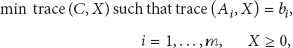$x(x-\mathrm{1})=\mathrm{0}$ . SDP has been shown to better approximate this constraint than LP relaxation (see [38] and references within). SDP is a convex optimization such that it optimizes a linear objective function over the intersection of the cone of positive semidefinite matrices with an affine space called a spectrahedron. The primal problem of the SDP problem is defined as follows: let ${𝒮}_q$ be the space of $q\times q$ real symmetric matrices, and we have

$$\begin{array}{l}\min \hspace{0.17em}\text{trace}\left(C,X\right)\text{such}\hspace{0.17em}\text{that}\hspace{0.17em}\text{trace}\left(A_i,X\right)=b_i,\\ \hspace{1em}\hspace{0.17em}\hspace{0.17em}\hspace{1em}\hspace{1em}\hspace{1em}\hspace{1em}\hspace{1em}i=\mathrm{1},\dots ,m,\hspace{1em}\mathrm{\hspace{0.17em}\hspace{0.17em}}X\ge \mathrm{0},\end{array}$$

(25)

where $C,A_i$ , $X\in {𝒮}_q$ for $i=\mathrm{1},\dots ,m$ , and $X>\mathrm{0}$ means X is inside of the cone of positive semidefinite matrices.

In this paper, we adopt the “Lift and Project” method proposed by Lovász and Schrijver [35] in solving the SDP formulation of the camera placement problem. We first generalize MIN and FIX into the following standard form:

$$\begin{array}{l}\text{Minimize}\mathrm{\hspace{0.17em}\hspace{0.17em}}-{\mathbf{c}}^T\mathbf{x}\\ \text{given}\mathrm{\hspace{0.17em}\hspace{0.17em}}\mathrm{\hspace{0.17em}\hspace{0.17em}}A\mathbf{x}\le \mathbf{b},\hspace{1em}{x}_i(x_i-\mathrm{1})=\mathrm{0},\end{array}$$

(26)

where x, b, c are column vectors and A is a matrix. The inequality constraint in (26) applies to each dimension. The “Lift and Project” process works as follows.

• (1)

  Define a variable matrix $Y=\{y_{i,j}\mid i,j=\mathrm{0,1},\mathrm{2},\dots ,n\}$ , where n is the length of vector x.

• (2)

  Replace each constraint $A_i\mathbf{x}\le b_i$ with a set of constraints $A_j\mathbf{x}·x_j\le b·x_j$ and $A_j\mathbf{x}·(\mathrm{1}-x_j)\le b·(\mathrm{1}-x_j)$ , $j=\mathrm{1,2},\dots n$ .

• (3)

  Replace each instance of x variable with y such that $x_i{x}_j=y_{i,j}$ , ${\hspace{0.17em}\hspace{0.17em}x}_i{x}_i=x_i=y_{i,i}=y_{\mathrm{0},i}$ for all $i,j$ .

• (4)

  Replace binary constraints $x_i(x_i-\mathrm{1})=\mathrm{1}$ with a constraint forcing Y to be positive semidefinite or $Y\succ \mathrm{0}$ .

• (5)

  Solve the SDP problem of Y and recover 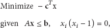$x_i=y_{\mathrm{0},i}$ .

It is shown in Section 5 that the “Lift and Project” process provides a much tighter bound than LP relaxation. In fact, we can get an even tighter relaxation by continuing to raise the dimension of variables. In [38], Laurent analyzed and compared three different hierarchical methods to obtain a series SDP relaxations of the 0-1 problem. However, in practical camera placement problems, the number of variables becomes large. Conducting more than one round of SDP relaxation will inevitably run into memory issues.

5. Experimental Results

In our previous paper [5], simulation using a walking humanoid and real-life experiments using a camera network with 7 cameras over a surveillance area of 7.6 m × 3.7 m were conducted to validate the model. We reused this model in this paper so that we could focus on how to solve the model efficiently. We propose three sets of simulation experiments to illustrate the strength and weakness of each proposed method. Firstly, we compare various fast and simple algorithms on a problem with a simple topology. Then, we compare them with more sophisticated algorithms on complex environments. Last but not least, we apply the LP and SDP relaxations on a small example to see how the SDP relaxation dramatically reduces the integrality gap.

For comparison, we only use the constraints in (10) and (18) with $k=\mathrm{2}$ . All experiments were conducted on a Duo core 2.8 GHz CPU with 3.2 GB RAM, with most code written in C linked to Matlab. The IP solver we used was in [39], and SDP solver we used was SDPA [40].

5.1. Environment with Simple Topology

In this section, we test our algorithms on a simple 2D square environment as in Figure 1(a). The blue hollow circles are discretized camera grid positions, and yellow solid stars are target grid positions. The blue arrows are the placed cameras. Here we have $\mathrm{28}$ camera positions and 49 tag positions. Each position is further divided into 8 grid points to represent different orientations. The total numbers of variables are $N_c=\mathrm{192}$ for cameras and $N_p=\mathrm{392}$ for targets.

Figure 1

Performance comparison of four approximation algorithms.

We first compare the running time for different algorithms and different sample sizes in Figure 1(b). In Figures 1(c)–1(f), we compare the results for different algorithms when the number of cameras varies. From those comparisons, we can make the following observations: (1) when the number of cameras is sufficiently large, the greedy algorithm has good approximation of IP solution with a fraction of the running time. However, when the number of cameras is small, the greedy algorithm provides much worse results due to its complete overlook of the combinatorial characteristics of the problem; (2) the sampling techniques can trade off performance with computational time; (3) using elements sampled from densities derived from the objective function significantly outperforms those from uniform random sampling; (4) the greedy heuristics generally outperforms other approximation methods. However, it can still be trapped in a local optimum regardless of the sample size. We will see that this disadvantage will incur big penalty when the environment becomes more complex.

5.2. Metropolis Sampling and Simulated Annealing on Complex Problems

As we can see above, for small and simple problems we can choose from the greedy algorithm (Algorithm 1), greedy heuristics (Algorithm 2), or sampling based on marginal distribution (Algorithm 3). Furthermore, these problems can also be solved by a standard IP solver in a reasonable running time. Now, we begin to look at much more complex environments.

In Figure 2, we show two complex environments generated by our camera placement GUI. We present the performances of IP solver, the greedy algorithm, Metropolis sampling, and simulated annealing (SA) approach in Table 2.

Table 2

Comparison of two Monte Carlo sampling methods with other algorithms.

	Environment 1		Environment 2
	Objective	Time (s)	Objective	Time (s)
IP	353	1552.4	2336	101320.6
Greedy	339	0.002014	2164	0.1362
Heuristic	344	0.0297	2029	0.440203
Metropolis	352	0.6784	2290	1.109044
Gibbs	344	17.14	2225	203.7
SA	350	1.957046	2336	7.739528

Figure 2

Two complex topologies. Black objects are obstacles and blue areas are secured areas with grid density 4 times higher than surroundings.

In order to demonstrate the merit of Simulated Annealing, Figure 3 shows three independent Markov chains using Metropolis sampling method with different single parameter T as a in (24). with higher temperature, we get more uniform samples which is useful for exploring the space. as temperature cool down we get less accepted samples but focus more on region with higher objective value.

Figure 3

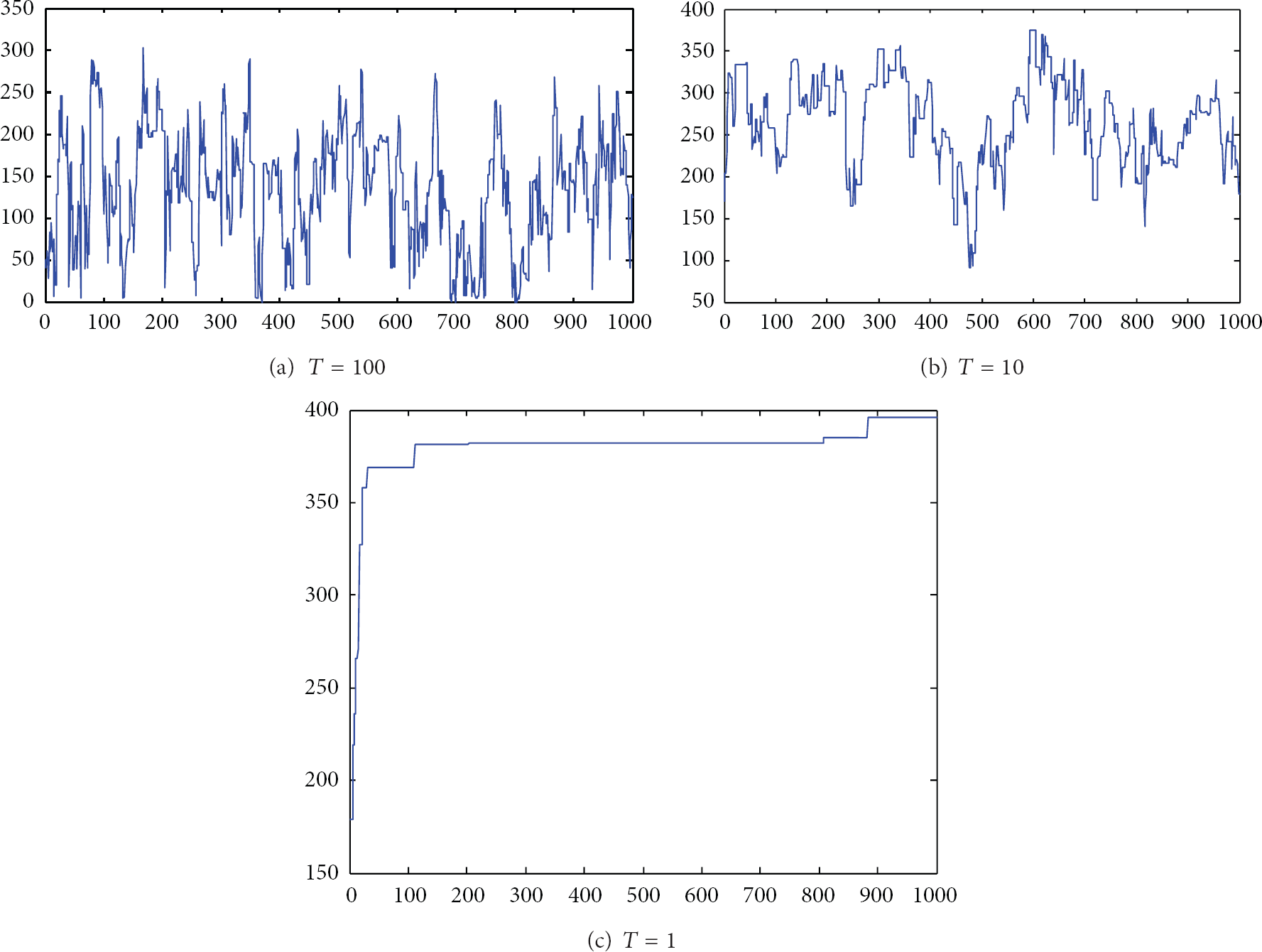
Three separate Metropolis Markov chain with different temperature.

We can conclude that both sampling algorithms are highly efficient when compared with the IP solver. We can further see the change of temperatures plays an important role in escaping the local optimums and exploring the entire search spaces.

5.3. LP Relaxation and SDP Relaxation

At last, we show the effectiveness of using SDP on relaxation on a simple and a moderate complex environment. The results are shown in Table 3. We can see that the SDP relaxation always gives a tighter bound comparing with LP relaxation. We visualize the camera grid variables for the simple topology in Figures 4(a) and 4(b), with the variable indexes in the x-axis and values in the y-axis. We can see that the SDP relaxation gives results closer to the binary with smaller objective value. In fact, in this particular example, the SDP relaxation solution coincides with the IP solution.

Table 3

Comparison of the objective values of SDP and LP relaxation.

	$\mathrm{56}$ grids, 2 cameras	$\mathrm{268}$ grids, $\mathrm{8}$ cameras
LP	11.5	32.25
SDP	11	31.34
Optimal	11	31

Figure 4

Comparison of IP and SDP relaxation.

6. Discussion

In this paper, we have presented and compared strengths and weaknesses of various well-known optimization frameworks to solve the generic camera placement problem including a greedy approach, MCMC methods, and LP and SDP relaxations.

In addition to our simulation study presented in this paper, it might be interesting to study how those algorithms can be combined together for solving the generic camera placement problem even more effectively. For example, the output of a greedy approach can be used as an initialization for the sampling methods. While SDP relaxations outperform the LP relaxation in terms of getting tighter bounds, it suffers from the dimension increase due to the “Lift and Project” process. Some dimension reduction approaches may be useful to reduce the problem size and apply more layers of SDP relaxations.

Additionally, it might be interesting to use other emerging optimization tools on our formulation. One example is least absolute shrinkage and selection operator (LASSO), which approximates the sparse approximation problem by a convex problem. For example, recall our MIN problem as follows:

$$\begin{array}{cc}& \min {\displaystyle \sum }_{i=\mathrm{1}}^{N_c}‍x_i\mathrm{\hspace{0.17em}\hspace{0.17em}}\mathrm{\hspace{0.17em}\hspace{0.17em}}\mathrm{\hspace{0.17em}\hspace{0.17em}}\text{such that}\hspace{0.17em}\hspace{0.17em}\mathbf{A}\mathbf{x}\le \mathbf{b}\mathbf{,}\mathrm{\hspace{0.17em}\hspace{0.17em}}{x}_i\hspace{0.17em}\hspace{0.17em}\text{is}\mathrm{\hspace{0.17em}\hspace{0.17em}}\text{binary}.\end{array}$$

(27)

One can formulate MIN problem in terms of the LASSO problem as follows:

$$\begin{array}{l}\text{min\hspace{0.17em}}{\parallel \mathbf{A}\mathbf{x}=\mathbf{b}\parallel }_{\mathrm{2}}+{\displaystyle \sum }_{i=\mathrm{1}}^{N_c}‍\left(x_i^{\mathrm{2}}-x_i\right)\\ \text{subject to\hspace{0.17em}}{\parallel \mathbf{x}\parallel }_1\le \lambda .\end{array}$$

(28)

This is a convex optimization problem and we might be able to solve the problem, by a convex optimization solver such as cvx [41].