Sage Journals: Discover world-class research

Abstract

The necessity to calibrate hot-wire probes against a known velocity causes problems at low velocities, due to the inherent inaccuracy of pressure transducers at low differential pressures. The vortex shedding calibration method is in this respect a recommended technique to obtain calibration data at low velocities, due to its simplicity and accuracy. However, it has mainly been applied in a low and narrow Reynolds number range known as the laminar vortex shedding regime. Here, on the other hand, we propose to utilize the irregular vortex shedding regime and show where the probe needs to be placed with respect to the cylinder in order to obtain unambiguous calibration data.

1. Introduction

The experimental investigation of turbulent flows has been performed in the last century to a large extent by means of hot-wire anemometry (HWA) which is an unrivalled technique compared to others, particularly due to its high frequency response and temporal resolution. Therefore, it is expected to continue to be used for the coming decades for the study of fluid dynamics as well as constitute a reference to other experimental methods.

Nevertheless, the technique has itself several limitations, in particular in wall-bounded turbulent flows or complex flow, such as wall interference and heat conduction to the wall [1], determination of the wire position relative to the wall [2] and also the effects of spatial resolution of the hot wire probe [3, 4]. Since hot wires are indirect methods, they need to be calibrated against a known velocity, which then can be related to the voltage reading from a HWA system. It is a common practice to calibrate hot wires against a pressure difference reading either from a pitot-static (so-called Prandtl) tube or across a calibration nozzle. In such case, another problem arises, namely, that of the low velocity calibration for velocities below say 1–3 m/s (see, e.g., [5, chapter 8.18], [6, chapter 4.7]), which is mainly caused by the inherent inaccuracy of pressure transducers at such small differential pressures [7].

For the calibration of hot wires at low velocities, several calibration techniques have been developed, such as modified calibration jets [8], the laminar pipe-flow method [9], the rotating disk method [10], methods exploring wall proximity effects [11, 12], and a variety of methods utilizing a moving [13 –15] or swinging probe in still air [16, 17], as well as the vortex shedding method [12, 18 –21]. In the present paper, we will focus on the vortex shedding calibration method, which has also been suggested in classical hot-wire literature, as, for example, in Perry [5] or Bruun [6]. The reason for preferring the vortex shedding method is its inexpensive and simple setup and especially its possibility to reach velocities that cannot easily be reached accurately with conventional pressure transducers.

2. Background

Since the discovery by Strouhal [22] that the frequency of the sound emitted by a wire exposed to a wind is linearly proportional to the wind speed itself and the proposal by Roshko [23] to expose this feature to measure the flow velocity, it is nowadays widely exploited in vortex flowmeters [24] as well as for the aforementioned calibration of hot wires at low velocities. Following the classical hot-wire literature [5, 6], it is suggested to employ a circular cylinder and the following relation between the Strouhal number, St = fD/U, and the cylinder Reynolds number, Re = UD/ν, proposed by Roshko [23]:

St = 0.212 (1 - \frac{21.2}{Re}), 50 < Re < 150,

(1)

St = 0.212 (1 - \frac{12.7}{Re}), 300 < Re < 2000,

(2)

where f is the fundamental vortex shedding frequency, D the cylinder diameter, U the flow velocity, and ν the kinematic viscosity. Since the velocity, which is aimed at being determined, appears in both the Strouhal and Reynolds numbers, it has been proposed to employ the so-called Roshko number defined as Ro = St Re = fD²/ν [23]. The obtained Ro-Re—relation is usually favored over the St-Re—relation given in (1) and (2), due to its linear and explicit nature [6]. When it comes to the exploitation of the vortex shedding phenomenon behind a circular cylinder, it has been a common practice to restrict the method to the laminar periodic vortex shedding region or the so-called stable range [12, 18 –20], that is, 30 to 48 < Re < 180 to 200 [25] described through (1). Since this regime is susceptible to oblique shedding which can alter the St-Re—relation [19, 26], special attention needs to be drawn to the end conditions of the cylinder as well as the interpretation of the measured frequency spectra [27].

While for flowmeter applications the Reynolds number range is commonly within the fully turbulent regime or the so called irregular range (although with quite noncircular shedder geometries that exhibit a much less Reynolds number-dependent range), only very few have employed the region beyond the transitional range inheriting the discontinuities in the St-Re—relation [25, 28], which occur between the two Reynolds number regions defined through (1) and (2). While there were practical reasons to favor the stable range for calibration purposes in the past, for example, due to the employment of zero-crossing counters [18, 29] or signal generators and oscilloscopes to determine the vortex shedding frequency by means of the so-called Lissajous figure [5, 30], the shedding frequency can nowadays simply be determined by fast Fourier transform (FFT) algorithms. Also, the utilization of the irregular regime would avoid the aforementioned difficulties related to the appearance of oblique vortex shedding.

In the present paper the vortex shedding calibration method for hot-wires is employed in the irregular region and it is shown to be a robust and reliable technique.

3. Experimental Setup and Measurement Technique

The experimental data was obtained in the Minimum Turbulence Level (MTL) wind tunnel located at the Royal Institute of Technology (KTH) in Stockholm. The test section is 7 m long with a cross-sectional area of 0.8 × 1.2 m² (height × width). The maximum speed with an empty test section is 70 m/s, and the streamwise velocity disturbance level is less than 0.025% of the free stream velocity. The air temperature can be regulated within ± 0.05°C by means of a heat exchanger. For further information regarding the flow quality in the MTL wind tunnel, the reader is referred to Lindgren and Johansson [31]. Two circular cylinders with a nominal diameter, D, of 8 and 12 mm (giving a length-to-diameter ratio of 150 and 100, resp.) were spanned at the middle of the wind tunnel in terms of height and length. Throughout the remainder of the paper, the streamwise, vertical, and spanwise (i.e., along the cylinder) directions are denoted by x, y, and z, with the origin set at the centre of the cylinder as depicted in Figure 1.

Figure 1:

Schematic of the coordinate system centered around the cylinder of diameter D. The streamwise, vertical, and spanwise directions are denoted by x, y, and z, respectively. Hot-wire measurements at constant free stream velocities were performed at the intersection points of the red x-y grid. Positions indicated through blue crosses or crossed-circles and denoted by roman numerals will be referred to and described throughout the paper.

The hot-wire probe used for the present measurements is a standard straight hot wire with a platinum wire of nominal diameter of 5 microns and a length of 1 mm. The hot-wire was calibrated in situ in the free stream against a Prandtl tube, which was connected to a micromanometer of type FC0510 (Furness Control Limited), from which also the ambient temperature and pressure were obtained. Calibration curves were taken at the beginning and end of each set of measurements and fitted to a calibration relation proposed by Johansson and Alfredsson [32]

U = k_{1} {(E^{2} - E_{0}^{2})}^{1 / n} + k_{2} {(E - E_{0})}^{1 / 2},

(3)

where E and E₀ are the anemometer output voltages at velocities U and zero, respectively, and k₁, k₂, and n are calibration constants. While the first term of (3) is related to the classical King's law [33], the second term takes account on the effect of natural convection, which becomes important at low velocities.

The hot-wire anemometer system used is a DANTEC StreamLine 90N10 frame in conjunction with a 90C10 constant temperature anemometer module. An offset and gain was applied to the top of the bridge voltage in order to match the voltage range of the 16 bit A/D converter used.

4. Vortex Shedding Calibration Method

4.1. Placement of the Hot-Wire Probe

When it comes to the application of the vortex shedding phenomenon for calibration purposes of hot-wires, there are barely any guidelines in terms of where the probe should be placed both in order to measure the hot-wire voltage related to the free stream velocity, E, as well as the vortex shedding frequency, f. The reason for this is probably due to the fact that “most research in the past has been focused on circular cylinders” [25] when it comes to bluff body wakes, and in turn, there is a large body of literature regarding the near-field spreading rates of cylinder wakes, which can be consulted to find a suitable location for various Reynolds number ranges. Furthermore, due to the presence of an absolute instability in the Kármán vortex sheet, the shedding frequency can be “felt” wherever the probe is placed. Nevertheless, it was decided to map the wake region for both utilized cylinders at a free stream velocity range around 1 and 4 m/s.

In the following results from the cylinder with a nominal diameter of 12 mm are shown to demonstrate the method, whereas results for the cylinder with the diameter of 8 mm are also provided later. Figure 2 shows the premultiplied power spectral density map for the hot-wire voltage signal at 1.5D downstream of the cylinder across the y-direction for U_∞ = 4.2 m/s, where P_ee is the power spectral density function of the measured signal and f is the frequency domain. The frequency domain in the horizontal axis is normalized with the fundamental frequency f_p regarding the applied free stream velocity. The fundamental frequency f_p is hereby determined by finding the maximum of the premultiplied spectra, that is, fP_ee, without any ambiguity across the wake in the y-direction, except along the centerline of the wake, where the picked up frequency is an integer multitude (harmonic) of the fundamental frequency, f_p.

Figure 2:

Premultiplied power spectral density map for the voltage signal from the hot-wire at x/D = 1.5 across the y-plane, indicated through I in Figure 1, for U_∞ = 4.2 m/s. The premultiplied spectral amplitudes have been scaled with the variance of the voltage signal in order to make the spectral peaks also outside the wake region. Note that the spectral plot along the visible centerline of the wake (i.e., y/D = 0; red line) displays a higher amplitude than the fundamental frequency. The robustness of the determined fundamental frequency is also emphasized through the red line parallel to the y-axis.

In order to ensure that the measured behavior is not only a local observation at one downstream location, measurements in the x-y-plane have been performed at all intersection points of the depicted measurement grid in Figure 1. The result is depicted in Figure 3 where the white area is illustrating the region in which the fundamental shedding frequency is captured. As apparent from this figure, the fundamental shedding frequency, f_p, can unambiguously be determined across the entire wake in the range 1 < x/D < 6, except along the centerline, where the amplitude of the harmonic dominates the fundamental frequency. Although the fundamental frequency is present for the region $| y / D | > 5.5$ , it can not unambiguously be determined, since its amplitude is comparable to that of the background level. A quite similar result can also be obtained by directly taking the maximum of P_ee; however, favoring the premultiplied form helped to suppress low-frequency modulations as well as enhance the fundamental peak and thereby yield maps free of wrinkles.

Figure 3:

Downstream evolution (i.e., x/D) of the determined frequencies for the same experimental conditions as in Figure 2 through measurements at all intersection points shown in Figure 1. The fundamental frequency, f_p, was captured in the white area, whereas its harmonic was in the red area. No dominant frequency was captured in the blue area. Vertical dashed line corresponds to the downstream location that will be employed later on for calibration purposes.

While the positioning of the hot wire for the determination of the fundamental frequency has been clarified, the position for the measurement of the mean voltage of the hot-wire that is related to the free stream velocity, that is, E, needs to be checked. The surface plot of the mean streamwise velocity depicted in Figure 4 clearly shows that irrespective of the downstream location, $| y / D | > 5.5$ appears to be suitable to obtain the free stream velocity. Note also that the turbulence intensity reaches the free stream level much quicker (not shown here) and therefore will not bias the obtained mean voltage corresponding to the free stream conditions. A less stringent lower threshold can also be used for further downstream positions. This rule of thumb is also valid when taking the results from the lower velocity as well as the smaller diameter into account. Hence, taking all results with some tolerances into account, it is recommendable to determine the fundamental shedding frequency for 1 < x/D < 6 within $1 < | y / D | < 4$ , while the hot-wire voltage related to U_∞ should be acquired at $| y / D | > 5.5$ . These recommendations are also close to those given by Ardekani [21], who gave $2.2 < | y / D | < 2.9$ for 3 < x/D < 6, for the regime bridging, the stable and irregular regimes, namely, 100 < Re < 430, in order to determine both E and f simultaneously. Nevertheless, it seems more appropriate to comply to the limits given here, due to the extended Re—range employed, in order to obtain an unbiased hot-wire voltage which is related to the voltage in the free stream.

Figure 4:

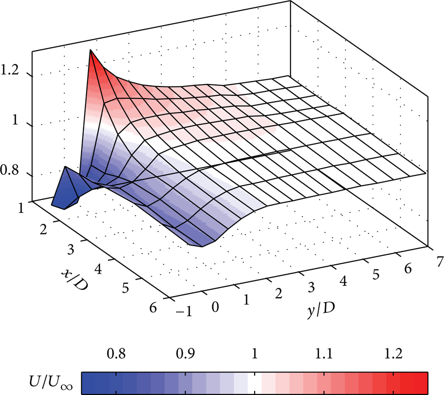
Surface plot of the evolution of the mean streamwise velocity scaled by the free stream velocity in the x-y plane. White shaded areas denote U within ±1% of U_∞.

Having established the two regions in which (1) the fundamental frequency of the vortex shedding can be obtained from the voltage signal of the hot-wire and (2) the region where the hot-wire is exposed to the mean voltage of the hot-wire that is related to the free stream velocity, it becomes obvious that a single hot-wire problem can be utilized for both purposes. Traditionally, one hot-wire is used to detect the shedding frequency, while a second—the one that is calibrated—is measuring the voltage related to the free stream velocity. For smaller wind tunnels, where blockage might influence the quantitative results presented here, maps as shown in Figures 3 and 4 can easily be obtained and used for future calibrations.

4.2. Application of Vortex Shedding Calibration Method

Having established where to place the hot-wire probe in order to pick up the fundamental frequency, f_p, as well as an unbiased mean voltage from the hot wire, E, hot-wire calibrations with both the 8 and 12 mm cylinders covering a velocity range from as low as 0.15 m/s up to 10 m/s were performed. While the low velocity end was restricted due to the stability of the MTL wind tunnel, the higher end was mainly used to have a sufficient overlapping region with the conventional hot-wire calibration against a Prandtl tube. For the performed calibrations, the hot-wire was placed 3D downstream the cylinder, and measurements were taken at y/D = 2.5 and 6 (indicated withII andIII in Figure 1) for f_p and E, respectively, for each tunnel speed.

The result of such a calibration is depicted in Figure 5, where the premultiplied spectra are mapped for different tunnel speeds and hence different E. Utilization of (1) and (2) yields the free stream velocity, which coupled with the measured voltage E provides the data set for the calibration. Results from both cylinders have been depicted together with a conventional calibration by means of a Prandtl tube in Figure 6. Note that for velocities beyond approximately 2.5 and 4 m/s for the 12 and 8 mm cylinders, respectively, the relation given in (2) tends to underestimate the determined velocity, since the St-Re—relation reaches a maximum and starts to decay from Re ≈ 2000 on. In order to utilize the calibration points beyond this Re, the St-Re—relation for Re > 2000 was taken from well-established empirical data [25, 34, 35]. Although, “in practice, (2) is often also applied for higher Reynolds numbers, [·], it should not be used for Re > 5000”[35]. Nevertheless, it should be noted that for velocities above 2 m/s, the conventional calibration by means of a Prandtl tube is favored compared to any other method, and therefore, the explained extension of the vortex shedding method for higher velocities is barely an esthetic operation. The Reynolds number range utilized for the vortex shedding calibration method in the data illustrated in Figure 6 is presented in Table 1 for both cylinder diameters. The calibration constants,n, k₁, and k₂, for the fitted calibration data to the modified King's law relation, that is, (3), are also provided in the table for better comparison between different calibration curves.

Table 1:

Calibration cases depicted in Figure 6 with the utilized Reynolds number range and the coefficients for the best fit to the modified King's law, that is, (3). C₃ corresponds to the conventional calibration method.

Case	Cylinder dia. (mm)	Re	Fitting coefficients
Case	Cylinder dia. (mm)	Re	n	k ₁	k ₂

C₁	8	280–5500	0.4797	2.671	1.884
C₂	12	140–8200	0.4896	2.723	1.775
C₃	—	—	0.4874	2.743	1.828

Figure 5:

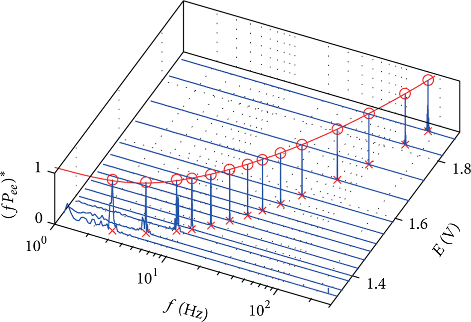
Premultiplied power spectral density map for the voltage signal from a hot-wire located 3D downstream of the cylinder for different U_∞. The power spectral density is computed from measurements within the wake (i.e.,y/D = 2.5), while the mean voltage from the hot wire is obtained outside the wake region (i.e., y/D = 6). The asterisk denotes normalization of the premultiplied spectral amplitudes to unity in order to visualize the fundamental peaks as well as to ease visualization of the hot-wire calibration relation. Note that the frequency axis is plotted in logarithmic scale in order to emphasize the low velocity (i.e., frequency) region. Obtained calibration points for E versus f_p are highlighted by red circles, and the red solid line is (3) fitted to the data pairs.

Figure 6:

Conventional hot-wire calibration plot and magnified view on the low velocity region (insert). Blue stars and dashed line are from a conventional calibration against a Prandtl tube, and red circles and solid line are from the vortex shedding method (same data as depicted in Figure 5), while the black squares are obtained similarly but with a cylinder diameter of 8 mm, instead of 12 mm. The lines are obtained from (3) (which inherently enforces that the curve goes through E₀, denoted by +) fitted to the corresponding data.

Coming back to Figure 6, the general agreement between the conventional Prandtl tube calibration and the results from the vortex shedding calibration obtained with two different cylinder diameters over more than an order of magnitude in velocity can be appreciated. Hence, the utilization of the irregular vortex shedding regime is justified. Although the first and first two calibration points from the 8 and 12 mm cylinders, respectively, are within the transitional regime, there appears to be no marginal difference in U when taking various St-Re—relations for the transitional regime, when displayed in such a plot. Nonetheless, the obtained velocities could differ up to ±3% in this narrow Re—range, but such a deviation can still be considered fairly accurate when compared to readings from pressure transducers at differential pressures around or even below 1 Pa.

5. Summary and Conclusions

Hot-wire anemometry is since a long time the standard measurement technique in turbulent air flows. Its indirect working principal, however, calls for calibration against a known velocity to which the voltage from the hot-wire anemometer can be related. Commonly, the hot wire is calibrated against the pressure difference reading from a Prandtl tube; however, at low velocities, this becomes problematic, due to the inherent inaccuracy of pressure transducers at low differential pressures.

In the present work we have demonstrated the so-called vortex shedding calibration method which has been known in the past as the simplest and most accurate method to calibrate hot wires at very low velocities but has only been utilized to a very narrow Reynolds number regime. Here, we propose to utilize also the irregular vortex shedding regime and thereby extend the Reynolds number range.

The flow field behind a circular cylinder has been mapped by means of hot-wire anemometry down to 6D. From these measurements, it could be inferred that both the fundamental vortex shedding frequency as well as the hot-wire voltage related to the free stream velocity can unambiguously be determined irrespective of downstream position for 1 < y/D < 4 and $| y / D | > 5.5$ , respectively. The proposed extension of the well-established vortex shedding calibration method has been demonstrated to yield accurate calibration data for hot-wires over more than a decade in velocity for a selected cylinder diameter down to 0.15 m/s (restricted due to the employed wind tunnel and not the method itself).

Footnotes

Acknowledgments

This research was done within KTH CCGEx, a centre supported by the Swedish Energy Agency (STEM), Swedish Vehicle Industry, and KTH. Professor P. Henrik Alfredsson is acknowledged for stimulating discussions.

References

Durst

and Zanoun

, “Experimental investigation of near wall effects on hot-wire measurements,” Experiments in Fluids, vol. 33, no. 1, pp. 210–218, 2002.

Fransson

J. H. M.

, and Henrik Alfredsson

, “On near wall measurements of wall bounded flows—the necessity of an accurate determination of the wall position,” Progress in Aerospace Sciences, vol. 46, no. 8, pp. 353–387, 2010.

Hutchins

Nickels

T. B.

Marusic

, and Chong

M. S.

, “Hotwire spatial resolution issues in wall-bounded turbulence,” Journal of Fluid Mechanics, vol. 635, pp. 103–136, 2009.

Örlü

and Alfredsson

P. H.

, “On spatial resolution issues related to time-averaged quantities using hot-wire anemometry,” Experiments in Fluids, vol. 49, no. 1, pp. 101–110, 2010.

Perry

A. E.

, Hot-Wire Anemometry, Clarendon Press, 1982.

Bruun

H. H.

, Hot-Wire Anemometry: Principles and Signal Analysis, Oxford University Press, New York, NY, USA, 1995.

Lekakis

, “Calibration and signal interpretation for single and multiple hot-wire/hot-film probes,” Measurement Science and Technology, vol. 7, no. 10, pp. 1313–1333, 1996.

Grandchamp

Van Hirtum

, and Pelorson

, “Hot film/wire calibration for low to moderate flow velocities,” Measurement Science and Technology, vol. 21, Article ID 115402, 2010.

Yue

and Malmström

, “A simple method for low-speed hot-wire anemometer calibration,” Measurement Science and Technology, vol. 9, no. 9, pp. 1506–1510, 1998.

10.

Özahi

Özdinç Çarpinlioğlu

, and Yaşar Gündoğdu

, “Simple methods for low speed calibration of hot-wire anemometers,” Flow Measurement and Instrumentation, vol. 21, pp. 166–170, 2010.

11.

Janke

, Hot Wire in Wall Proximity. Advances in Turbulence, vol. 1, Springer, 1987.

12.

Lanspeary

, Establishing very low speed, disturbance-free flow for anemometry in turbulent boundary layers [Ph.D. thesis], University of Adelaide, Adelaide, Australia, 1998.

13.

Heikal

Antoniou

, and Cowell

T. A.

, “A rig for the static calibration of constant-temperature hot wires at very low velocities,” Experimental Thermal and Fluid Science, vol. 1, no. 2, pp. 221–223, 1988.

14.

Chua

L. P.

H.-S.

, and Zhang

, “Calibration of hot wire for low speed measurements,” International Communications in Heat and Mass Transfer, vol. 27, no. 4, pp. 507–516, 2000.

15.

Al-Garni

A. M.

, “Low speed calibration of hot-wire anemometers,” Flow Measurement and Instrumentation, vol. 18, no. 2, pp. 95–98, 2007.

16.

Zabat

Browand

F. K.

, and Plocher

, “In-situ swinging arm calibration for hot-film anemometers,” Experiments in Fluids, vol. 12, no. 4–5, pp. 223–228, 1992.

17.

Guellouz

M. S.

and Tavoularis

, “A simple pendulum technique for the calibration of hot-wire anemometers over low-velocity ranges,” Experiments in Fluids, vol. 18, no. 3, pp. 199–203, 1995.

18.

Kohan

and Schwarz

W. H.

, “Low speed calibration formula for vortex shedding from cylinders,” Physics of Fluids, vol. 16, no. 9, pp. 1528–1529, 1973.

19.

Lee

and Budwig

, “Two improved methods for low-speed hot-wire calibration,” Measurement Science and Technology, vol. 2, no. 7, pp. 643–646, 1991.

20.

Papangelou

, “A “robust” vortex-shedding anemometer,” Experiments in Fluids, vol. 14, no. 3, pp. 208–210, 1993.

21.

Ardekani

M. A.

, “Hot-wire calibration using vortex shedding,” Measurement, vol. 42, no. 5, pp. 722–729, 2009.

22.

Strouhal

, “Ueber eine besondere Art der Tonerregung,” Annalen der Physik und Chemie, vol. 241, pp. 216–251, 1878.

23.

Roshko

, “On the development of turbulent wakes from vortex streets,” NACA Tech Note 2913, 1953.

24.

Laurantzon

Örlü

Segalini

, and Alfredsson

P. H.

, “Time-resolved measurements with a vortex flowmeter in a pulsating turbulent flow using wavelet analysis,” Measurement Science and Technology, vol. 21, Article ID 123001, 2010.

25.

Zdravkovich

, Flow Around Circular Cylinders: Fundamentals, Oxford University Press, New York, NY, USA, 2003.

26.

Lee

and Budwig

, “A study of the effect of aspect ratio on vortex shedding behind circular cylinders,” Physics of Fluids A, vol. 3, no. 2, pp. 309–315, 1991.

27.

Gerich

and Eckelmann

, “Influence of end plates and free ends on the shedding frequency of circular cylinders,” Journal of Fluid Mechanics, vol. 122, pp. 109–121, 1982.

28.

Williamson

C. H. K.

, “Vortex dynamics in the cylinder wake,” Annual Review of Fluid Mechanics, vol. 28, pp. 477–539, 1996.

29.

Gaster

, “Vortex shedding from circular cylinders at low Reynolds numbers,” Journal of Fluid Mechanics, vol. 46, pp. 749–756, 1971.

30.

Kovasznay

L. S. G.

, “Hot-wire investigation of the wake behind cylinders at low Reynolds numbers,” Proceedings of the Royal Society A, vol. 198, pp. 174–190, 1949.

31.

Lindgren

and Johansson

A. V.

, “Evaluation of the flow quality in the MTL wind-tunnel,” Tech. Rep. TRITA-MEK, 2002:13, Royal Institute of Technology, Stockholm, Sweden.

32.

Johansson

A. V.

and Alfredsson

P. H.

, “On the structure of turbulent channel flow,” Journal of Fluid Mechanics, vol. 122, pp. 295–314, 1982.

33.

King

, “On the convection of heat from small cylinders in a stream of fluid: determination of the convection constants of small platinum wires with applications to hot-wire anemometry,” Philosophical Transactions of the Royal Society A, vol. 214, pp. 373–432, 1914.

34.

Norberg

, “Experimental investigation of the flow around a circular cylinder: influence of aspect ratio,” Journal of Fluid Mechanics, vol. 258, pp. 287–316, 1994.

35.

Fey

König

, and Eckelmann

, “A new Strouhal-Reynolds-number relationship for the circular cylinder in the range 47 < Re < 2 × 10 ₅,” Physics of Fluids, vol. 10, no. 7, pp. 1547–1549, 1998.

Hot-Wire Calibration at Low Velocities: Revisiting the Vortex Shedding Method

Abstract

1. Introduction

2. Background

3. Experimental Setup and Measurement Technique

4. Vortex Shedding Calibration Method

4.1. Placement of the Hot-Wire Probe

4.2. Application of Vortex Shedding Calibration Method

5. Summary and Conclusions

Footnotes

Acknowledgments

References