Sage Journals: Discover world-class research

Abstract

Thermal load is an important factor that must be taken into account during the procedure of bridge design and structural condition evaluation especially for those statically indeterminate bridges and cable-supported bridges. This paper presents an overview of current research and development activities in the field of thermal load in bridge, in which emphasis is placed on the thermal load models established by numerical analysis and field measurement. The theoretical formulations and boundary conditions of heat transfer in bridge are firstly outlined. And then, the states of the art of numerical solutions for temperature distribution in bridge including finite difference method and finite element method are reviewed in detail. Following that, the progress on thermal load in three types of representative bridges that are concrete bridge, steel-concrete composite bridge, and steel bridge based on field measurement data is discussed extensively. Finally, some existing problems and promising research efforts about thermal load in bridge are remarked.

1. Introduction

Different forms of bridges, such as cable-supported bridge, arch bridge, multispan continuous bridge and simple supported bridge, which are key elements of the highway infrastructure, have been built throughout the world to fulfill the requirements of modern society for advanced transportation [1–4]. Recent advances of design methodologies and construction technologies have made it possible to construct bridges with great size. Up to now, the span of bridge exceeds 1900 m, and the depth and the width of the box girder are more than 13 m and 35 m, respectively [5–7]. It is well known that the service life of those bridges almost exceeds 50 years or even 100 years sometimes. During the lifetime, it is inevitable that bridges are subjected to daily, seasonal, and yearly repeated cycles of heating and cooling induced by solar radiation and surrounding air. The up and down temperatures in structural components may cause nonlinear thermal load that influences the performance of bridges significantly.

In practice, the variation of temperatures affects bridges in a complicated manner. From the point of view of global response, uniform temperature changes cause large overall expansion and contraction in bridge components. On one hand, the deformation induces the shift of structural dynamic characteristics, which has significant influence on the results of damage identification using vibration-based methods. Researchers from Los Alamos National Laboratory found that the first three natural frequencies of the Alamosa Canyon Bridge varied about 4.7%, 6.6%, and 5.0% during a 24 h period as the temperature of the bridge deck changed by approximately 22°C [8, 9]. Liu and DeWolf [10] reported that, during a 1-year measurement, the first three frequencies of a curved concrete box bridge decreased by 0.8, 0.7, and 0.3% as temperature increased by one degree Celsius. Xu and Wu [11] analyzed the effects of change in environmental temperature on the frequencies and mode shape curvatures of a cable-stayed bridge considering seasonal temperature difference and sunshine temperature difference by finite element method. The outcome of the study indicates that changes in dynamic characteristics of the bridge due to damage in girders or cables may be smaller than those due to variations in temperature. On the other hand, the continuous expansion and contraction may damage critical member of bridge, such as expansion joint, bearing, and anchor head. The service life and interval for replacement of expansion joints rely to a great extent on the cumulative displacements. Ni et al. [12] concluded that the movements of the expansion joints are highly correlated with the effective temperature based on the long-term monitoring data of expansion joint displacement and bridge temperature. Xu et al. [13] investigated the displacement responses of the Tsing Ma Bridge in Hong Kong from 1997 to 2005 using the measurement data recorded by structural health monitoring system. It was found that the longitudinal displacement responses of the bridge towers, deck sections, and cables show strong linear relationships with the effective deck temperature, and the vertical displacement of the deck sections and cables at the main span is also correlated with the effective deck temperature. And from the point of view of local response, temperature variations result in considerable thermal stresses if the thermal deformation of bridge components is restricted, which may be comparable to that induced by dead or live load. In concrete bridge, such stresses can initiate tensile failure for the low tensile strength of concrete. Those minute cracks due to tension may subsequently grow into large cracks that allow the reinforcing steel to be exposed to possible corrosion. The effect of corrosions of reinforced concrete on new and existing structures can be aggravated as a result of these thermal cracks in addition to the existing service load cracks [14]. In steel bridge, the fatigue performance of weld joints is degraded dramatically when those stresses superpose the welding residual stresses and the stresses induced by service load. Furthermore, the thermal stresses tend to change the stress distribution in steel and concrete of steel-concrete composite bridge and cause deterioration in material. Therefore, thermal load is an important factor that should be considered during the whole life of bridge. Failure to closely understand temperature effects may result in considerable damages in bridge and false alarms of structural deterioration [15, 16].

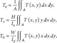
According to the different effects, the thermal load can be classified as effective temperature, vertical temperature difference (temperature gradient), and horizontal temperature difference. The effective temperature, which accounts for the expanding and contracting of bridge components in the longitudinal direction, is the weighted mean value of temperature distributed along the cross section. The vertical temperature difference, which results in supplementary internal axial forces and bending moments in vertical plane when the section ends are restrained, refers to the difference of temperatures between the top surface and other levels in the cross section [17]. The horizontal temperature difference, which induces secondary internal axial forces and bending moments in horizontal plane if the deformation is constrained, represents the difference of temperatures between two positions on the same level in the cross section. The effective temperature and vertical temperature difference are included in almost all bridge design specifications. According to the definition, the effective temperature $T_{e}$ , vertical temperature difference $T_{v}$ , and horizontal temperature difference $T_{h}$ can be expressed as

\begin{matrix} T_{e} = \frac{1}{A} \iint_{A} T (x, y) d x d y, \\ T_{v} = \frac{H}{I_{x}} \iint_{A} T (x, y) y d x d y, \\ T_{h} = \frac{W}{I_{y}} \iint_{A} T (x, y) x d x d y, \end{matrix}

(1)

where A represents the area of the cross section;

T (x, y)

represents the two-dimensional temperature over the cross section, and x and y represent the horizontal and vertical axis of the cross section, respectively;

I_{x}

and

I_{y}

represent the moments of inertia of the section about the x and y axes, respectively; and H and W represent the depth and width of the cross section, respectively.

Early in the 1960s, Zuk [18] started a study on the thermal behaviour of highway bridges. It was concluded that the thermal load is affected by air temperature, wind, humidity, intensity of solar radiation, and material type after investigation on several bridges. Subsequently, researchers and engineers were aware of the nonlinear temperature distribution developed within a bridge gradually. Study on thermal load in different bridges subjected to the change of environmental factors has been performed all over the world. Those researches can be roughly divided into three categories, which are theoretical method, numerical approach, and field measurement. The theoretical method is aimed to pursue the closed-form solutions of the heat transfer equation and reveal the temperature distribution in bridges, which must employ a series of assumptions. The numerical approach solves the hear transfer equation by finite element method or finite difference method, which can give acceptable results if the input parameters are adjusted properly. The field measurement obtains the temperature distribution by temperature sensors installed on full-scale bridges in real environment, which provides the most meaningful thermal load of bridges. Each one has its advantages and disadvantages. It is difficult to say that one method is better than others.

In this paper, the research progress of thermal load in bridge over the past several decades is reviewed in detail. A brief overview of the theoretical model of heat transfer in bridge is outlined in Section 2. And then, the numerical approach used to solve the theoretical model is provided in Section 3. After that, the field measurement results of concrete bridges, steel-concrete composite bridges, and steel bridges, in addition to temperature sensor and data processing methodology, are investigated in Section 4. Finally, the conclusions and recommendations are given in Section 5. This paper is not intended to list all literatures about thermal load in bridge but to exhibit some representative achievements. Through pertinent assessment, the problems and promising directions about the topic of thermal load in bridge are expected to be extracted for future research.

2. Theoretical Model

Temperature distribution within a bridge is governed by heat conduction inside its body and the convective and radiative heat exchange with the surrounding environment. The heat conduction can be modeled by applying the principle of the Fourier's law, and the heat exchange is formulated by boundary condition.

In 1822, Fourier stated that the rate of heat transfer is proportional to the temperature gradient in a solid and established the well-known Fourier partial differential equation, which is [14, 19, 20]

\begin{matrix} \frac{\partial}{\partial x} (k_{x} \frac{\partial T}{\partial x}) + \frac{\partial}{\partial y} (k_{y} \frac{\partial T}{\partial y}) + \frac{\partial}{\partial z} (k_{z} \frac{\partial T}{\partial z}) + Q = c ρ \frac{\partial T}{\partial t}, \end{matrix}

(2)

where

x, y

, and z represent Cartesian coordinates, which are the horizontal, vertical, and longitudinal axes of bridge, respectively;

k_{x}

k_{y}

, and

k_{z}

represent thermal conductivities corresponding to the

x, y

, and z Cartesian axes; t represents time; T represents temperature at position

(x, y, z)

at time t; Q represents the rate of heat generated per unit volume; c represents coefficient of specific heat of medium; and ρ represents density of medium.

For a bridge exposed to solar radiation, it can be assumed that the material is continuum, isotropic, and homogeneity. Based on the results investigated by McClure et al. from the field measured data obtained by thermocouples [21], the thermal flow along the direction of the longitudinal axis can be normally neglected. After the hydration of cement in concrete bridge and the action of welding in steel bridge, the rate of generating heat Q can be set to zero. Therefore, (2) can be simplified as a two-dimensional model as

\begin{matrix} k (\frac{\partial^{2} T}{\partial x^{2}} + \frac{\partial^{2} T}{\partial y^{2}}) = c ρ \frac{\partial T}{\partial t}, \end{matrix}

(3)

where k represents thermal conductivity.

If only the vertical temperature gradient is considered, the temperature differential in x direction can be ignored. Equation (3) can be further rewritten as

\begin{matrix} k \frac{\partial^{2} T}{\partial y^{2}} = c ρ \frac{\partial T}{\partial t} . \end{matrix}

(4)

Considering heat exchange, the boundary condition associated with (3) is expressed as follows [20]:

\begin{matrix} k (\frac{\partial T}{\partial x} n_{x} + \frac{\partial T}{\partial y} n_{y}) + q = 0, \end{matrix}

(5)

where

n_{x}

and

n_{y}

represent the direction cosines of the unit outward vector normal to the boundary surfaces, and q represents the rate of heat exchanged between the boundary and the environment per unit area.

The heat exchange between the boundary of bridge and the environment is very complex, as shown in Figure 1. It is composed of three principal mechanisms: solar radiation, convection, and thermal irradiation. And the solar radiation is generally considered to be the most important one among the three mechanisms. The rate of heat exchange q is the sum of the three actions,

\begin{matrix} q = q_{s} + q_{c} + q_{r}, \end{matrix}

(6)

where

q_{s}

represents the solar radiation;

q_{c}

represents the convection; and

q_{r}

represents the irradiation from the surface to the surrounding air. Each of these parameters varies with the positions considered and the time.

Figure 1

Heat exchange between the boundary and the environment.

The rate of heat due to solar radiation $q_{s}$ , that is, shortwave radiation, received by the bridge can be expressed as [22]

\begin{matrix} q_{s} = α I, \end{matrix}

(7)

where α represents the dimensionless absorptivity of the surface of the bridge; I represents the total solar radiation on a tilted surface, which depends upon the point considered and the incidence angle of sun rays. In shaded areas, I is equal to 0.

The total solar radiation on the inclined surface can be formulated as a function of variables related to the location and orientation of the bridge (latitude, altitude, solar declination, transmission factor, the bridge azimuth, etc.) [23]. Another way obtaining the value of this climatic parameter starts from the beam (direct) radiation, diffuse radiation, and ground-reflected radiation and using sinusoidal functions, which is in good agreement with experimental results [14]. In this way, the total solar radiation on the inclined surface is divided into three components: beam (direct) radiation, diffuse radiation, and ground-reflected radiation [20, 22, 24]. Beam radiation, the major component of solar radiation, is the solar radiation received from the sun not scattered by the atmosphere. It is often referred to as direct solar radiation. Diffuse radiation is the solar radiation received from the sun after its direction is changed by the atmosphere through a process of scattering. This makes things, even indoors, visible without direct sunlight. Ground-reflected radiation is radiation reflected from the ground cover and bodies of water on the surface of the earth. Although beam radiation is the major component causing nonuniform temperature distribution in the bridge, diffuse radiation and ground-reflected radiation are not negligible [25]. So the total solar radiation can be calculated by the equation presented by Duffie and Beckman [22] and Orgill and Hollands [24], which is

\begin{matrix} I = I_{b} \frac{\cos θ}{\cos θ_{z}} + I_{d} (\frac{1 + \cos β}{2}) + (I_{b} + I_{d}) η (\frac{1 - \cos β}{2}), \end{matrix}

(8)

where

I_{b}

and

I_{d}

represent the beam solar radiation and the diffuse radiation on a horizontal surface, respectively; θ represents the angle of incidence (the angle between the beam radiation on a surface and the normal to that surface);

θ_{z}

represents the zenith angle; β represents the slope, that is, the angle between the plane surface in question and the horizontal surface; η represents the diffuse ground reflection.

The heat lost to or gained from the surrounding air by convection as a result of temperature differences between the bridge surface and the air is given by Newton's law of cooling as [23]

\begin{matrix} q_{c} = h_{c} (T_{s} - T_{a}), \end{matrix}

(9)

where

h_{c}

represents the convection coefficient of heat transfer;

T_{s}

represents the temperature of the surface contact with the air; and

T_{a}

represents the air temperature. Because of the complexity of heat transfer by convection, the convection coefficient of heat transfer

h_{c}

is a function of many variables such as wind speed, surface roughness, and geometric configuration of the exposed structure. The accurate analytical expression that describes those factors is unavailable now.

The heat transfer between the bridge surface and the surrounding atmosphere due to thermal irradiation, that is, long wave radiation, produces a nonlinear boundary condition which can be modeled by Stefan-Boltzmann radiation law as [20, 23, 26]

\begin{matrix} q_{r} = C_{s} e [(T_{s} + T^{*}) - (T_{a} + T^{*})], \end{matrix}

(10)

where

C_{s}

represents the Stefan-Boltzmann constant; e represents the emissivity coefficient relating the radiation of the bridge surface to that of an ideal black body (

0 \leq e \leq 1

); and

T^{*}

represents the constant used to convert temperature in degree Celsius to degree Kelvin.

It can be seen from (6) to (10) that parameters $q_{s}$ , $q_{c}$ , and $q_{r}$ , which depend greatly on environmental factors and material properties, cannot be formulated by simple equations. If all these effects are taken into account, (2), (3), and (4) become nonlinear. Although the heat transfer equation was developed for many years and the parameters in the equation were discussed extensively, it is almost impossible to give a closed-form solution of (2), (3), and (4) since the temperature T changes with time, position, and a large number of climate parameters, especially in the analysis of bridges with complicated geometric configuration. Therefore, the numerical approaches such as finite difference method and finite element method are adopted in general.

3. Numerical Analysis

3.1. Finite Difference Method

The partial differential equation (3) is so complex that finding its solutions in closed form or by purely analytical means (e.g., by Laplace and Fourier transform methods, or in the form of a power series) is either impossible or impracticable, and one has to resort to seeking numerical approximations to the unknown analytical solution very frequently. One idea is to replace the derivatives appearing in the partial differential equation by finite difference equations that approximate them. This concept promotes a significant type of numerical methods for approximating the solutions to partial differential equations, which is named as the finite difference method. The finite difference equations are derived from Taylor's polynomial. The approach allows the treatment of different environmental boundary condition separately at each time step [27].

In the 1970s, Emerson [28] extended the finite difference method to calculate the distribution of temperature in concrete, steel, and composite bridges resulting from solar radiation, ambient air temperature, and wind speed by assuming that the flow of heat through the bridge is linear. Then, this method was improved by Hunt and Cooke [29] and was used to solve the one-dimensional heat transfer equation for a concrete box girder bridge. In this model, the bridge was considered as two layers with different thermal properties, while only the homogeneous bridge decks were considered. This method has also been used by Zichner with the same purpose [30].

Through improving the deficiencies of the existing method, Dilger et al. [26] developed a systemic one-dimensional finite difference program to predict the temperature distribution in the cross section of composite box girder bridges with arbitrary geometry and orientation for a given geographic location and environmental conditions. After a large number of calculations, it was found that the thermal load is the highest under the following conditions: extreme diurnal variation of the ambient temperature, dark surface of the steel box, snow or ice cover on top of the bridge, high solar radiation intensity in areas of no air pollution and elevations high above sea level, winter and spring conditions, no wind, small or no overhanging cantilever, and large steel box. The worst combine of those parameters may result in a maximum temperature difference up to 70°C. Furthermore, they suggested the methods to reduce temperature difference between steel and concrete, which are painting the steel box in a bright color, providing a long cantilevering deck, and sloping the webs of the box.

Potgieter and Gamble [31] developed a one-dimensional finite difference method to simulate transient heat flow in bridges. The method was used to calculate the distribution of temperatures through the depth of a concrete section, based on ambient climatic variables (solar radiation, daily air temperature fluctuations, and wind speed) and material properties (absorptivity, density, specific heat, and conductivity). Reasonable agreement was found between computed temperature distributions and experimental measurements for the Kishwaukee River Bridge at Rockford, Illinois. By using this method, they [32] conducted a comprehensive study of nonlinear thermal gradients of bridges at various locations in the United States in 1989. The interest was in overall response of bridge structures to a relatively large number of different climatic conditions. An extreme temperature difference of 32°C was obtained for a bare concrete deck located in the desert southwest United States.

Almost at the same time, Ho and Liu [33] assumed a one-dimensional finite difference model. Particular emphasis was placed on the statistical aspect of the thermal loading. Calibration of the mathematical model was based on a comparison of the statistics of the measured and calculated thermal loadings and not, as is often the case, by comparing the analytical results with field data observed on any one particular day (or days). In the statistical analysis, instead of simulating thermal loads one by one, which requires lengthy calculations, Evans's method [34] based on the idea of Gaussian integration was used.

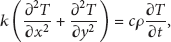
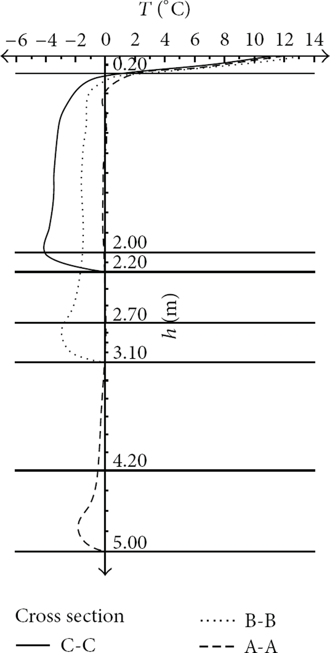
Mirambell and Aguado [35] expanded the finite difference method from one dimension to two dimensions in order to determine the time-dependent vertical and transverse temperature differences within the cross section of concrete bridges. The same assumptions about environment condition used by Elbadry and Ghali [23] were adopted in this study. The main objective of this study is investigating the influence of the cross section geometry of concrete box girder bridges on their thermal distribution. The results indicated that the maximum vertical temperature difference and the daily range of effective temperature of the cross section decrease with an increase in the superstructure depth, as shown in Figure 2. In the figure, the depths of sections A-A, B-B, and C-C are 2.2 m, 3.1 m, and 5.0 m, respectively. The outcome of the study also indicated that the ranges of the daily variation of the vertical temperature difference and the effective temperature are higher in the unicellular cross section than those in multicellular cross section. In concrete box girder bridges with variable bending stiffnesses along the longitudinal axis of the bridge, the cross section subjected to the greatest vertical temperature difference and to the greatest temperature difference between the external air and the air enclosed in the cells is the midspan section, while the cross sections of the intermediate supports are subjected to the greatest transverse temperature differences. Comparing the geometrical parameters, it was found that the superstructure depth and the ratio between the deck's upper and bottom slab width are those with the greatest influence on the temperature distributions of concrete box girder bridges. It should be noted that this investigation pointed out the transverse temperature difference caused by the difference of temperature between the external air and the air enclosed within the cells which is significant and should be considered in design when the superstructure depth is large, which was rarely mentioned before. According to the study, the daily evolution of transverse temperature difference at the three cross sections is displayed in Figure 3.

Figure 2

Temperature distributions along the depth of cross section [35].

Figure 3

Daily evolution of transverse temperature difference at the three cross sections [35].

In the following ten years, the researches of temperature distribution in bridge by finite difference method are seldom. Until 2007, Riding et al. [36] proposed a mass concrete temperature prediction model employing the finite difference method to characterize the heat transfer at the top and side surfaces of concrete members. The model includes solar radiation, atmospheric radiation, ground surface radiation, radiation exchange with formwork bracing, and irradiation. The effects of free convection, forced convection, and surface roughness were also characterized in the model. The predicted temperatures were compared with concrete temperature data collected from 12 concrete members of varying geometry, formwork, location, construction methods, and materials. The results showed that the finite difference heat transfer model can accurately estimate the near-surface concrete temperatures, the maximum temperature, and maximum temperature difference of the 12 concrete members.

3.2. Finite Element Method

Apart from the finite difference method, another particular class of numerical techniques for the approximate solution of partial differential equations is the finite element method, which originated from the need to solve complex elasticity and structural analysis problems in civil and aeronautical engineering. This method was proposed in a seminal work of Richard Courant in 1943 [37] and obtained its real impetus from the contributions of many forerunners, like Argyris, Clough, Zienkiewicz, and Richard Gallagher, in the 1960s and 70s. Now, finite element methods have been developed into one of the most general and powerful class of techniques for the numerical solution of partial differential equations and are widely used in structure design and analysis.

By assuming that the thermal variation in the longitudinal direction of the bridge and the transverse heat flow are insignificant, Priestley [38] conducted a one-dimensional finite element analyse and proposed a most widely accepted thermal gradient model of box girder concrete bridge. The model describes the thermal gradient by fifth-order curve and has been validated for sections with relatively small depths by several theoretical and experimental programs. This model was then adopted by bridge design code in New Zealand.

In 1978, Emanuel and Hulsey [39] provided a finite element model to predict the vertical temperature distribution through the cross section of a composite bridge beam at different hours of day and night from weather data by assuming concrete as homogeneous and isotropic. They showed how the ambient conditions influence the temperature distribution in a composite section. Afterward, Berwanger [40] established an accurate two-dimensional finite element procedure for predicting transient temperatures in composite slab-steel beam highway bridges. A linear temperature rectangular finite element is used. The numerical integration for successive time increments was carried out using the Crank-Nicolson approximation. Statistical analyses indicated a better than 0.99 probability of correlation between the predicted and measured temperatures.

Elbadry and Ghali [23] proposed a two-dimensional finite element method to predict the time-dependent nonlinear temperature distribution over concrete bridge cross sections of arbitrary geometry and orientation. By using the bilinear quadrilateral interior elements to simulate the inner body and linear one-dimensional fictitious elements to represent the boundaries, the finite element formulations were established. A series of transient finite element analyses were performed to study the influences of various parameters including bridge axis orientation, ambient temperature extremes, wind speed, surface cover, and section shape on the temperature distribution of concrete bridges of various cross section types. The outcome of the study indicates that the temperature gradient is in general greater in summer than it is in spring or winter. The temperature gradient increases with increasing the daily range of the ambient air temperature. Higher wind speed tends to bring the temperature of the bridge surfaces closer to that of the ambient air. The presence of asphalt overlay on the concrete deck results in an increase in the top surface temperature, and snow reduces each of these variables. Bridges of the same depth but with different cross section shapes have almost the same temperature distribution, and the temperature distribution varies considerably with the section depth being verified.

Based on a finite element program ADINAT, a two-dimensional analysis was performed by Fu et al. [14] to study the thermal behavior of three types of composite bridge structures subjected to solar radiation, namely, a plate-girder, a single-cell box, and a two-cell box girder concrete-steel composite bridge. A series of transient temperature distributions for a few selected temperature cases corresponding to a given geographic location and assumed environmental conditions was computed. The results of this study confirmed that a steady-state thermal condition never exists within a bridge structure. Meaningful conclusions were drawn in this research including the most influential variable on the temperature distribution within a bridge deck which appears to be the slab overhang-to-depth ratio; the effects of heating of air inside an enclosed box should be included in predicting the temperature distribution for box girder bridges; the convection constant, that is, the cooling or heating produced by the wind, substantially affects the temperature distribution when the bridge is being heated by solar radiation; and daily air temperature extremes have a marked influence on the thermal distribution of a composite bridge.

Moorty and Roeder [41] conducted a two-dimensional analysis for a typical bridge with concrete box girder, concrete T-beam, and steel girder with a composite deck using the finite element program ANSYS. The isoparametric quadrilateral thermal shell elements were used to model the deck, concrete T-beams, and box girders. Two-dimensional conducting bar elements were used to model the steel girders. The convection boundary conditions were achieved using convection links. The analysis was conducted for four days in order to eliminate the effect of the assumed initial conditions and suggested that concrete bridges sometimes are designed for smaller temperature ranges than expected values in practice, and steel bridges with composite concrete decks sometimes are designed for larger temperature ranges than expected values at many locations in the United States. Subsequently, Branco and Mendes [42] provided a numerical technique for the resolution of the Fourier heat transfer equation based on the two-dimensional finite element method. The results obtained with this technique had been demonstrated by several cases with experimental measurements. To come up with design thermal linear gradients, a parametric study had been developed for three types of typical deck cross sections: slab deck, T-beam deck, and box girders. The results formed two vertical temperature differences for two solar radiation conditions, and the design temperature differences for other situations can be calculated from the reference ones through the adjustive coefficients estimated by the parametric study. Furthermore, it was found that temperature differences occur among the deck, towers, and cables during the day in cable-stayed bridges due to the different orientation of the structural elements to the sun. In long-span cantilever bridges, the variation of the cross section leads to different design thermal gradients along the span.

Early researches concentrate on concrete bridges and composite bridges; with the wide use of steel in bridges all over the world, the study on thermal load in steel bridges was also implemented. Tong et al. [43] developed a numerical two-dimensional heat transfer model for the analysis of temperature distribution in steel bridges. By assuming that the longitudinal heat flow in a prismatic deck can be neglected under normal circumstances and there is negligible temperature gradient across the thickness of steel plates because of the high thermal conductivity and small thickness of steel plates, the matrix “equilibrium” equation for steel plate was established, and then the temperature distribution of the bridge had been obtained by carrying-out time marching following the standard finite element procedure. The proposed approach was validated by two scaled steel box models. Sensitivity analysis showed that the top film coefficient and absorptivity have significant effect on temperature distribution. In addition, a least square method was suggested for backfiguring best values for the input parameters, if they are not available. Then, they integrated a statistical model, which was established by the numerical integration technique suggested by Evans [34] and subsequently modified by Ho and Liu [33] into this finite element model and developed a statistical approach to determine site-specific temperature profiles for code documents where the requisite climatic information for a particular geographic location is available [44]. Based on the method, some fifth-order design temperature profiles had been developed for both open and closed steel sections in tropical region, with adjustments for various thicknesses of bituminous surfacing, as shown in Figure 4. The proposed method avoids very lengthy calculations and facilitates the development of site-specific temperature profiles for code documents if the field measurement temperatures are unavailable, and it can also be applied to create zoning maps for temperature loading for large countries like the United States where there are great climatic differences.

Figure 4

Design temperature profiles for various bitumen thicknesses (b.t.) for 50-year return period [44].

In the 21st century, the commercial finite element software has been developed rapidly. The powerful processing capability makes the temperature distribution analysis of bridges with complex geometric configuration competent. Backer et al. [45] established a detailed finite element model of a steel box girder within the Vilvoorde Viaduct, including stiffeners, diaphragms, and wearing courses, by using commercial finite element software in order to reach a fundamental insight into the temperature distribution of the cross section with orthotropic stiffeners, subjected to a variable thermal load. All thermal fluxes within this system were modeled including solar radiation, radiation with the environment, mutual radiation, and convective airflow, which allowed verification of the temperature variations in the steel box during a 24-hour cycle as well as during a longer period. The finite element models developed for this research had validated the possibility to model mutual radiation between the different objects within the model and the surrounding environment. The simulated results were demonstrated by the field measurement data. The temperature distribution in such a steel box girder on a sunny summer day at noon is plotted in Figure 5. The asphalt layer is not displayed in this figure. It is immediately obvious that an important temperature difference can arise between the upper and lower part of the box girder. For this specific example, the temperature difference rises to a value of more than 40°C. Studying the top view of the deck plate of the bridge, as shown in the right side of Figure 5, the influence of the underlying structure and the diaphragms is quite obvious. Kim et al. [25] proposed a method to predict the 3-dimensional temperature distribution of curved steel box girder bridges using a theoretical solar radiation energy equation together with a commercial FEM program. The diverse range of bridges directions, radii, span lengths, and bearing setup directions was taken into consideration. It was strongly suggested that the nonuniform temperature distribution brought about by solar radiation should be considered in the design of curved bridges.

Figure 5

Temperature distribution in the steel part of a typical box girder bridge (unit: °C) [45].

Xia et al. [46], for the first time, investigated the temperature distribution in a long-span suspension bridge—the 2132-m-long Tsing Ma Bridge—through finite element analysis. With appropriate assumptions, the bridge was divided into deck plate, section frame, and bridge tower, as shown in Figure 6. Fine finite element model of each component was constructed to facilitate thermal analysis. With ambient temperature measurements and a solar radiation model, the time-dependent temperature distribution within each of these components was calculated through transient heat transfer analysis. The numerical results were verified by comparing them with field monitoring data on temperature distributions and variation at different times and in different seasons, which provide thermal loads for thermal effect analysis of long-span suspension bridge.

Figure 6

Finite element models of bridge components for thermal analysis [46].

In addition, Lee [47] performed a 2D heat-transfer analysis based on finite element method. The model was firstly validated and then used to determine the seasonal temperature gradients in four standard PCI girder sections at eight cities in the United States. The proposed vertical thermal gradient and transverse thermal gradients with respect to the locations across the top flange, the web, and the bottom flange of prestressed concrete bridge girders were shown in Figures 7 and 8, respectively. On the basis of the numerical model and the extreme environmental conditions, the maximum vertical temperature differentials were found in the summer in an east-west orientation, and the maximum transverse temperature differentials were found in the winter in an east-west orientation. The differences in the maximum vertical and transverse temperature differentials between the exterior and interior girders were negligible during construction, prior to the placement of concrete decks. The results show that, among the four AASHTO-PCI sections, the deeper and wider sections of Type-V and BT-63 girders exhibited the largest vertical and transverse temperature differentials.

Figure 7

Vertical thermal gradient of prestressed concrete bridge girders [47].

Figure 8

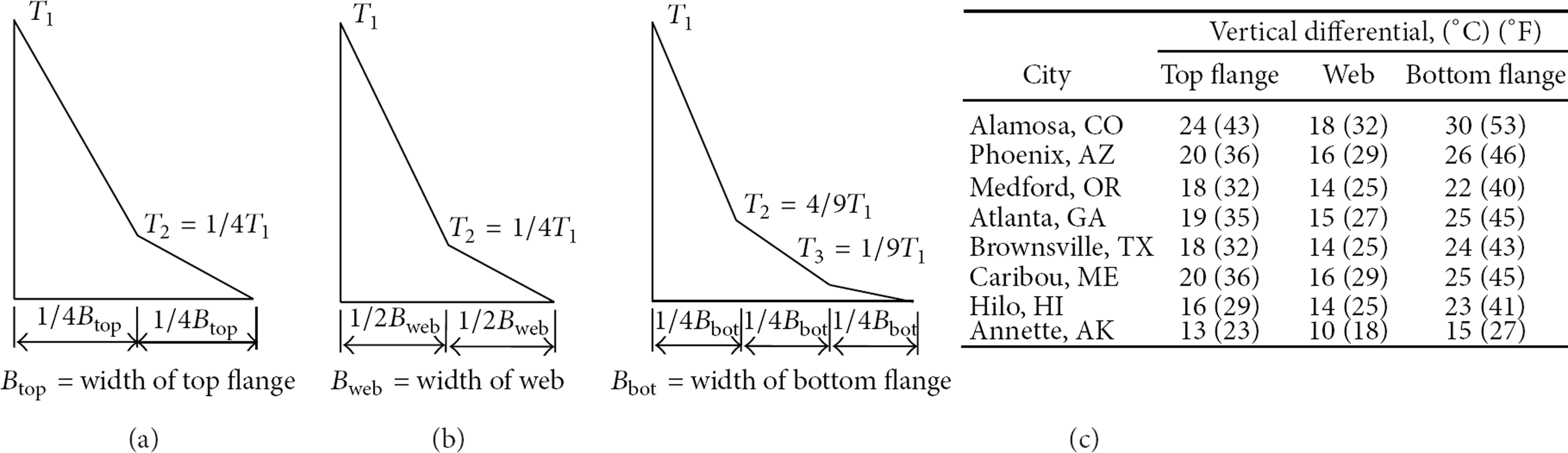
Transverse thermal gradients of prestressed concrete bridge girders: (a) top flange, (b) web, and (c) bottom flange [47].

Numerical analysis provides a perfect approach to predict the thermal load in bridge with different boundary conditions and makes it possible to perform extensive study on the influence of environment conditions, geometrical configuration, and material property. It is useful for a thorough understanding of the temperature behavior of various types of bridges and gives basic concept for thermal stresses calculation in bridge design. However, numerical approaches are input parameters dependent. The simulated results rely on the values of input parameters. As some input parameters depend greatly on environmental factors and change with time, the predicted values for these parameters may not match perfectly with the practical ones. As a result, the calculated thermal load may deviate from the real case. Moreover, it is impossible to simulate the thermal load for several months or several years. Field measurement, which can provide practical thermal load in bridge for a long time and is immune to input parameters, is a powerful alternative.

4. Field Measurement

The thermal load in bridge is affected by air temperature, wind, humidity, intensity of solar radiation, material type, and so forth, which make it not easy to be modeled by theoretical or numerical approach. Field measurement that monitored the temperature in bridge by temperature sensors installed on it can give the most objective data of temperature subjected to real climatic change. It also provides the criterion for demonstrating the validation of theoretical or numerical results. With the development of sensor and computer technology, field measurements of thermal loads in bridges have been carried out extensively in various bridges. In particular, recent advances in sensing, data acquisition, computing, communication, and data and information management, have greatly promoted the applications of structural health monitoring (SHM) technology in bridge structures [48, 49]. Successful implementation and operation of SHM systems on bridges have been widely reported in different countries. Almost all SHM systems include temperature monitoring subsystem, for example, a total number of 83 sensors were installed on the Ting Kau Bridge to monitor the temperature of air, concrete, steel, and asphalt, and more than 200 temperature sensors were configured on the Tsing Ma Bridge and the Kap Shui Mun Bridge [50, 51]. The temperatures of bridge components are measured continuously for a long-term period, which provide valuable data for study of temperature distribution in bridge and allow carrying out prediction of the extreme thermal loads with a certain return period.

4.1. Temperature Sensor

The temperature sensor is the key component when implementing field measurement of thermal load in bridge. There are many types of temperature sensors that are capable of measuring temperature such as thermocouple, platinum resistance thermometer, fiber Bragg grating (FBG) temperature sensor, and wireless temperature sensor.

The thermocouple is the most common one. A thermocouple consists of two dissimilar conductors in contact, which produces a voltage when heated. The voltage produced is dependent on the difference of temperature of the junction to other parts of the circuit. Commercial thermocouples are inexpensive and interchangeable and can measure a wide range of temperatures. In contrast to most of other methods of temperature measurement, thermocouples are self-powered and require no external form of excitation. The main limitation with thermocouples is accuracy; system errors of less than one degree Celsius (°C) can be difficult to achieve.

Platinum resistance thermometer is another type of electrical temperature sensor used for field measurement of thermal load in bridge. It determines the temperature by measuring the electrical resistance of a piece of pure platinum wire. By using the characteristic that the electrical resistance of platinum increases approximately linearly with absolute temperature, the resistance of a wire of platinum is measured by passing a current through it, and the reading is converted to temperature using a calibration equation. With proper design, the resolution of less than 0.1°C can be obtained.

For the outstanding properties of small size, high sensitivity, insensitivity to electric or magnetic inference, localized strain measurement ability, and multiplexing capability, the FBG temperature sensor is widely used for temperature test [52–54]. The FBG is an optical fiber which is formed by exposure to a fringe of UV light. Only the specified Bragg wavelength related to its grating period is reflected for an input light wave from a broadband source. The temperature change causes shift of Bragg wavelength. Then the temperature variation can be tested by recording the change of Bragg wavelength. The resolution of FBG temperature sensor is less than 0.1°C.

The wireless sensor network is a promising technology for structural test. By many attractive features of wireless communication, onboard computation, relatively low cost, and small size, the shift of field temperature measurement away from traditional wired sensor toward the use of wireless sensor has been motivated. In general, the sensing element of wireless temperature sensor does not have much difference with wired temperature sensor, and the biggest difference lies in the fact that the collected temperatures are transmitted to the base station by wireless sensor network. Now, the wireless temperature sensor has been applied in many bridges [55, 56].

Furthermore, temperature sensing component is frequently integrated in those sensors used test other physical parameters, for examples, strain sensor [57], displacement sensor [58], and wireless acceleration sensor [59]. It is worth to say that there are a large number of types of temperature sensors. Only four typical types of sensors are introduced here for the limited space. What is more, the contributions of researchers make the novel temperature sensors emerge every year.

4.2. Data Processing Methodology

For both daily air temperature and daily global solar radiation varying in a random manner, rational conclusions about thermal load in bridge can only be obtained by statistical approach [33]. So, generally, the processing of field measurement data can be divided into four stages including data preprocessing, trend analysis, statistical analysis, and extreme value analysis (EVA). Those stages are not indispensable, and some procedures may be omitted on specific occasion.

In field measurement, it is inevitable that the test data is disturbed by noise and malfunctions of data acquisition system. So there are some unreasonable data with abnormal magnitude existence in the records. Prior to extract thermal load, those problematic records should be identified. Xu et al. [13] suggested three criteria to identify the abnormal data. The first one is that the difference between the hourly maximum and minimum values is greater than a problem specific limitation. The second one is that the standard deviation of measured hourly records is equal to zero. And the third one is the hourly mean value of temperature that is smaller than a threshold value of minimum temperature. One way to deal with those problematic records is elimination. The problematic data are eliminated directly and left blank in the data series. And another way is repair. The problematic samples are repaired by either interpolation between normal records within the sample or replacement by other samples with similar recordings [6].

Trend analysis is a common data processing method. For the slow change of temperature, the hourly, daily, or monthly average temperatures are calculated firstly. The time histories of those mean values are then plotted in figures. The trend of temperature changing with time can be investigated. The data measured in different locations can also be compared.

Statistical analysis is using the probability density function (PDF) to describe the frequency distributions of different temperatures. The normal distribution, logarithmic normal distribution, and Weibull distribution are usually adopted. For estimating the PDF of random temperatures, two statistical methods, that is, nonlinear regression and hypothesis testing, are used.

EVA is a special field that concentrates on the behaviour of the extreme observations instead of the complete sample population, which allows generalization of return periods of extreme events by extrapolating from the available observations and has been widely used in various engineering fields where extreme values are of importance [60, 61]. The results of EVA can provide reference values of extreme thermal loads for bridges design.

4.3. Concrete Bridge

From 1982 to 1984, Ho et al. [62] carried out field measurements on a prestressed concrete bridge in Hong Kong. A total of 72 thermal sensors had been installed in the multicellular and the solid portion of a prestressed concrete bridge deck of depth 1.4 m. Temperature readings were taken at hourly intervals, and the data were stored on cassette tapes. The measuring system was designed for a temperature range of 0°C–75°C and a system accuracy of ±0.5°C. The results were used to verify the proposed one-dimensional finite difference model by statistical manner. In 1984, McClure et al. [21] studied the longitudinal, horizontal, and vertical temperature variations in a posttensioned segmental concrete box girder bridge from the measured data obtained by thermocouples. Based on a regression analysis, it was concluded that there was no significant longitudinal temperature variation. Furthermore, the results showed that there was little transverse temperature variation. These results confirmed earlier assumptions that the three-dimensional heat-flow problem in a bridge can be reduced essentially to a one-dimensional state comprising of a vertical temperature variation through the section depth of the bridge.

In 1998, large amount of thermocouples was instrumented on the North Halawa Valley Viaduct in Hawaii by Shushkewich and readings were been taken over a five-year period [63]. A simplification to the computation procedure for the analysis of nonlinear thermal gradient was proposed. The processing of the data revealed that the results correlate extremely well with the positive and negative thermal gradients in proposed revision to an AASHTO specification [64]. The reduction of the negative thermal gradient by 40% and the maintaining of the positive thermal gradient in the new edition were validated duly.

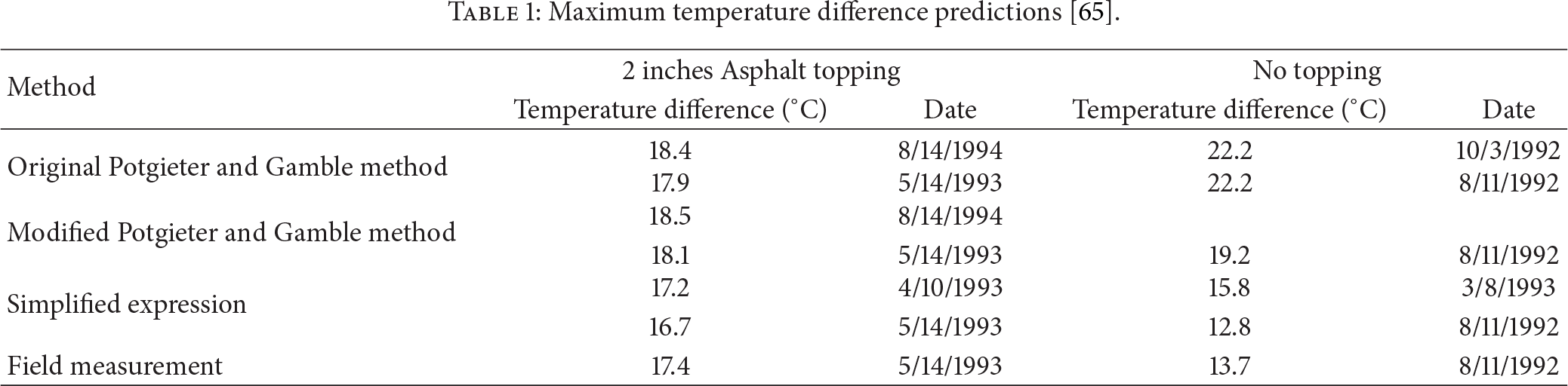
Supported by the San Antonio “Y” project, a segmental concrete box girder bridge was instrumented with several thermocouples through the depth, which recorded temperatures every half hour for 2 1/2 years [65]. The maximum recorded positive and negative thermal differentials were investigated by Roberts-Wollman, and it was reported that both the typical positive gradient curve and negative gradient curve can be approximated by a fifth-order parabola with different points of zero temperature difference. When comparing to design recommendations, the conservative values of the AASHTO recommendations were found out for the San Antonio area. A simplified expression was sought to calculate the temperature difference only in terms of the solar radiation and the difference between daily high temperature and 3-day average temperature. The predicted maximum temperature differences were compared with the results calculated by original Potgieter and Gamble method [31], modified Potgieter and Gamble method [31], and field measurement as shown in Table 1. It can be seen that all methods are within 1°C of predicting the maximum temperature difference for the 50 mm asphalt condition. For the no-topping condition, the Potgieter and Gamble method overestimates the magnitude of the difference. And the simplified expression better predicts the magnitudes for the no-topping case.

Table 1

Maximum temperature difference predictions [65].

Method	2 inches Asphalt topping		No topping
Method	Temperature difference (°C)	Date	Temperature difference (°C)	Date
Original Potgieter and Gamble method	18.4	8/14/1994	22.2	10/3/1992
Original Potgieter and Gamble method	17.9	5/14/1993	22.2	8/11/1992
Modified Potgieter and Gamble method	18.5	8/14/1994
Modified Potgieter and Gamble method	18.1	5/14/1993	19.2	8/11/1992
Simplified expression	17.2	4/10/1993	15.8	3/8/1993
Simplified expression	16.7	5/14/1993	12.8	8/11/1992
Field measurement	17.4	5/14/1993	13.7	8/11/1992

A renovated continuous three-span curved post-tensioned concrete bridge with a five-cell curved prismatic box girder had been monitored by twelve thermocouples for at least one year [16]. The temperature data were collected at fifteen-minute intervals. The data were evaluated by Fu et al. and showed that there are large changes in the ambient temperature and mean temperature within the bridge during the year; however, there is very little change in the magnitude of the differential temperatures through the bridge during the year. Review of the temperature data for the bridge and the ambient temperature data indicated there is a time lag of approximately 10.6 hours between the peak of ambient temperature and the peaks of the measured bridge interior surface temperatures. Li et al. [6] monitored the Confederation Bridge, which is the world's longest bridge built over ice-covered water, by 142 thermocouples. The temperatures that were recorded at hourly intervals from 1998 to 2000 were analyzed. The data were firstly carefully screened to identify the outliers and unrealistic values and spatially reduced to a set of thermal variables including average, differential, and residual temperatures. The measurements of the south and north haunches and at the top of the webs in the deepest section and in the midspan section of the bridge were plotted in Figure 9 together with curves produced by $T = T_{top} {[(1200 - y) / 1200]}^{n}$ , with $n = 3$ , 4, and 5. y denotes the distance from top surface. It was observed that temperatures in the deepest section fit the cubic curve ( $n = 3$ ) better than the 5th-power curve ( $n = 5$ ) of Priestley, and the 5th-power curve follows the observations of midspan section more closely. EVA showed that all the thermal variables follow a Gumbel distribution, and the Canadian highway bridge design code gives a fairly good estimation for average temperatures but underestimates positive linear differential temperatures by 20% for the Confederation Bridge. Those findings improve our knowledge of extreme thermal behaviour of concrete bridges and are helpful for future development of thermal design criteria in bridge codes.

Figure 9

Fit of the temperature distribution to $T = T_{top} {[(1200 - y) / 1200]}^{n}$ [6].

Kulprapha and Warnitchai [66] equipped several temperature sensors on a continuous prestressed concrete bridge model with an I-shaped cross section. It was found that the temperature distribution is approximately uniform and stable from around midnight until early morning. From early morning until early afternoon, the temperatures at the deck and at other levels close to the deck rise at a much higher rate than those at the lower levels and the soffit. The maximum difference between deck and soffit during the day is about 20°C. From late afternoon to early night, the temperatures at the deck and other levels close to the deck fall at a much higher rate than those at the lower levels and the soffit. The maximum recorded deck and soffit temperatures are 56.3°C and 40.5°C, respectively. In addition, these measurement results confirmed that cross sectional temperature distribution is a function of only the height measured from the soffit. Lee [47] conducted measurements on a five-foot-long prestressed BT-63 girder from April 2009 to March 2010 in Atlanta, with the girder in an east-west orientation such that only the top surface and one side of the girder received direct solar radiation. Both the vertical temperature distribution and the transverse temperature distribution were measured. The daily maximum vertical temperature difference, as shown in Figure 10, was the largest in the summer and decreased from summer to winter. Unlike the vertical temperature difference, the maximum transverse temperature difference, as shown in Figure 11, was the largest in the late fall and winter as a result of higher solar radiation on the vertical surfaces of the girder facing the south.

Figure 10

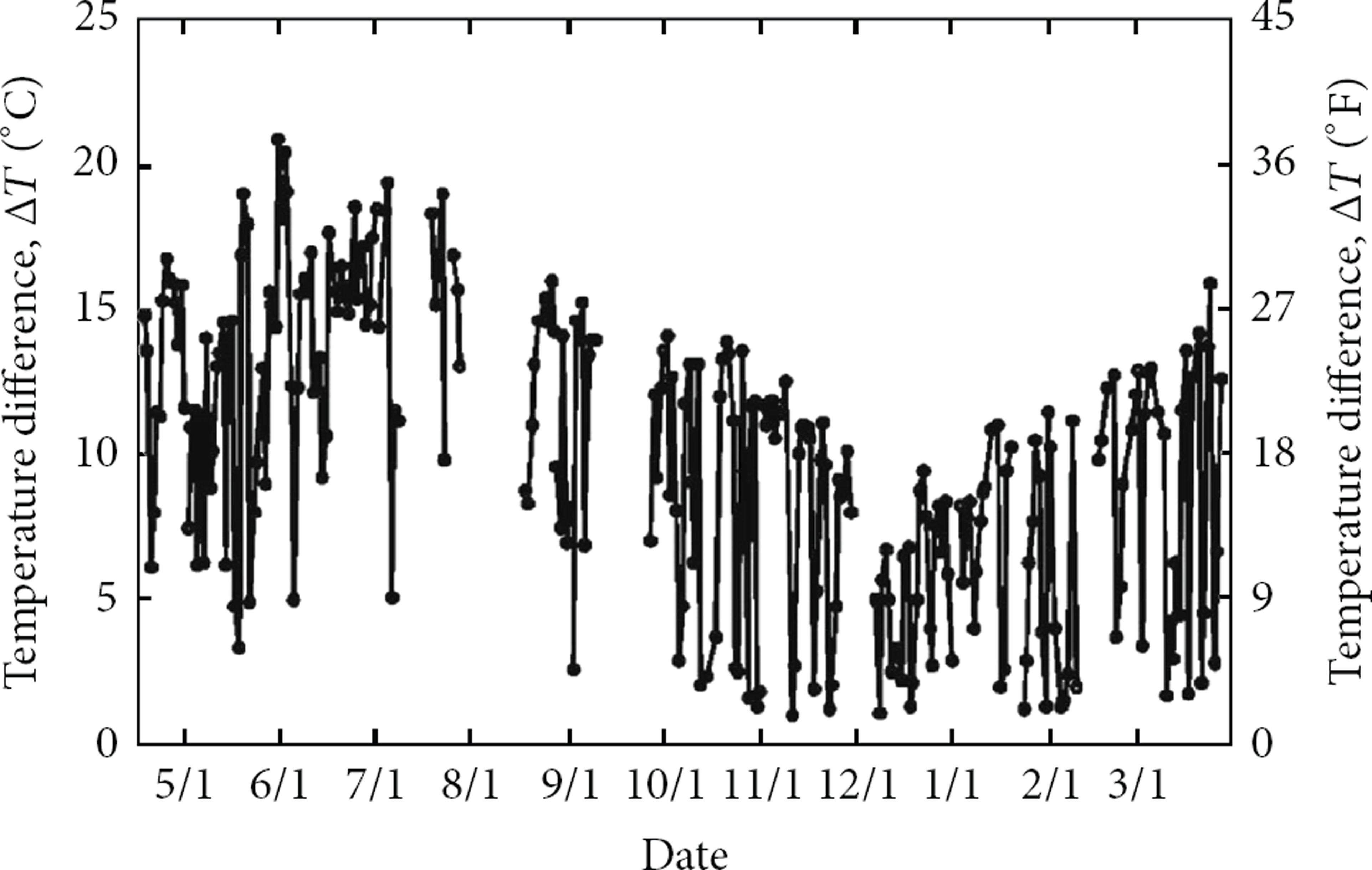
Daily vertical temperature difference along the depth of the girder [47].

Figure 11

Daily transverse temperature difference across the bottom flange [47].

4.4. Steel-Concrete Composite Bridge

The steel-concrete composite bridge is composed of steel beam and concrete slab. The different heat transfer coefficients of steel and concrete make a nonlinear thermal gradient along the vertical axis of the cross section. As a result, the model of thermal load is different from that in homogeneous material. In composite bridge, the thermal stresses were found to be comparable to the dead load and live load stresses. So the thermal load in steel-concrete composite bridge is particularly important.

In 1957, Naruoka et al. [67] carried out temperature tests on the interior of the Shigita Bridge in Japan, which is a simply supported bridge with a reinforced deck slab-on-steel girders. A typical vertical temperature distribution in the month of July was obtained. The results of the tests showed that the distribution is almost constant in the steel girder and fairly linear in the concrete deck slab. The maximum differential temperature between the top and bottom of the concrete deck slab is about 22°C. It was also observed that the thermal gradient in the blacktopping is quite steep.

In 1965, Zuk [68] found that the temperature differentials between the top and bottom of the concrete deck slab can be as high as 22°C during the summer and as low as −6°C in the winter from field measurements on six simply supported composite bridges. In another study, he obtained the vertical temperature distribution from field data in a composite bridge over the Hardware River near Charlottesville, North Carolina [18]. The results revealed that the temperature differences between the top and bottom of the concrete deck slab ranged from 11°C to 19°C during the day and −2°C to 4°C during the night. The vertical temperature distribution was almost linear in the concrete deck slab with very small variation through the depth of the steel girder. So for all practical purposes, it can be considered to be uniform and equal to the ambient temperature gradient.

Based on a synthesis of several theoretical studies and experiments on prototype composite concrete slab-on-steel beam bridges conducted by Naruoka et al. [67], Zuk [18, 68], Berwanger [69], Emanuel and Hulsey [39], and so on, a simple but realistic vertical temperature distribution through the section depth is proposed by Kennedy and Soliman [70], as shown in Figure 12. The proposed distribution is linear through the depth of the slab and uniform through the depth of the steel beam. This distribution leads to simple formulas to estimate the thermal stresses in simple and continuous composite bridges.

Figure 12

Proposed linear-uniform vertical temperature distribution [70].

Au et al. [71] conducted a comprehensive investigation on the thermal behavior of bridges in Hong Kong with special emphasis on composite bridges. The outcome of the study demonstrated that the temperature distribution in bridge depends primarily on the solar radiation, ambient air temperature and wind speed in the vicinity. Apart from data of the meteorological factors, good estimates of the thermal properties of material and the file coefficients are necessary for the prediction of thermal load. A fifth-order equation of the design temperature profile for tropical regions was suggested, which is very similar to the one proposed by Priestley [72] for concrete box girders.

Im and Chang et al. [73] monitored a steel-concrete composite box girder bridge located at the south of Seoul by 30 copper-constant thermocouples over a 6-year period. The thermal load parameters including effective temperature, vertical temperature difference, and horizontal temperature difference were computed based on measured data. The hourly variation of the horizontal temperature differences revealed that the horizontal temperature differences are no longer negligible since they are of the same order of magnitude as the vertical temperature differences in the winter months. EVA indicated that all the thermal load parameters of hourly maximum and hourly minimum values obey the Gumbel distribution.

4.5. Steel Bridge

Because of the high thermal conductivity, steel adjusts its temperature many times faster than concrete, leading to a more rapid heat exchange between steel bridge and surrounding air. As a result, the thermal loads in steel bridges have much difference with that in concrete bridges.

Ni et al. [12] investigated one-year (the year of 1999) continuous measurement data recorded by a total of 83 temperature sensors, which had been installed at different locations of the Ting Kau Bridge in Hong Kong to measure (1) steel-girder temperature, (2) temperature inside concrete deck, (3) temperature in tower legs, (4) temperature in asphalt pavement, and (5) atmosphere temperature. It was observed that, in general, the temperatures in asphalt are the highest and the temperatures in atmosphere are the lowest. The temperatures measured at different locations, on the same cross section, attain their maxima almost at the same hour. The EVA was employed to estimate the extreme effective temperatures of bridge deck with a certain return period. The predicted maximum and minimum effective temperatures for a return period of 120 years are 36.9°C and −3.6°C, respectively, which agree well with the design values. De Backer et al. [45] implemented an autonomous monitoring system for temperatures in the southern box girder of the Vilvoorde Viaduct during the spring months of 2008. The results illustrated the validity of the claim that a second internal heating takes place, due to mutual radiation and heat conduction, after the solar radiation has reached its peak.

Xu et al. [13] installed a total number of 109 sensors to implement temperature measurement on the Tsing Ma Bridge. The temperatures of bridge cross section, cable, and air were monitored. Subsequently, the temperature monitoring data from 1997 to 2005 were evaluated. After the problematic data were eliminated, monthly statistics of effective deck temperature including mean, minimum, and maximum temperatures were computed. The results indicated that there is a clear and fairly stable cycle of ambient air temperature variation. The ambient air temperature reaches the lowest values normally in January every year, while the highest level is in July or August every year. The comparison of monthly effective deck temperature and ambient air temperature in 1999–2005 revealed that the effective bridge deck temperature has similar variation patterns to those of the ambient air temperature. The minimum effective temperature of bridge deck, main cable, and air is almost the same, while the maximum effective temperature of bridge deck is significantly higher. Cao et al. [74] studied the monitored temperatures including steel deck, stayed cables, and concrete tower of the Zhanjiang Bay Bridge, located in an inner gulf of South China, and found that the maximum temperature gradient in the steel girder was more than twice the original design value. The concrete temperature lagged significantly behind ambient air by 5-6 hours, and stayed cable temperatures were between those of ambient air and concrete.

The temperatures of the Runyang Suspension Bridge (RSB), with a span of 1490 m, were monitored since 2005 at a sample frequency of 1 Hz. The flat steel box girder was employed as the main girder in the bridge. Eight temperature sensors were embedded in one section and four cross sections were measured. Ding et al. [75] analyzed the representative data of 90 days that scatter to four seasons in one year uniformly. The results indicated that the temperatures in cross section have close relation with season. The time history of vertical temperature differences, horizontal temperature differential in bottom deck, and horizontal temperature differential in top deck were investigated, as shown in Figures 13, 14, and 15, respectively. It can be seen that the vertical temperature differences are mainly governed by solar radiation intensity, the horizontal temperature gradient in bottom deck is very small and can be neglected, and the horizontal temperature differentials in top deck have no relationship with time and cannot be ignored. Statistical results showed that the combined probability distribution model defined by the weighted sum of one Weibull distribution and one normal distribution can well describe the temperature differences. EVA results indicated that the daily extreme temperature differences in flat steel box girder cross section of the RSB followed the Weibull distribution, which have much difference with the general cases that the Gumbel distribution is obeying. According to correlation analysis, the critical temperature difference models in top plate of the flat steel box girder were proposed for thermal stresses calculation, as shown in Figure 16. The results provide a thorough understanding of thermal field in flat steel box girder bridges and have reference values for structural design and evaluation.

Figure 13

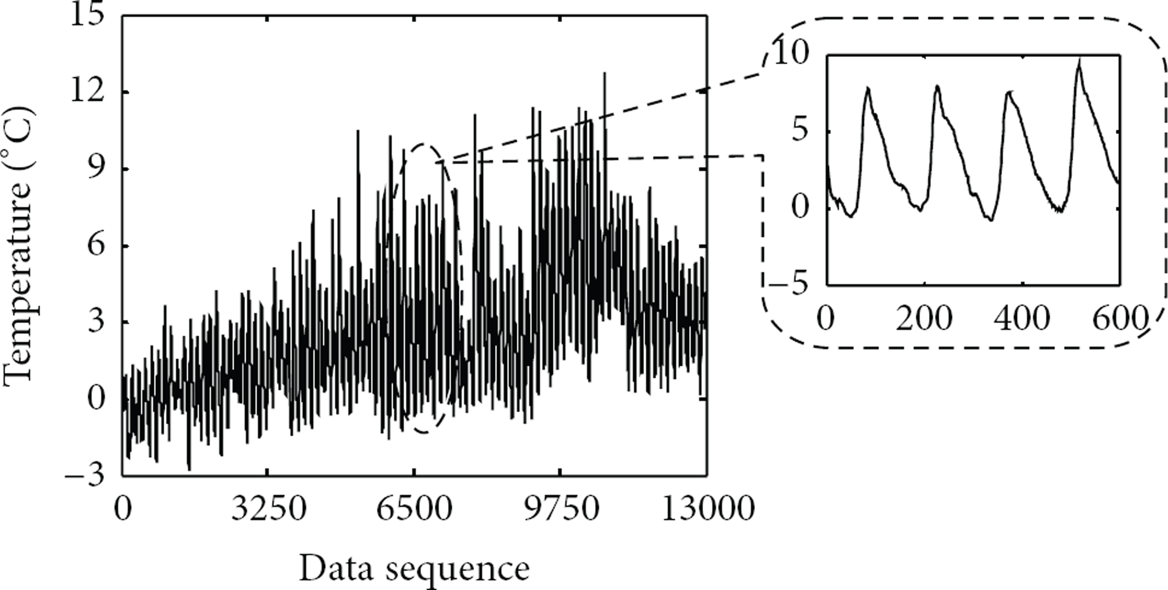
Time history of vertical temperature differential [75].

Figure 14

Time history of horizontal temperature differential in bottom deck [75].

Figure 15

Time history of horizontal temperature differential in top deck [75].

Figure 16

The critical temperature difference models in top plate [75].

5. Conclusions and Recommendations

The thermal load, which provides foundation for calculating thermal stresses, is one of the key parameters that affect the service ability of bridges. The research of thermal load in bridge by theoretical model, numerical analysis, and field measurement is progressed remarkably, and design guidance about thermal loads is also provided in specifications for general form of bridges. However, it is far from sufficient. At least, the following aspects need to be further attempted. (1)

The development of SHM technology makes performing automatic and real-time field measurement of temperature in bridge convenient. Although some bridges are monitored by temperature sensors, the measurement data are left unused, unlike the vibration and stress data that are investigated extensively. The effect of thermal load on the performance of bridges is not fully understood. So carrying out wide field measurements of temperature on different bridges in different regions should be encouraged, and particular emphasis should be placed on extracting thermal load models from field measurement data.

(2)

Nowadays, new concepts are employed in bridge design continuously. A lot of new bridges with complicated geometric configuration are constructed. At the same time, new materials are invented for bridge structures. The heat properties such as emissivity and absorptivity of those new materials are different from general cases. For those bridges, the existing design specifications are useless. In addition, the global climate has much difference with that in several decades years ago because of the development of industry and improvement of technology. So it is important to investigate thermal load in bridge with different schemes comprehensively.

(3)

Due to the complexity of heat transfer and heat exchange, it is difficult to predict the thermal load for all the cases and codify the results to simple rules and guidelines that accommodate climatic, geographic, geometric, and material variations. Definition of critical thermal loads varying from region to region, bridge to bridge, and section to section becomes significant. In addition, the modern transportation system had been extended to the extremely cold area and extremely hot area, but the research of thermal load on bridge in those regions has attracted little attention.

(4)

It is impossible that the temperature distribution in a bridge is described completely by limited data obtained by temperature sensors. So numerical models are powerful supplements. However, up to now, fine numerical models including all key components for simulating temperature distribution in large-scale bridges have not been developed. The intensity of solar radiation, the coupling effect of air temperature and wind speed, and the heat exchange between the surface and surrounding environment are not defined exactly. Moreover, the perfect transition from heat transfer analysis to thermal stresses analysis is not achieved.

(5)

Current specifications provide engineers with a temperature gradient across the depth of the cross section to predict the vertical thermal behavior of bridges based on one-dimensional heat flow. But the specifications do not provide any guidance for transverse temperature gradients that cause additional lateral deformations in the girders especially prior to the placement of the bridge decks during construction. Investigation results already demonstrated that those transverse temperature differences exist in many bridges and the values are greater than those of vertical temperature differences sometimes.

Footnotes

Acknowledgments

This research work was jointly supported by the Science Fund for Creative Research Groups of the NSFC (Grant no. 51121005), the National Natural Science Foundation of China (Grant nos. 51278104 and 51308186), the Natural Science Foundation of Jiangsu Province of China (Grant no. BK20130850), and the Research Fund of State Key Laboratory for Disaster Reduction in Civil Engineering (Grant no. SLDRCE12-MB-03).

References

Kareem

Aerodynamics and aeroelasticity of cable-supported bridges: identification of nonlinear features

Journal of Engineering Mechanics 2013 139 12 1886 1893

10.1061/(ASCE)EM.1943-7889.0000615

Magalhães

Cunha

Caetano

Vibration based structural health monitoring of an arch bridge: from automated OMA to damage detection

Mechanical Systems and Signal Processing 2012 28 supplement 1 212 228

2-s2.0-84857358404

10.1016/j.ymssp.2011.06.011

Johansson

Pacoste

Karoumi

Closed-form solution for the mode superposition analysis of the vibration in multi-span beam bridges caused by concentrated moving loads

Computers & Structures 2013 119 85 94

Jalali

R. S.

Bahari Jokandan

Trifunac

M. D.

Earthquake response of a three-span, simply supported bridge to near-field pulse and permanent-displacement step

Soil Dynamics and Earthquake Engineering 2012 43 380 397

Miyata

Yamada

Katsuchi

Kitagawa

Full-scale measurement of Akashi-Kaikyo Bridge during typhoon

Journal of Wind Engineering and Industrial Aerodynamics 2002 90 12–15 1517 1527

2-s2.0-0036905359

10.1016/S0167-6105(02)00267-2

Maes

M. A.

Dilger

W. H.

Thermal design criteria for deep prestressed concrete girders based on data from confederation bridge

Canadian Journal of Civil Engineering 2004 31 5 813 825

2-s2.0-10944236890

10.1139/L04-041

A. Q.

Miao

C. Q.

Health Monitoring of Bridge Structures 2009

Beijing, China

China Communications Press

Sohn

Dzwonczyk

Straser

E. G.

Kiremidjian

A. S.

Law

Meng

An experimental study of temperature effect on modal parameters of the Alamosa Canyon Bridge

Earthquake Engineering and Structural Dynamics 1999 28 7-8 879 897

2-s2.0-0032833429

Xia

Chen

Weng

Y. Q.

Y. L.

Temperature effect on vibration properties of civil structures: a literature review and case studies

Journal of Civil Structural Health Monitoring 2012 2 1 29 46

10.

Liu

DeWolf

J. T.

Effect of temperature on modal variability of a curved concrete bridge under ambient loads

Journal of Structural Engineering 2007 133 12 1742 1751

2-s2.0-36249020825

10.1061/(ASCE)0733-9445(2007)133:12(1742)

11.

Z.-D.

Simulation of the effect of temperature variation on damage detection in a long-span cable-stayed bridge

Structural Health Monitoring 2007 6 3 177 189

2-s2.0-34548303256

10.1177/1475921707081107

12.

Y. Q.

Hua

X. G.

Wong

K. Y.

J. M.

Assessment of bridge expansion joints using long-term displacement and temperature measurement

Journal of Performance of Constructed Facilities 2007 21 2 143 151

2-s2.0-33947382592

10.1061/(ASCE)0887-3828(2007)21:2(143)

13.

Y. L.

Chen

C. L.

Wong

K. Y.

Chan

W. Y.

Monitoring temperature effect on a long suspension bridge

Structural Control and Health Monitoring 2010 17 6 632 653

2-s2.0-84856326329

10.1002/stc.340

14.

H. C.

S. F.

Cheung

M. S.

Thermal behavior of composite bridges

Journal of Structural Engineering 1990 116 12 3302 3323

2-s2.0-0024919618

15.

Moorty

Roeder

C. W.

Thermal responses of skewed bridges. Developments in short and medium span bridge engineering

Proceedings of the 3rd International Conference on Short and Medium Span Bridges

1990

16.

DeWolf

J. T.

Effect of differential temperature on a curved post-tensioned concrete bridge

Advances in Structural Engineering 2004 7 5 385 397

2-s2.0-8344242860

10.1260/1369433042863251

17.

Maes

M. A.

Dilger

W. H.

Ballyk

P. D.

Extreme values of thermal loading parameters in concrete bridges

Canadian Journal of Civil Engineering 1992 19 6 935 946

18.

Zuk

Thermal behaviour of composite bridges-insulated and uninsulated

Highway Research Record 1965 76 231 253

19.

Saetta

Scotta

Vitaliani

Stress analysis of concrete structures subjected to variable thermal loads

Journal of Structural Engineering 1995 121 3 446 457

2-s2.0-0029271650

10.1061/(ASCE)0733-9445(1995)121:3(446)

20.

B. H.

Choi

S. C.

Cha

S. W.

Temperature and relative humidity analysis in early-age concrete decks of composite bridges

Measuring, Monitoring and Modeling Concrete Properties 2006

Dordrecht, The Netherlands

Springer

305 316

21.

McClure

R. M.

West

H. H.

Hoffman

P. C.

Observations from tests on a segmental bridge

Transportation Research Record 1984 2 60 67

22.

Duffie

J. A.

Beckman

W. A.

Solar Engineering of Thermal Processes 2013

Hoboken, NJ, USA

John Wiley & Sons

23.

Elbadry

M. M.

Ghali

Temperature variations in concrete bridges

Journal of Structural Engineering 1983 109 10 2355 2374

2-s2.0-0020840776

24.

Orgill

J. F.

Hollands

K. G. T.

Correlation equation for hourly diffuse radiation on a horizontal surface

Solar Energy 1977 19 4 357 359

2-s2.0-0017441648

25.

Kim

S.-H.

Cho

K.-I.

Won

J.-H.

Kim

J.-H.

A study on thermal behaviour of curved steel box girder bridges considering solar radiation

Archives of Civil and Mechanical Engineering 2009 9 3 59 76

2-s2.0-77950318663

26.

Dilger

W. H.

Ghali

Chan

Cheung

M. S.

Maes

M. A.

Temperature stresses in composite box girder bridges

Journal of Structural Engineering 1983 109 6 1460 1478

2-s2.0-0020766180

27.

Incropera

F. P.

Lavine

A. S.

DeWitt

D. P.

Fundamentals of Heat Transfer 2011

New York, NY, USA

John Wiley & Sons

28.

Emerson

The calculation of the distribution of temperature in bridges

TRRL Report 1973 LR 561

Department of the Environment

29.

Hunt

Cooke

Thermal calculations for bridge design

Journal of the Structural Division 1975 101 9 1763 1781

2-s2.0-0016556678

30.

Zichner

Thermal effects on concrete bridges

Bulletin d'Information 1982 154 291 314

31.

Potgieter

I. C.

Gamble

W. L.

Response of Highway Bridges to Nonlinear Temperature Distributions 1983

Urbana-Champaign, Ill, USA

University of Illinois

32.

Potgieter

I. C.

Gamble

W. L.

Nonlinear temperature distributions in bridges at different locations in the United States

PCI Journal 1989 34 4 80 103

33.

Liu

C.-H.

Extreme thermal loadings in highway bridges

Journal of Structural Engineering 1989 115 7 1681 1696

2-s2.0-0024703872

34.

Evans

D. H.

An Application of numerical integration techniclues to statistical toleraucing

Technometrics 1967 9 3 441 456

35.

Mirambell

Aguado

Temperature and stress distributions in concrete box girder bridges

Journal of Structural Engineering 1990 116 9 2388 2409

2-s2.0-0025491434

36.

Riding

K. A.

Poole

J. L.

Schindler

A. K.

Juenger

M. C. G.

Folliard

K. J.

Temperature boundary condition models for concrete bridge members

ACI Materials Journal 2007 104 4 379 387

2-s2.0-34547687457

37.

Brenner

S. C.

Scott

L. R.

The Mathematical Theory of Finite Element Methods 2008

New York, NY, USA

Springer

38.

Priestley

M. J. N.

Design thermal gradients for concrete bridges

New Zealand Engineering 1976 31 9 213 219

2-s2.0-0017001458

39.

Emanuel

J. H.

Hulsey

J. L.

Temperature distributions in composite bridges

Journal of the Structural Division 1978 104 1 65 78

2-s2.0-0017922557

40.

Berwanger

Transient thermal behavior of composite bridges

Journal of Structural Engineering 1983 109 10 2325 2339

2-s2.0-0020841559

41.

Moorty

Roeder

C. W.

Temperature-dependent bridge movements

Journal of Structural Engineering 1992 118 4 1090 1105

2-s2.0-0026854108

42.

Branco

F. A.

Mendes

P. A.

Thermal actions for concrete bridge design

Journal of Structural Engineering 1993 119 8 2313 2231

2-s2.0-0027641442

43.

Tong

Tham

L. G.

F. T. K.

Lee

P. K. K.

Numerical modelling for temperature distribution in steel bridges

Computers & Structures 2001 79 6 583 593

2-s2.0-0035254306

10.1016/S0045-7949(00)00161-9

44.

Tong

Tham

L. G.

F. T. K.

Extreme thermal loading on steel bridges in tropical region

Journal of Bridge Engineering 2002 7 6 357 366

2-s2.0-13844271559

10.1061/(ASCE)1084-0702(2002)7:6(357)

45.

de Backer

Outtier

van Bogaert

Numerical and experimental assessment of thermal stresses in steel box girders

Proceedings of the 11th Nordic Steel Construction Conference (NSCC '09)

2009

Swedish Institute of Steel Construction (SBI)

65 72

46.

Xia

Chen

Zhou

X.-Q.

Y.-L.

Field monitoring and numerical analysis of Tsing Ma Suspension Bridge temperature behavior

Structural Control and Health Monitoring 2013 20 4 560 575

2-s2.0-84855772492

10.1002/stc.515

47.

Lee

J. H.

Investigation of extreme environmental conditions and design thermal gradients during construction for prestressed concrete bridge girders

Journal of Bridge Engineering 2012 17 3 547 556

48.

Y. Q.

X. W.

J. M.

Monitoring-based fatigue reliability assessment of steel bridges: analytical model and application

Journal of Structural Engineering 2010 136 12 1563 1573

2-s2.0-81855161044

10.1061/(ASCE)ST.1943-541X.0000250

49.

Y. Q.

X. W.

J. M.

Modeling of stress spectrum using long-term monitoring data and finite mixture distributions

Journal of Engineering Mechanics 2012 138 2 175 183

2-s2.0-84857779090

10.1061/(ASCE)EM.1943-7889.0000313

50.

J. M.

Y. Q.

Technology developments in structural health monitoring of large-scale bridges

Engineering Structures 2005 27 12 1715 1725

2-s2.0-23844557791

10.1016/j.engstruct.2005.02.021

51.

Wong

K.-Y.

Instrumentation and health monitoring of cable-supported bridges

Structural Control and Health Monitoring 2004 11 2 91 124

2-s2.0-13244275053

10.1002/stc.33

52.

Ren

Sun

FBG sensors for on-line temperature measurements

5391

Smart Structures and Materials 2004: Sensors and Smart Structures Technologies for Civil, Mechanical, and Aerospace Systems

March 2004

94 99 Proceedings of SPIE

2-s2.0-10044262241

10.1117/12.538749

53.

H.-N.

Zhou

G.-D.

Ren

D.-S.

Strain transfer analysis of embedded fiber Bragg grating sensor under nonaxial stress

Optical Engineering 2007 46 5

2-s2.0-34447569511

10.1117/1.2739554

054402

54.

H.-N.

Zhou

G.-D.

Ren

D.-S.

Strain transfer coefficient analyses for embedded fiber bragg grating sensors in different host materials

Journal of Engineering Mechanics 2009 135 12 1343 1353

2-s2.0-70549089785

10.1061/(ASCE)0733-9399(2009)135:12(1343)

55.

Chae

M. J.

Yoo

H. S.

Kim

J. Y.

Cho

M. Y.

Development of a wireless sensor network system for suspension bridge health monitoring

Automation in Construction 2012 21 1 237 252

2-s2.0-81355147587

10.1016/j.autcon.2011.06.008

56.

Jang

Cho

Mechitov

Rice

J. A.

Sim

S.-H.

Jung

H.-J.

Yun

C.-B.

Spencer

B. F.

Jr. Agha

Structural health monitoring of a cable-stayed bridge using smart sensor technology: deployment and evaluation

Smart Structures and Systems 2010 6 5-6 439 459

2-s2.0-77953528539

57.

Guan

B.-O.

Tam

H.-Y.

Tao

X.-M.

Dong

X.-Y.

Simultaneous strain and temperature measurement using a superstructure fiber Bragg grating

IEEE Photonics Technology Letters 2000 12 6 675 677

2-s2.0-0034206535

10.1109/68.849081

58.

Tam

Chung

Demokan

M. S.

Fiber Bragg grating sensor for simultaneous measurement of displacement and temperature

Optics Letters 2000 25 16 1141 1143

2-s2.0-0001218623

59.

Kim

Pakzad

Culler

Demmel

Fenves

Glaser

Turon

Health monitoring of civil infrastructures using wireless sensor networks

Proceedings of the 6th IEEE International Symposium on Information Processing in Sensor Networks (IPSN '07)

April 2007

254 263

2-s2.0-35348857586

10.1145/1236360.1236395

60.

Castillo

Extreme Value Theory in Engineering 1988

New York, NY, USA

Academic Press

61.

Hadi

A. S.

Balakrishnan

Sarabia

J. M.

Extreme Value and Related Models with Applications in Engineering and Science 2005

Hoboken, NJ, USA

John Wiley & Sons

62.

Y. P.

Cornish

L. S.

Currie

L. G.

Temperature measurements in Castle Peak/Texaco Road flyover

Hong Kong Engineer 1984 12 9 29 33

2-s2.0-0021484372

63.

Shushkewich

K. W.

Design of segmental bridges for thermal gradient

PCI Journal 1998 43 4 120 137

2-s2.0-0032118485

64.

AASHTO Guide Specifications for Design and Construction of Segmental Concrete Bridges 1999 2nd

Washington, DC, USA

American Association of State Highway and Transportation Officials

65.

Roberts-Wollman

C. L.

Breen

J. E.

Cawrse

Measurements of thermal gradients and their effects on segmental concrete bridge

Journal of Bridge Engineering 2002 7 3 166 174

2-s2.0-10944259435

10.1061/(ASCE)1084-0702(2002)7:3(166)

66.

Kulprapha

Warnitchai

Structural health monitoring of continuous prestressed concrete bridges using ambient thermal responses

Engineering Structures 2012 40 4 20 38

2-s2.0-84858715652

10.1016/j.engstruct.2012.02.001

67.

Naruoka

Hirai

Yamaguti

The measurement of the temperature of the interior of the reinforced concrete slab of the shigita bridge and presumption of the thermal stress

Proceedings of the Symposium on the Stress Measurements for Bridges and Structures

1956

Tokyo, Japan

Japan Society for the Promotion of Science

68.

Zuk

Simplified Design Check of Thermal Stresses in Composite Highway Bridges 1965 Highway Research Record, no. 103

69.

Berwanger

The Modulus of Concrete and the Coefficient of Expansion of Concrete and Reinforced Concrete at below Normal Temperatures 1971 25

ACI Special Publication

70.

Kennedy

J. B.

Soliman

M. H.

Temperature distribution in composite bridges

Journal of Structural Engineering 1987 113 3 475 482

2-s2.0-0023306019

71.

F. T. K.

Cheung

S. K.

Tham

L. G.

Design thermal loading for composite bridges in tropical region

Steel & Composite Structures 2002 2 6 441 460

72.

Priestley

M. J. N.

Design of concrete bridges for temperature gradients

Journal of the American Concrete Institute 1978 75 5 209 217

2-s2.0-0017969497

73.

C. K.

Chang

S. P.

Estimating extreme thermal loads in composite bridge using long-term measured data

International Journal of Steel Structures 2004 4 1 25 31

74.

Cao

Yim

Zhao

Wang

M. L.

Temperature effects on cable stayed bridge using health monitoring system: a case study

Structural Health Monitoring 2011 10 5 523 537

2-s2.0-80052069263

10.1177/1475921710388970

75.

Ding

Zhou

Wang

Thermal field characteristic analysis of steel box girder based on long-term measurement data

International Journal of Steel Structures 2012 12 2 219 232

Thermal Load in Large-Scale Bridges: A State-of-the-Art Review

Abstract

1. Introduction

2. Theoretical Model

3. Numerical Analysis

3.1. Finite Difference Method

3.2. Finite Element Method

4. Field Measurement

4.1. Temperature Sensor

4.2. Data Processing Methodology

4.3. Concrete Bridge

4.4. Steel-Concrete Composite Bridge

4.5. Steel Bridge

5. Conclusions and Recommendations

Footnotes

Acknowledgments

References