
Abstract
The dynamics for spatial manipulator arms consisting of n flexible links and n flexible joints is presented. All the transversal, longitudinal, and torsional deformation of flexible links are considered. Within the total longitudinal deformation, the nonlinear coupling term, also known as the longitudinal shortening caused by transversal deformation, also is considered here. Each flexible joint is modeled as a linearly elastic torsional spring, and the mass of joint is considered. Lagrange's equations are adopted to derive the governing equations of motion of the system. The algorithmic procedure is based on recursive formulation using 4 × 4 homogenous transformation matrices where all the kinematical expressions as well as the final equations of motion are suited for computation. A corresponding general-purpose C++ software package for dynamic simulation is developed. Several examples are simulated to illustrate the performance of the algorithm.
1. Introduction
Flexible multibody dynamics has become a key methodology for various engineering fields, such as robotic manipulator arms, large radar antennas, solar panels, transportation vehicles, and manufacturing equipment as well as flexible ligament in human musculoskeletal system [1], and so forth.
In particular, the flexible robotic manipulators are typically precise and complex operated at high speed. They are designed to be light with low inertia in order to achieve cost-reduction, energy-saving, and high-performance. Therefore, the dynamic analysis of flexible manipulator arms is complicated due to the coupling between the large rigid body motion and deformation.
A large number of the literature related to the so-called dynamic stiffening effects have been published, which is first proposed by Kane et al. [2] due to link's high-order coupling flexibility. It was observed that an industrial link under high-speed rotational motion would exhibit instability problems when its angular velocity exceeds a certain limit. The incorrect simulation solutions are attributed to neglecting the high-order coupling deformation terms in the dynamic equations. Wu and Haug [3] modeled a flexible multibody system by means of substructure synthesis formulation to account for structural geometric non-linear effects. Xi and Fenton [4] studied a manipulator consisting of one flexible link and one flexible joint based on the assumption that the link is constrained to move only in a horizontal plane, whereas the gravity and some coupling terms between the equations of motions have been dropped. It has been demonstrated by Wallrapp and Schwertassek [5], that the so-called “geometric stiffening” problem can be solved by keeping second order terms in the expression of the deformations of the material, and the amplitude of the flexible motions must remain small in those formalisms which are generally based on kinematic restrictions as regards the flexibility.
Low [6] presented vibration analysis of a rotating beam carrying a tip mass at its end by using Hamilton's principle and the associated boundary conditions. Yoo et al. [7] used a non-Cartesian variable along with two Cartesian variables to describe the elastic deformation and investigate the dynamic stiffness effect. Ryu et al. [8] put forward a criterion on inclusion of stiffening effects such that it clarifies the limit of the validity of the linear modeling method. El-Absy and Shabana [9] introduced the effect of longitudinal deformation due to bending and studied the influence of geometric stiffness on instability problem of nonlinear elastic model. Al-Bedoor and Hamdan [10], based on the condition of inextensibility to relate the axial and transverse deformations of the material point, studied a rotating flexible arm deformation undergoing large planar motion. Hong et al. [11, 12] established higher-order rigid-flexible coupling dynamic model of rotating flexible beam undergoing large overall motion. When the deformation of flexible beam or the deformation rate is larger, the first-order or zero-order approximation coupling model will appear with divergent results, nevertheless the complete high-order coupling model's results are still converged. Schwertassek et al. [13] presented the fundamental shape functions choice in floating frame of reference formulation, by separating the flexible body motion into a reference motion and deformation.
Book [14] used the 4 × 4 homogenous transformation matrices and assumed modes to describe the kinematics of the rigid-joint and flexible-link robots, whereas the dynamic model cannot deal with the torsional deformation of links. A recursive formulation for the spatial kinematic and dynamic analysis of open chain mechanical systems containing interconnected deformable bodies is given by Changizi and Shabana [15], and Kim and Haug [16]. Jain and Rodriguez [17] developed new spatially recursive dynamics algorithms for flexible multibody systems by using spatial operators, which is based on Newton-Euler factorization and innovations factorization of the system mass matrix. Hwang [18] developed a recursive formulation for the flexible dynamic manufacturing analysis of open-loop robotic systems with the generalized Newton-Euler equations. Zhang and Zhou [19, 20] did a further work based on Book's work in [14]. Both the bending and torsional flexibility of links were taken into account. Dynamic simulation of a spatial flexible manipulator arm was given as an example to validate the algorithm. However, the dynamic stiffening effect was not considered yet.
When the system's operating speed becomes high, neglecting the flexibility of joints is quite devastating, which will usually give rise to the errors of position precision. A typical dynamic model for taking into account the joint flexibility was presented by Spong [21]. In his work, the joint flexibility is modeled as a torsional spring with more emphasis on simplifying the equations of motion for control purposes. Other dynamic analyses of robots with joint flexibilities can be seen in the work of Wasfy and Noor [22], Dwivedy and Eberhard [23], and Na and Kim [24].
As mentioned above, there are a lot of research work in the dynamic modeling and simulation. But it is still very difficult for us to deal with the dynamics of the complex multibody systems, such as the spatial flexible-link and flexible-joint robotic manipulators with consideration of the axial, bending, and torsional deformation for links, and the flexibility and mass effects for joints, and the so-called “dynamic stiffening” effects. In this paper, we will present the dynamic modeling methodology to include all such terms. In the following section, the kinematics of the system are presented, in which coordinate frames are established, and 4 × 4 homogeneous transformation matrices are used to describe the kinematics of flexible links and flexible joints. The approach of assumed modes is employed to describe the deformation of the flexible links. Section 3 firstly deals with the description of the kinetic and elastic potential energy as well as the gravitational potential energy of system, and then focuses on the derivation of the recursive rigid-flexible coupling dynamic equations of the system. In the modeling, the high-order coupling terms related to the non-linear geometry deformation are retained and the recursive strategy for kinematics is adopted. In Section 4, several examples are simulated to illustrate the performance of the algorithm proposed in the paper. Finally, Section 5 summarizes the results and draws conclusions from them.
2. Kinematics of Flexible Robots
As a point of departure, the system considered here is an assembly of n flexible links connected by n rotary joints, as shown in Figure 1.

Flexible robotic arms.
2.1. Simplified Model of Flexible Joint
Figure 2 shows the flexible joint model. We can model the flexibility of joint i as a linear torsional spring with stiffness Kt i · J ri is the moment of inertia of rotor i about its spinning axis. And τ i is the torque exerted at joint i. For simplicity, we neglect friction or damping in the flexible joint. Let q1i be the theoretical rotational angle of link i, q2i be the real rotational angle of link i, ∊ i be the torsional angle of joint i, φ i be the angular displacement of rotor i, and ϕ i be the gear ratio, respectively. The relationships among them are as follows:

Flexible joint model.
2.2. Simplified Model of Flexible Link
Assume that the links are slender beams. Analysis here is based on the Euler-Bernoulli beam theory in the elastic small displacements field.
2.3. Coordinate Systems and Transformation Matrices
To express the transformation between different coordinate systems clearly, we establish four coordinate systems for link i. Fix the coordinate system (X
b
Y
b
Z
b
)
i
at the proximal end of link i (oriented so that the X
b
coincides with the neutral axis of link i in undeformed shape). This will be referred to as the base reference frame of link i. Fix the coordinate system (X
d
Y
d
Z
d
)
i
at the distal end of link i. This is the distal frame of link i. When link i is in its undeformed state, the distal frame can be located by a pure translation of the base reference frame (X
b
Y
b
Z
b
)
i
along the length L
i
of link i. Let (H
x
H
y
H
z
)
i
′ and (H
x
H
y
H
z
)
i
be two Denavit-Hartenberg (D-H) frames fixed at the proximal end (at joint i) and the distal end (at joint i + 1) of link i, respectively. When joint i is motionless, (H
x
H
y
H
z
)
i
′ is coincident with (H
x
H
y
H
z
)i – 1, and matrix

Obviously,

in which


Here, x ij , y ij , and z ij are the x bi , y bi , and z bi components of the elastic linear displacement mode j of link i at the origin of the coordinate (X d Y d Z d ) i , respectively. θ xij , θ yij , and θ zij are the x bi , y bi , and z bi rotation components of the elastic angular displacement mode j of link i at the origin of the coordinate (X d Y d Z d ) i , respectively. δ ij is the time-varying amplitude of mode j of link i, and N i is the number of modes used to describe the deformation of link i.
Define

where
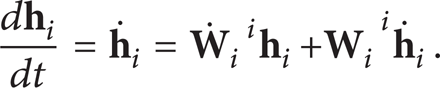
2.4. Velocity of a Point of Link i
Let
Here,
In terms of the fixed inertial coordinates of the base (X
b
Y
b
Z
b
)0, the position 0
Taking the time derivative of the position
To accelerate the computation of the matrices
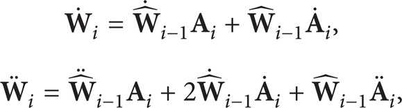
where

Here,

where

3. Dynamics of Flexible Robots
To use Lagrange's equations, we need the kinetic and potential energy of the system.
3.1. The System Kinetic Energy
The system kinetic energy K contains two parts: the links kinetic energy

Assume that the links are slender beams, so the rotary inertia and shear effects can be neglected. Therefore, the present analysis is based on the Euler-Bernoulli beam theory. Also assume that the links can undergo a large overall rigid motion, however the elastic displacements are small. The kinetic energy of the ith link is
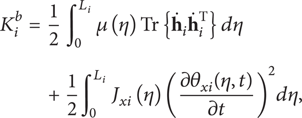
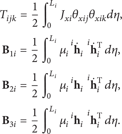
where Tr {·} is the trace operator; μ(η) and J xi are the mass per unit length and the polar moment of inertia per unit length of the link about the neutral axis x, respectively. For slender beams with uniform cross section area along x axis, μ(η) = μ i . The first term in (16) is the kinetic energy of link i accounting for the rigid-body motion and the lateral and longitudinal deformation due to flexibility, whereas the second term is the kinetic energy accounting for the torsional deformation. Note that the torsional angle of link i, θ xi , is expressed as

where δ ij and θ xij are mentioned in (4) and (6), respectively. δ ij is the function of time, whereas θ xij is the function of position η.
Substituting (10) and (17) into (16), expanding it, and then summing over all n links, one finds the links' kinetic energy to be
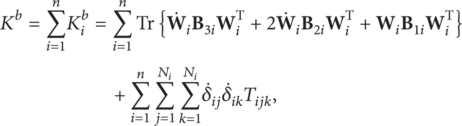
where
With the consideration of
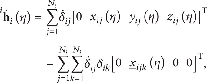
the matrices


where
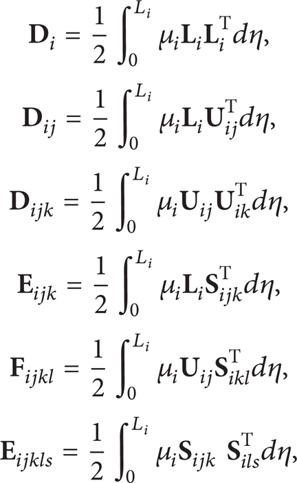
in which

In (21)–(23), the terms with underline remained in high-order approximation coupling model.
It should be noted that the link shape mentioned above is restricted to be the slender beam type. In fact, the link shape can further be extended to the other cases.
Case 1. Link i is the rigid-body with irregular shape. In this case, N
i
= 0,
Case 2. Link i consists of a flexible beam with the concentrated mass m
i
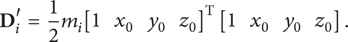
at its proximal end. To account for the contribution of the concentrated mass to the kinetic energy of link i, the extra term
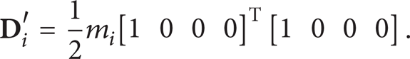
Should the concentrated mass m
i
locate at the position (x0, y0, z0) near the proximal end, the extra matrix
Case 3. Link i consists of a flexible beam with the concentrated mass m
i
at its distal end. Considering the contribution of the concentrated mass to the kinetic energy of link i, the extra terms

For the calculation of the kinetic energy of the joint i, we can lump its mass to link i – 1 in accordance with the assumptions made in [21] for simplicity. Thus, the kinetic energy needs to be included only in the part accounting for spinning kinetic energy of the rotor of joint i as follows:

Considering the relationship in (2). We can obtain the kinetic energy of the joints as follows:

3.2. The System Potential Energy
The potential energy of the flexible manipulators V mainly includes the elastic potential energy of flexible joints V
r
, the elastic potential energy of the flexible links
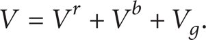
Firstly, the elastic potential energy of joint i is

Secondly, the elastic potential of the flexible links considered here have three parts: one by bending about the transverse y i and z i axes, one by compressing about the longitudinal x i axis, and one by twisting about the longitudinal x i axis. Along an incremental length dη, the elastic potential energy is

Here, θ xi , θ yi , and θ zi are the ith link's rotations of the neutral axis at the point η in the x i , y i , and z i directions, respectively; E i is Young's modulus of material of link i; G i is the shear modulus of material of link i; A xi is the ith link's area of cross section about the x i axis; I yi and I zi are the area moment of inertia of ith link's cross section about the y i and z i axes, respectively; and I xi is the polar area moment of inertia of the ith link's cross section about the neutral axis. Similar to the torsional angle θ xi of (17), θ yi and θ zi can be expressed as

where θ
yik
and θ
zik
are mentioned in (6). By integrating dV
i
b
of (33) over the link, and summing over all n links, one can obtain
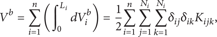
where

Finally, by using the same procedure given by Book [14], the gravity potential of the system is

in which
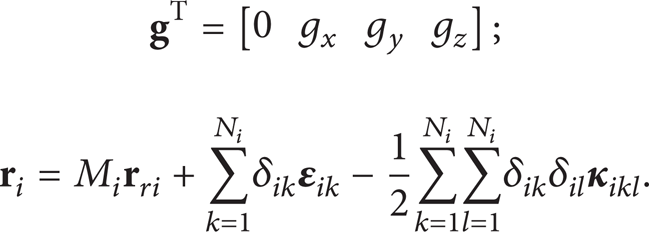
Here, M
i
is the total mass of link i and

Note that
3.3. Dynamic Equations of the System
We use the Lagrange method to derive the dynamics of the system and accord with the method of [14]. Then, the form of Lagrange's equations will be as follows.
For the joint variable q1j, the following simply joint variable equation:

For the joint variable q2j, the following simply joint variable equation:

For the deformation variable δ jf , the following simply deformation variable equation:

Upon the substitution of the system kinetic energy of (15), the system elastic potential energy of (31), and the gravity energy of (37) into (40), (41), and (42), thus becoming as follows.
For the joint variable q1j,

For the joint variables q2j (j = 1, 2, …, n),

For the deformation variables δ jf (j = 1, 2, …, n; f = 1, 2, …, N j ),

Here,
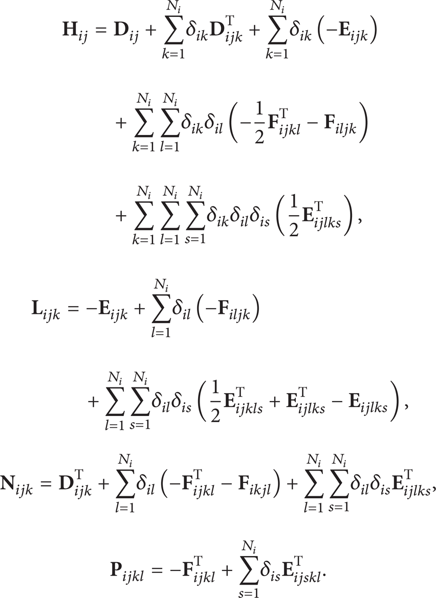
Finally, by complicated derivation and assembling, and using the recursive scheme to reduce the number of calculation, the dynamic equations of the system are obtained in the following formulation:

where the generalized coordinates column

where


(I) In the joint variable equation j (j = 1, 2, …, n), the inertia coefficient J
jh
of the second derivative

where

Here,
(II) In the joint variable equation j (j = 1, 2, …, n), the inertia coefficient J
jhk
of the second derivative
for h = n; j = 1, …, n,

for h = j, …, n – 1; j = 1, …, n – 1,

for h = 1, …, j – 1; j = 2, …, n,

Here,

where
(III) In the joint variable equation j (j = 1, 2, …, n), the inertia coefficients I
jfh
of the second derivative
for j = n; h = 1, …, n,

for j = 1, …, n – 1; h = 1, …, j,

for j = 1, …, n – 1; h = j + 1, …, n – 1,

(IV) In the deformation variable equation j, f, the inertia coefficients I
jfhk
of the second derivative
for j = h = n,

for j = n; h = 1, …, n – 1,

for j = 1, …, n – 1; h = n,

for j = h; h = 1, …, n – 1,

for j = 2, …, n – 1; h = 1, …, j – 1,

for j = 1, …, n – 2; h = j + 1, …, n – 1,

Here,
For the symmetry of the coefficients, we have I jfhk = I hkjf .
(V)

The R rj I is the remains of (43) with the second derivatives removed as follows:

The R Jj I is the remains of (44) with the second derivatives removed as follows:
for j = 1,

for j = 2, …, n,

The R jf I is the remains of (45) with the second derivatives removed as follows.
For j = 1, …, n – 1,

for j = n,

Here,

where the value of

The value of
where
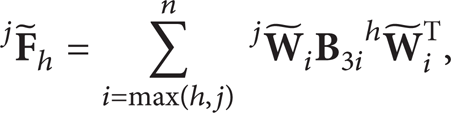
For accelerating the computation of the generalized inertia matrix of the system, the terms

As for
for j = n; h = 1, …, n – 1,
for j = h; h = 1, …, n – 1,

And for j ≠ h ≠ n,

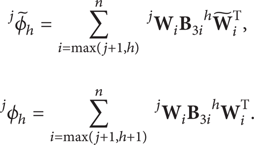
As for

As for
As for j ϕ h , only if N j > 0 and N h > 0, calculate

4. Example of Dynamic Simulation
A general-purpose software package for dynamic simulation of flexible-links and flexible-joints robotic manipulators based on the said algorithm is written in C++. The data structure is pointers and linked lists, so that the data length can be changed based on different initial conditions of the system. The first step is setting up a given interface to input system parameters via reading files. Then, the basic module matrix can be generated automatically. With that, reducing a second order differential equation to a first order linear ordinary differential equation. Eventually, a process based on Adams predictor-corrector method for solving ordinary differential equation calculates till the end time, with an output file per step. It is universal for usage, computationally efficient, and numerically stable.
4.1. Flexible Single-Link Undergoing Low/High Rotational Speed
Ignoring the gravity and the flexible effect of the joint, here, consider the flexible single-link undergoing low/high rotational speed in order to discover the applicability of the high-order geometric nonlinearity coupling model. The properties of the flexible beam are the same as those in [3, 8], and they are given as follows. The length L1 = 8 m, the cross-section area Ax1 = 7.2968 × 10⁻⁵ m2, the area moment of inertia I = 8.2189 × 10⁻⁹ m4, the mass density ρ = 2.7667 × 10³ kg/m3, and the elasticity modulus E1 = 6.8952 × 10¹⁰ N/m2. For the flexible cantilever beam without large overall motion, the fundamental frequency is 0.464 Hz. The large rotating motion law of the system adopted

where T = 15 s, and ω0 is chosen here to be 0.6, 2, 3, 8, and 10 rad/s, respectively, in the following numerical simulations. The tip deformations of link u y are shown from Figures 3, 4, and 5.

ω0 < 3 rad/s.

ω0 = 3 rad/s.
ω0 > 3 rad/s.
It can be observed that, undergoing a low rotating speed (0.6 rad/s or 2 rad/s), there is an obvious difference between zero-order and high-order coupling model, and the difference becomes larger and larger with the increasing of the rotating speed. When the high-order coupling model is at the rotating speed 3 rad/s (≈0.477 Hz), closing to the fundamental frequency (0.464 Hz), the vibrating amplitude of the link tip is aroused much higher, but it is convergent. Whereas, the results form zero-order coupling model turn to be divergente. When reaching a high rotating speed, 8 rad/s (≈1.272 Hz) or 10 rad/s (≈1.59 Hz), the zero-order coupling model will fail to get the convergent results. These phenomena are coincided with the numerical result in [2, 11].
4.2. Spatial Flexible-Link and Flexible-Joint Robotic Arm
In order to validate the algorithm and package presented in this paper, the dynamic simulation of Canadarm2 (the Space Station remote manipulator system serving on the international space station) is given as an example.
As shown in Figure 6, Canadarm2 consists of four parts: shoulder, upper arm boom, lower arm boom, and wrist, in which the shoulder and the wrist both have 3 rotational degrees of freedom (DOF), and the elbow connecting the upper arm and the lower arm has 1 rotational DOF. Hence, the total system can be regarded as a 7-DOF manipulator with seven links and seven revolute joints. The links making up the shoulder and the wrist are short and thick in shape; therefore, they can be regarded as rigid links, whereas the upper and lower arms are assumed to be flexible due to their slender beam type. Therefore, Canadarm2 system is simplified to contain two flexible links and three rigid links which are connected through flexible joints, as shown in Figure 7. In this example, there is a distance d = 0.475 m between the 2nd link and 1st link along the Z-axis, which consequently arouse the rotation of the flexible links. And the longitudinal stretching (along X-axis), transversal bending (along Y-axis and Z-axis), and torsion (around X-axis) are considered here. Correspondingly, a total of 12 eigenfunctions (the first three preorientation of deformation) of a clamped-free beam are utilized to represent the mode shapes of each link deformation. The links parameters are shown in Table 1. The material of the links is aluminum, cross-section parameter E i I yi = E i I zi = 3.8 × 10⁶ Nm2, E i A i = 2.84 × 10⁷ N, G i = 0.27 × 10⁵ MPa, and J xi = 15.41 kg × m2. Initial joint angle is q11 = 0.4π rad, q21 = 0.4π rad, q12 = – 0.4π rad, and q22 = – 0.4π rad, respectively. Initial joint angle velocity is zero.
The parameters of space robot system.


The space robot arm Canadarm2.
A spatial flexible robot arms.
4.2.1. Dropping Motion in the Gravity Field
Figure 8 describes the motion of the high-order coupling flexible five-links system dropping in the gravity field.
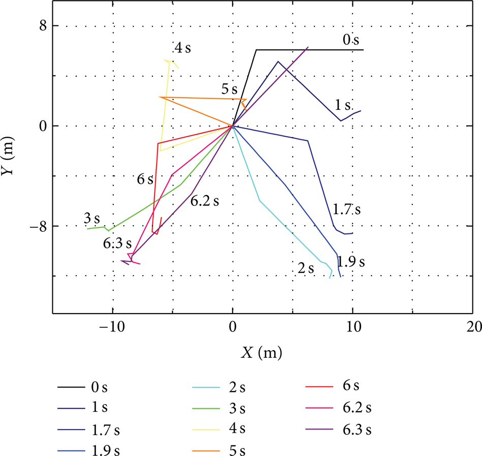
The flexible robot arms motion.
4.2.2. Effects of Joint Flexibility on the System
Figure 9 shows the torsional angle of the 1st joint ∊1 in the high-order coupling model with different mass J ri n i 2, 5, 10, or 15, respectively. Figures 10, 11, 12, and 13 show the X, Y, and Z deformation u x , v y , w z , and torsional angle θ x of 1st link tip with different joint mass. The larger joint's mass is, the larger joint angles of motion the system has. The same phenomena can be seen form Figures 10 to 13.
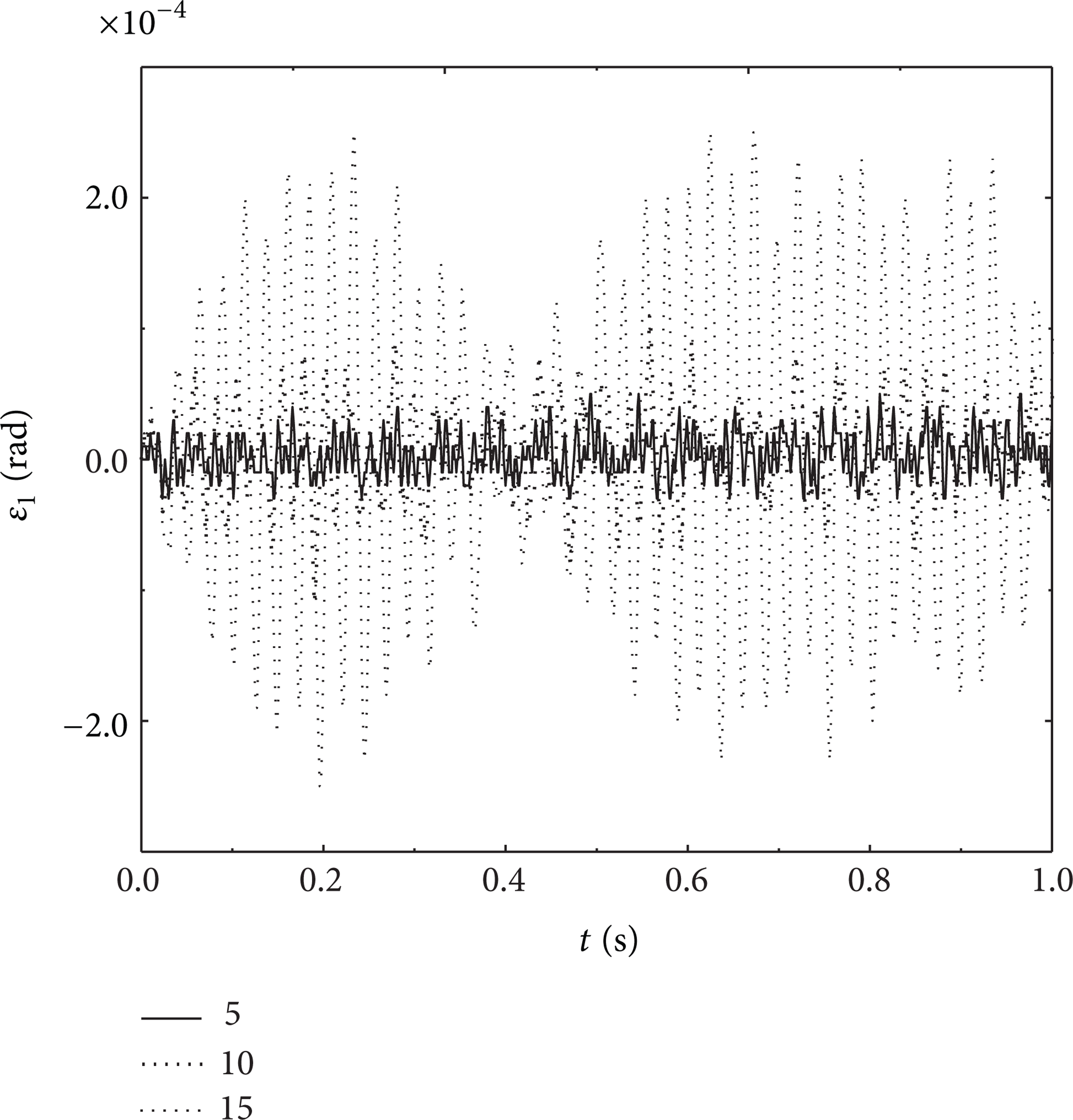
The torsional angle of 1st joint, ∊1.
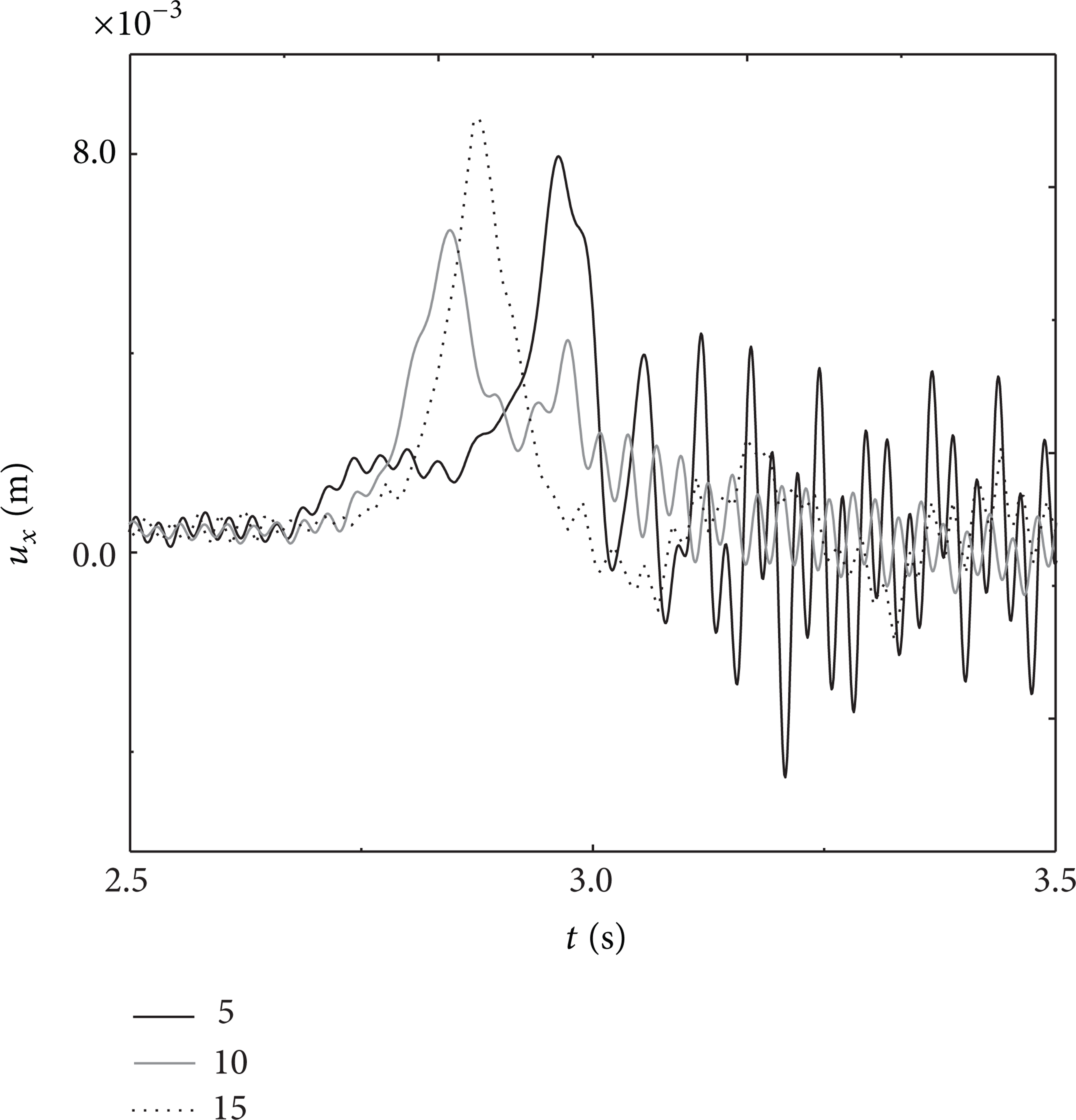
u x of 1st link tip.

v y of 1st link tip.

w z of 1st link tip.

θ x of 1st link tip.
The real rotational angle q2i of five joint in the high-order coupling model is shown in Figures 14, 15, 16, 17, and 18 with different stiffness. The joint stiffness Kt i is chosen here to be 0.60, 1.33, 2.66, and 5.00 × 10⁶ N/mm, respectively.
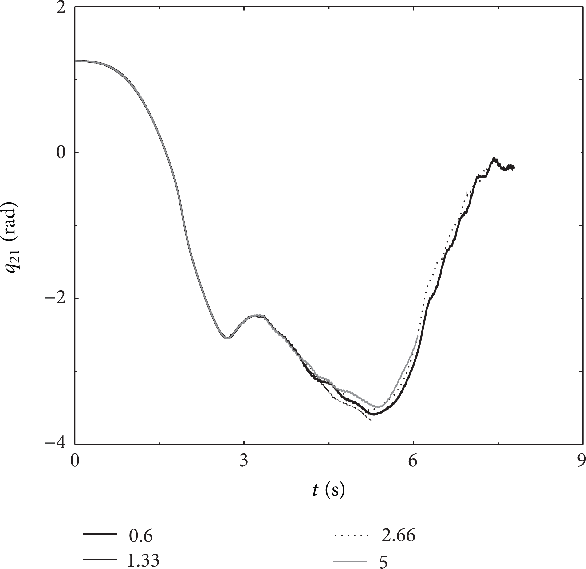
The 1st joint, q21.

The 2nd joint, q22.
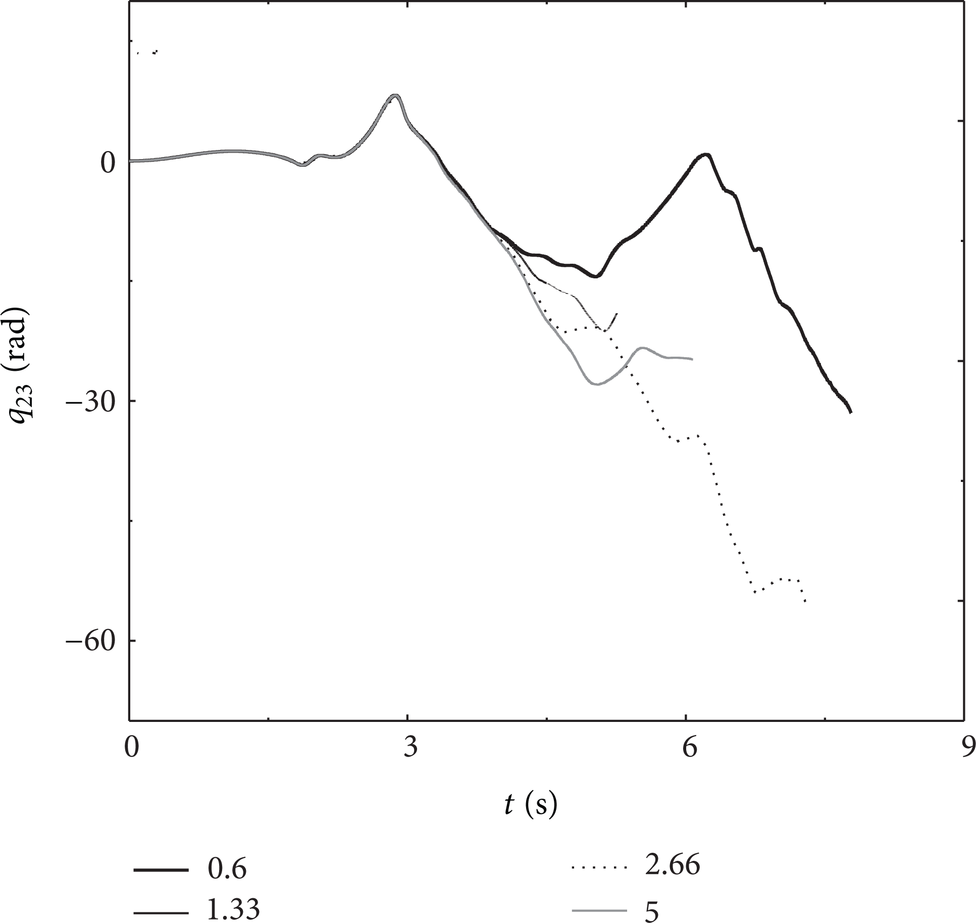
The 3rd joint, q23.
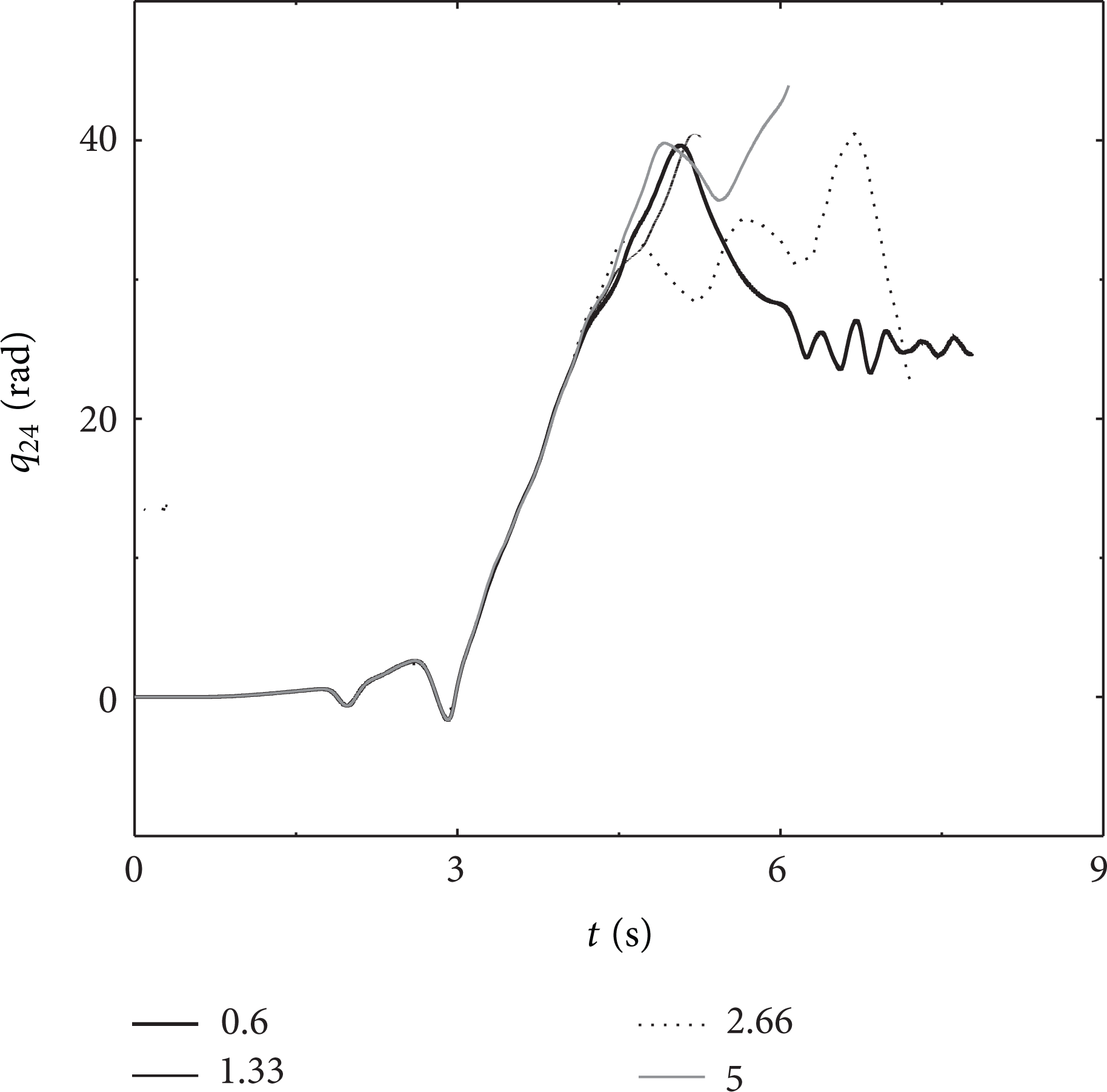
The 4th joint, q24.

The 5th joint, q25.
5. Conclusions
This paper aims at building a comprehensive model of spatial manipulator arms consisting of n flexible links and n flexible joints. The deformations of stretching, bending, and torsion of the links are all considered. And the flexibility and the mass of the joints are also included. In the modeling, the so-called dynamic stiffening effects are considered via the adoption of nonlinear deformation description. Based on the presented method, a general-purpose software package of multilink manipulator arms is developed. The results demonstrate that dynamic stiffening effects cannot be neglected. The coupling effects of flexible links and flexible joints on dynamic characteristics are significant to the system's accurate dynamic response predictions, performance evaluation, and implementation of procedure control.
Footnotes
Acknowledgments
This work is supported by the National Natural Science Foundations of China (11272155, 11132007, and 10772085), 333 Project of Jiangsu Province (BRA2011172), and the Fundamental Research Funds for Central Universities (30920130112009).