
Abstract
The properties of interpolation of nodal data, ease of imposing essential boundary conditions, and the computational efficiency are some of the most important advantages of natural element method based on the non-Sibsonian interpolation over other meshless methods based on the moving least squares approximants. Accurate imposition of essential boundary conditions is accomplished directly by constructing vector of the displacement field by using non-Sibsonian interpolation method, which is based on the Voronoi diagram and its dual Delaunay tessellation. The discrete control equations of natural element method are developed by utilizing the variational principle of elastic theory and combining the natural element method with the theory of the linear elastic fracture mechanics. Without the connectivity information of elements, the burdensome remeshing, which is used in finite element method, is avoided in the present natural element method. The analysis of crack propagation is simplified dramatically. The numerical examples reveal the advantages and effectiveness of the present method.
1. Introduction
The simulation of crack propagation by using various numerical methods is an important field in the areas of mechanics and engineering to determine fracture response and reliability of cracked structures. Although FEM has numerous advantages, the method has serious limitations in solving the problem of crack propagation characterized by a continuous change in geometry of the domain under analysis. A large number of remeshings are required in the finite element model to represent arbitrary and complex paths. The underlying structures of FEM and similar methods, which rely on a mesh, are quite cumbersome in treating cracks that are not coincident with the original mesh geometry. Consequently, the only viable option for dealing with moving cracks using the FEM is to remesh during each discrete step of model evolution so that mesh lines remain coincident with cracks throughout the analysis. This creates numerical difficulties, often leading to degradation of solution accuracy, complexity in computer programming, and a computationally intensive environment.
A class of meshless methods, in which a structured mesh is not used and only a scattered set of nodal points is required in the domain of interest, is proposed to overcome the difficulties of the methods requiring remeshings. Since the domain of interest is discretized completely by a set of nodes, the meshless method presents significant implications for the analysis of the problem of the fracture mechanics [1–5]. With the development of the meshless method, the natural element method (NEM) [6–10], which is based on the Voronoi diagram and Delaunay triangulation, is built upon the notion of the natural neighbor interpolation. As its shape functions satisfy interpolating properties, the natural element method is similar to the finite element method and can exactly interpolate piece. The natural element method has advantages of both finite element method and meshless method.
In the present paper, accurate imposition of displacement boundary conditions is accomplished directly by constructing vector of the displacement field by using the non-Sibsonian interpolation method. The discrete governing equations of natural element method are developed by utilizing the variational principle of elastic materials. By combining the natural element method with the theory of linear elastic fracture mechanics, the natural element method is used to calculate the stress intensity factors by using the J-integral method and the contour integral method. The crack propagation of edge-oblique-cracked rectangular plate is also simulated by employing the theory of the maximum circumferential stress criterion and the increment of crack length during each step of crack propagation.
2. Analysis Method
2.1. Basic Principle of Natural Element Method
The non-Sibson interpolation is constructed on the basis of the underlying Voronoi tessellation, which is unique for a given set of distinct points (nodes) in the plane. The Delaunay triangles which are the dual of the Voronoi diagram are used in the numerical computation of NEM. Figure 1 shows the Voronoi diagram and the Delaunay triangulation. Figure 2 shows the non-Sibson interpolation of the arbitrary point
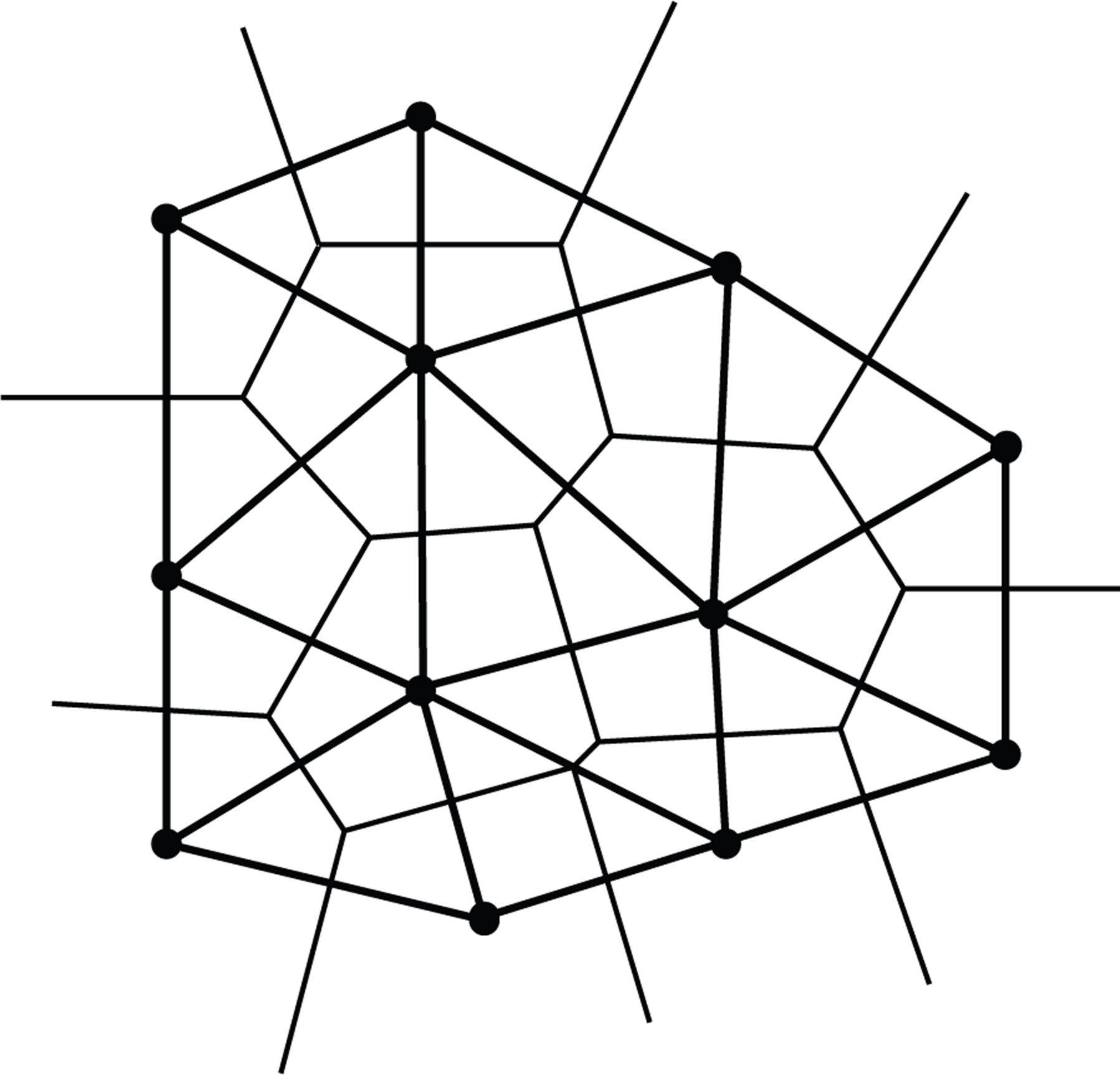
Voronoi's diagram and its Delaunay tessellation.

Non-Sibson interpolation.
The displacement of an arbitrary point

where

where n is the number of the natural neighbor node of the arbitrary point
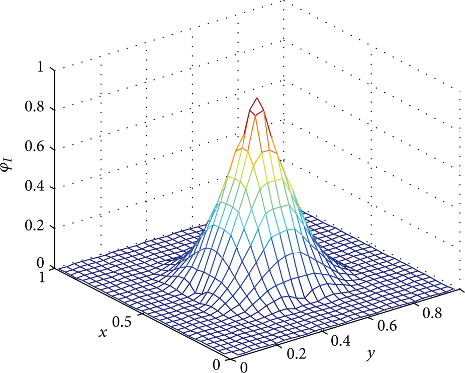
Shape function of the non-Sibson interpolation.
The derivatives of φ
I
(
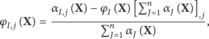
where φI, j(
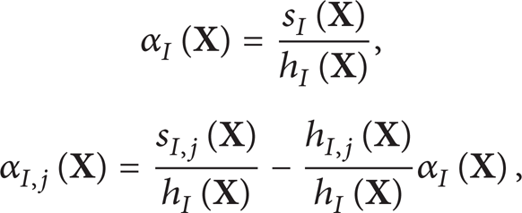
where h
I
(
Constructing the vector of displacement with the expression (1), the energy functional Π of the problem of the elastic mechanics is as follows:

where
The discrete control equations of the natural element method can be developed by substituting expression (1) into expression (6), letting the variation of Π be zero, namely, δΠ = 0, and using the arbitrary of the variation:

where


where I, J = 1, 2, …, N P .
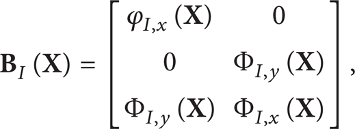
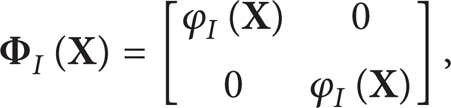
In the two-dimensional problem, the expressions of
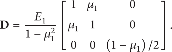
For the plane stress problem, E1 = E, μ1 = μ. For the plane strain problem, E1 = E/(1 – μ2), μ1 = μ/(1 – μ), and E and μare the modulus of elasticity and the Poisson ratio, respectively.
2.2. Simulation of Crack Propagation
(1) Criterion of Crack Propagation. The results of experiment show that the cracking and the propagation of the mixed mode crack do not along the direction of the old crack surface generally. In order to simulate the propagation of the I-II mixed-mode cracks of the linear elastic material, besides the determination of the crack propagation criterion, the crack-path direction, which is called the cracking angle, should also be determined. There are several criteria available to predict the direction of crack trajectory. They are the maximum tension stress theory [11], the maximum energy release rate theory [12], and the minimum strain energy density theory [13]. The maximum tension stress theory was used to simulate the crack growth in the present study.
According to the maximum circumferential stress criterion [11], the initial crack propagates along the direction of the maximum circumferential stress. The relationship of the direction of crack propagation θ with the stress intensity factor KI and KII is as follows:

where the cracking angle θ is the angle between the direction of the old crack and the direction of the crack propagation.
The fracture criterion of the I-II mixed-mode cracks is as follows by adopting the maximum circumferential stress criterion:

where Kθ and KIc are the equivalent stress intensity factor and the fracture toughness, respectively.
(2) The Selection of the Crack-Length Increment and the Update of the Crack Geometry. Since the actual process of the crack propagation is a nonlinear dynamic process, the continuous process was separated into the incremental form which includes a set of linear incremental steps. Figure 4 shows the configuration after one incremental step of crack propagation. The crack propagation of each increment is considered as a steady-state process, in which the change of the stress field is ignored and the crack propagated along the line segment da. The choice of the increment of crack length da has the direct influence on the simulation results. If da is too big, the idea of replacing the nonlinearity with the linearity in a small range will be deviated. The result of simulation will deviate from the reality because the error increased largely. Though the computing precision will increase when da is very small, the computing efficiency will slack down. According to the calculation practice of the present paper, the increment of crack length during each step of crack propagation is a constant in each crack growth, which is from 1/20 to 1/10 of the initial crack length. After each increment, the meshless node in the old crack-tip is split into two nodes locating on the opposite sides of the crack. The distance between the new crack-tip and the old crack-tip is da. Therefore, the geometry of the crack should be updated after each incremental step of the crack propagation.
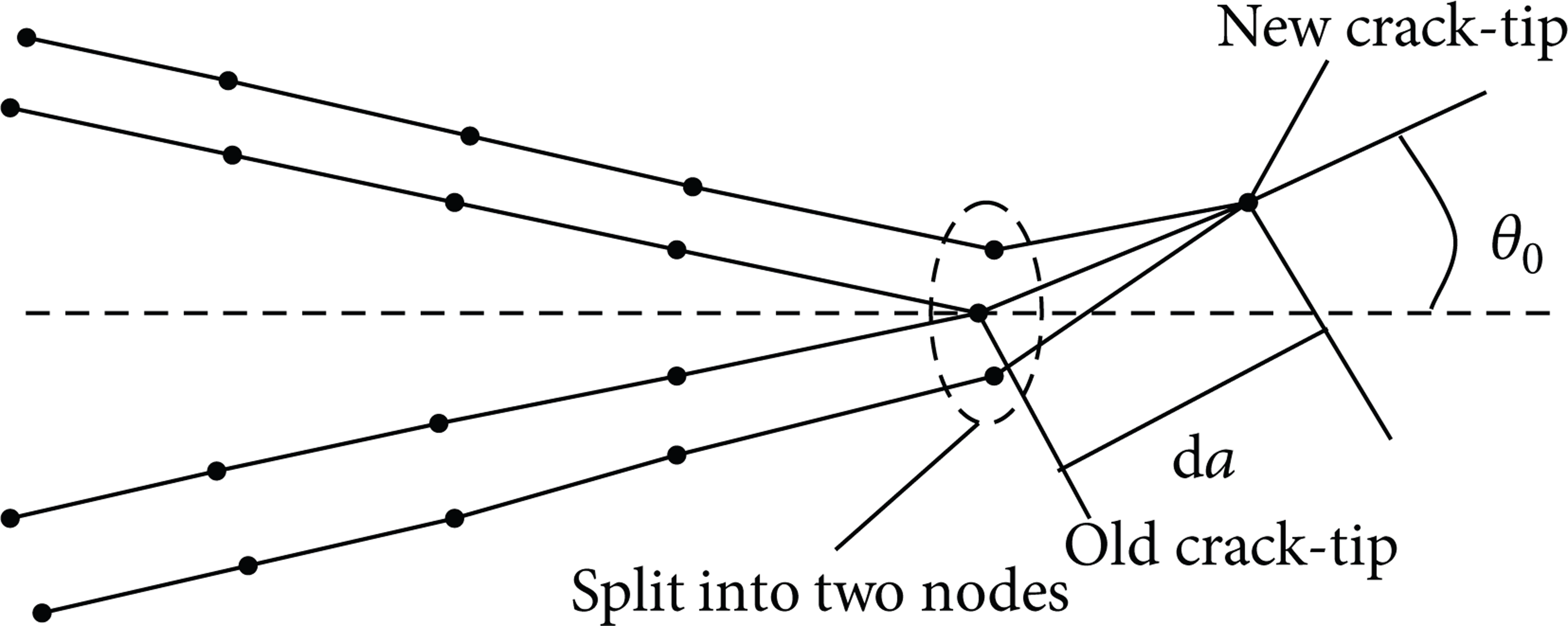
Configuration after one incremental step of crack propagation.
In Figure 4, let the coordinates of the initial crack-tip be (x0, y0). The angle between the initial crack and the positive x-axis is β0. The initial cracking angle is θ0. Let the coordinate of the crack-tip after the ith increment be (x i , y i ). The angle between the ith crack increment and the positive x-axis is β i = βi – 1 + θi – 1, where θ i is the angle of the ith crack propagation, which is the angle rotated from the direction of the (i – 1) th crack propagation to the direction of the ith crack propagation in counterclockwise direction. The coordinate (x i , y i ) can be calculated as follows:


The old crack-tip is split into two nodes locating on the opposite sides of the crack. In the present study, the distance between the two new nodes is set to 0.0002 units, which is the width of the initial crack in the following present numerical example of the crack propagation of the edge-oblique-cracked plate. The coordinates of the nodes can be calculated by the following vectors including the x-coordinates and the y-coordinates of the 3 points, respectively:

The three points of the ith crack increment include the ith crack tip and the two nodes locating on the opposite sides of the crack. The coordinates of the two nodes locating on the opposite sides of the crack are calculated by using the transformation of coordinates.
3. Numerical Examples
According to the above numerical method, the corresponding MATLAB program has been made to study the application of the natural element method on the linear elastic fracture mechanics.
3.1. Stress Intensity Factor of Rectangular Plate with a Mode I Central Crack
A rectangular plate with a central crack is considered. Due to symmetry, only half of the plate is analyzed. The mechanical model of the cracked plate under pure tension is as shown in Figure 5, that has width, w = 1 m, height, h = 2 m, and crack length, a = 0.4 m. The far-field tensile stress is σ = 1.0 Pa. The Young modulus and the Poisson ratio are E = 2.07 × 10¹¹ Pa and ν = 0.3, respectively.
Mechanical model of the rectangular plate with a mode I central crack.
A discrete model consisting of 263 meshless nodes is shown in Figure 6. The domain Q1Q2Q3Q4 of size c × c required for calculating the J-integral is defined in Figure 6.

Discrete model of the rectangular plate with a mode I central crack.
Table 1 shows the values of stress intensity factor KI under various J-integral contours, where the relationship between the stress intensity factor KI0 and the correction coefficient FI is
Computational results of stress intensity factors KI under different integral contours.

3.2. Crack Propagation of the Edge-Oblique-Cracked Plate
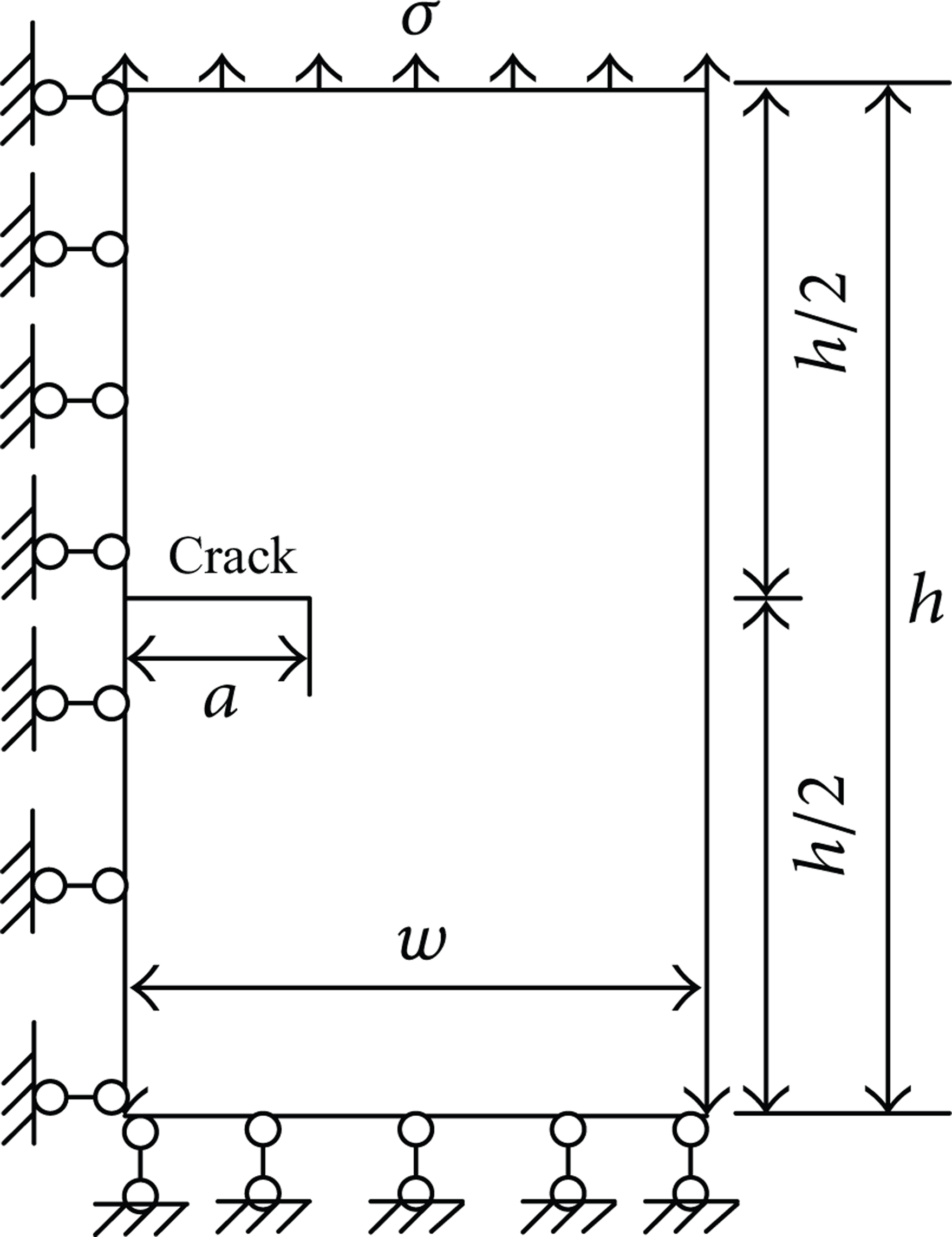
Figure 7 shows the mechanical model of an edge-oblique-cracked rectangular plate, which has width, b = 1 m, height, h = 2.5b, and initial crack length, a = 0.5 m at α = 45°. The discrete model is shown in Figure 8. In calculation, the contour integral method [15] and the Gauss integration based on the Delaunay triangles are used. The stress of far-field tensile, σ = 1 Pa. The Young modulus and the Poisson ratio are E = 2.07 × 10¹¹ Pa and ν = 0.25, respectively.

Mechanical model of the rectangular plate with unilateral oblique crack.
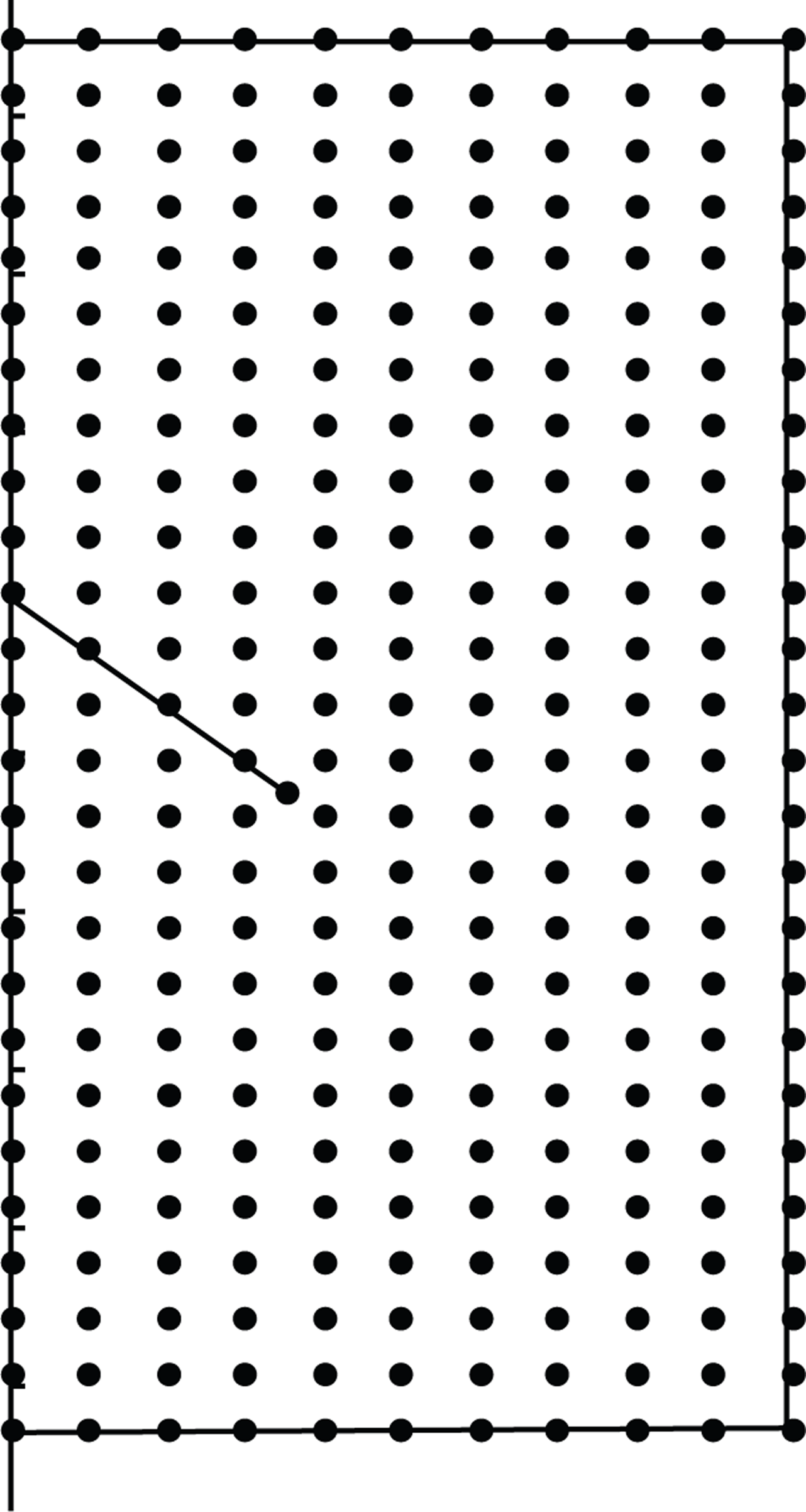
Discrete model of the rectangular plate with a unilateral oblique crack.
Table 2 shows the values of stress intensity factors KI and KII by using the present method and the element-free Galerkin method [16] (EFGM), respectively. It can be seen that the present method has better accuracy when it is used to calculate the stress intensity factor of the oblique crack.
Computational results of stress intensity factors of unilateral shear crack.

Figure 9 shows the predicted crack trajectories of the rectangular plate with a unilateral oblique crack by the proposed natural element method. In the calculation, the far-field tensile stress, σ = 2 × 10⁶ Pa. The fracture toughness,
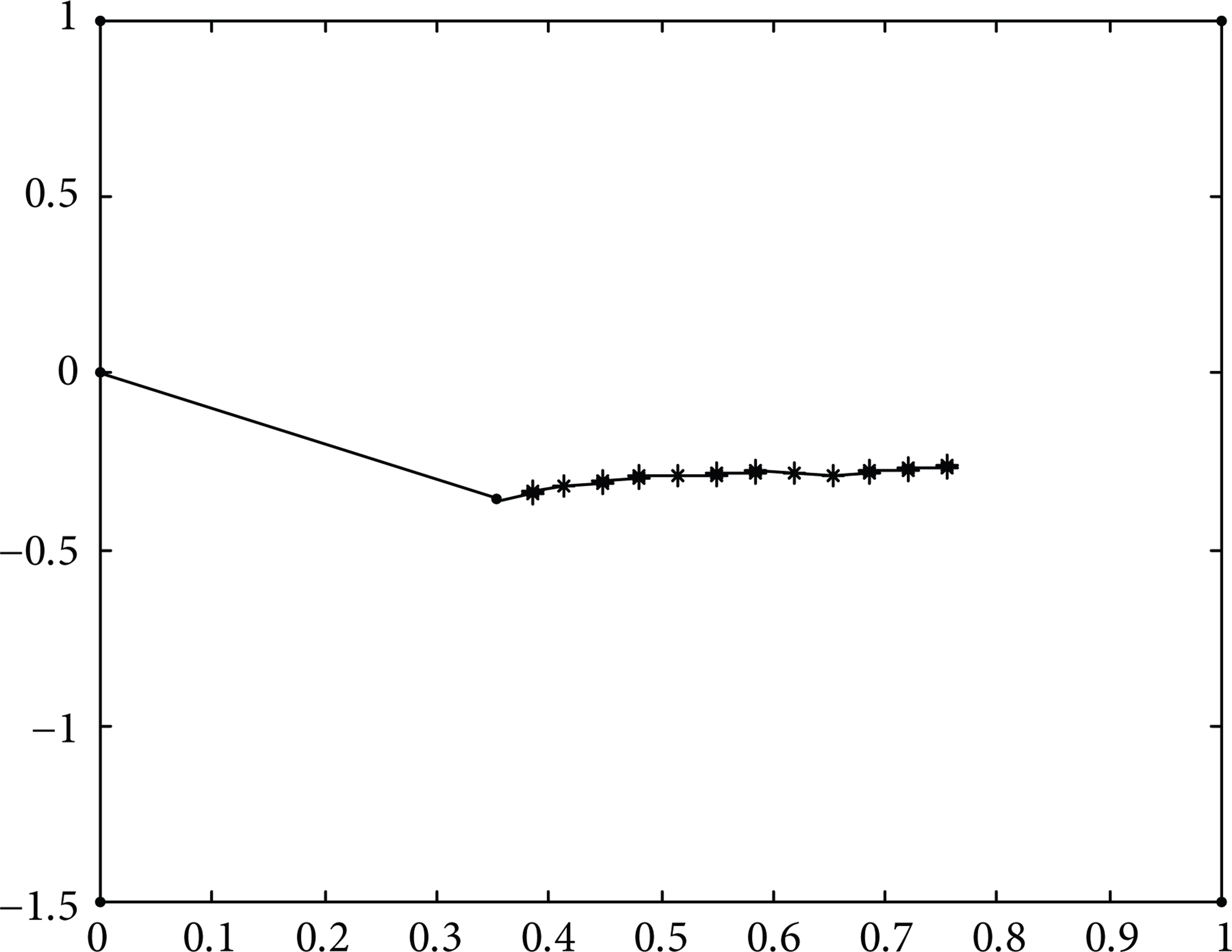
Crack path of the rectangular plate with a unilateral oblique crack after 12 steps of crack propagation.
4. Conclusions
Accurate imposition of essential boundary conditions was accomplished directly in the present paper by constructing vector of the displacement field by using non-Sibsonian interpolation. The stress intensity factor was calculated by using the J-integral method and the contour integral method. The natural element method was used to simulate the crack propagation of an edge-oblique-cracked rectangular plate by using the maximum circumferential stress criterion and the increment of crack length during each step of crack propagation. The natural element method based on the non-Sibsonian interpolation is not only convenient on the accurate imposition of the essential boundary conditions, but also it can simulate the crack propagation of the unilateral oblique crack. Since no element connectivity data are needed, the burdensome remeshing required by FEM is avoided. A growing crack can be modeled by simply extending the free surfaces, which correspond to the crack. Therefore, the complex analysis of crack-propagation can be significantly reduced by using the natural element method and sidestepping the requirements of remeshing.
Footnotes
Acknowledgments
The present investigation has been sponsored by the National Science Foundation of China (no. 51279095), the Science Foundation of Shandong Province of China (ZR2010EM032), Independent Innovation Foundation of Shandong University (IIFSDU2012ZD033), and the Special Funding of Postdoctoral Innovation Projects of Shandong Province (201102011).