Time Synchronization in Wireless Sensor Networks Using Max and Average Consensus Protocol

Abstract

This paper proposes a novel distributed time synchronization scheme for wireless sensor networks, which uses max consensus to compensate for clock drift and average consensus to compensate for clock offset. The main idea is to achieve a global synchronization just using local information. The proposed protocol has the advantage of being totally distributed, asynchronous, and robust to packet drop and sensor node failure. Finally, the protocol has been implemented in MATLAB. Through several simulations, we can see that this protocol can reduce clock error to ±10 ticks, adapt to dynamic topology, and be suitable to large-scale applications.

1. Introduction

As in all distributed systems, time synchronization is very important in wireless sensor networks (WSNs) since the design of many protocols and implementation of applications require precise time, for example, forming an energy-efficient radio schedule, conducting in-network processing (data fusion, data suppression, data reduction, etc.), distributing an acoustic beamforming array, performing acoustic ranging (i.e., measuring the time of flight of sound), logging causal events during system debugging, and querying a distributed database.

Time synchronization is a research area with a very long history. Various mechanisms and algorithms have been proposed and extensively used over the past few decades. However, several unique characteristics of WSNs often preclude the use of the existing synchronization techniques in this domain. First, since the amount of energy available to battery-powered sensors is quite limited, time synchronization must be implemented in an energy-efficient way. Second, some messages need to be exchanged for achieving synchronization while limited bandwidth of wireless communication discourages frequent message exchanges among sensor nodes. Third, the small size of a sensor node imposes restrictions on computational power and storage space. Therefore, traditional synchronization schemes such as network time protocol (NTP) and global positioning system (GPS) are not suitable for WSNs because of complexity and energy issues, cost efficiency, limited size, and so on.

In the context of WSNs, time synchronization refers to the problem of synchronizing clocks across a set of sensor nodes that are connected to one another over a single-hop or multihop wireless networks. To achieve time synchronization in wireless sensor networks, we have to face the following four challenges.

1.1. Nondeterministic Delays

There are many sources of message delivery delays. Kopetz and Ochsenreiter [1] describe the components of message latency, which they call the Reading Error, as being comprised of 4 distinct components plus the local granularity of the nodes clocks. Their work was later expanded by [2] to include transmission and reception time. The most nondeterministic delay is called Access Time, which is incurred in the MAC layer waiting for access to the transmit channel, its orders of magnitude is larger than the synchronization precision required by the network.

1.2. Clock Drift

Manufacturers of crystal oscillators specify a tolerance value in parts per million (PPM) relative the nominal frequency at 25°C, which determines the maximum amount that the skew rate will deviate from 1. For the nodes used in WSNs, the tolerance value is typically in the order of 5 to 20 PPM. If no drift compensation applied, two synchronized nodes will be out of step soon.

1.3. Robustness

Since sensor networks are often left unattended for long periods of time in possibly hostile environments, synchronization schemes should be robust against link and node failures. Mobile nodes can also disrupt routing schemes, and network partitioning may occur.

1.4. Convergence Speed

Nodes in wireless sensor networks always distribute in large scales, one node may get in touch with another by many hops. This increases the difficulty in reducing the convergence speed in time synchronization algorithm design.

Up to now, many protocols have been designed to address this problem. These protocols all have some basic features in common: a simple connectionless messaging protocol, exchange of clock information among nodes, mitigating the effect of nondeterministic factors in message delivery, and processing utilizing different schemes and algorithms, respectively. They can be classified into two types: centralized synchronization and distributed synchronization.

Centralized synchronization protocol, such as RBS [4], TPSN [2], and FTSP [3], usually has fast convergence speed and little synchronization error. This kind of protocol needs a physical node acting as the whole network's reference clock, so it has to divide the nodes into different roles, for example, client node and beacon node in RBS. If the node with the special role, such as beacon node in RBS, is out of work, the protocol will suffer from big damage. To deal with the WSNs' dynamic topology, centralized synchronization protocol is often designed with complexity logic. Another disadvantage of centralized synchronization protocol is that synchronization error grows with the increase of network hops.

Distributed synchronization protocol, such as TDP [5]/GCS [6]/RFA [7]/ATS [8]/CCS [9], can use local information to achieve the whole network synchronization. This kind of protocol can easily adapt to WSNs' dynamic topology property with lite computation. Currently, the disadvantage of distributed synchronization protocol is that the convergence speed may be a bit slow, relating to the network topology.

This paper describes a new distributed protocol for time synchronization in wireless sensor networks called time synchronization using max and average consensus protocol (TSMA). We adapt a number of techniques to take up the challenges time synchronization has in WSNs. To eliminate the nondeterministic delays, we make use of MAC layer timestamp technique. To compensate for the clock drift, we adapt max consensus protocol, and we use average consensus protocol to compensate for the clock offset. This protocol has the advantages of being computationally light, scalable, asynchronous, robust to node and link failure, and it does not require a master or controlling node.

The rest of the paper is organized as follows. Section 2 summarizes the related work. Section 3 introduces some mathematical tools and definitions that will be instrumental for the proof of convergence of the proposed TSMA algorithm. Section 4 introduces a model for the clock dynamics and formally defines the synchronization objectives, while Section 5 presents the TSMA algorithm in details. This is followed by MATLAB simulations in Section 6. Finally, Section 7 briefly summarizes the results obtained and proposes potential research directions.

2. Related Work

Typical time synchronization algorithms in WSNs include timing-sync protocol for sensor networks (TPSNs) [2], reference broadcast synchronization (RBS) [4], flooding time synchronization protocol (FTSP) [3], time diffusion protocol (TDP) [5], global clock synchronization (GCS) [6], Reachback Firefly algorithm (RFA) [7], average time synchronization (ATS) [8], and consensus clock synchronization (CCS) [9]. RBS, TPSN, and FTSP are centralized synchronization protocols, while TDP, GCS, RFA, ATS, and CCS are distributed synchronization protocols.

TPSN [2] is designed as a flexible extension of NTP [10] for use in wireless sensor networks, which consists of two phases: a level discovery phase and a synchronization phase. The level discovery phase organizes the whole network into a hierarchical tree topology with the master node at its root, then perform the pair wise synchronization along the branches of the hierarchical structure using the classical sender-receiver synchronization handshake exchange in the synchronization phase. TPSN is a centralized synchronization protocol, utilizes MAC layer timestamping to reduce message delivery nondeterminism and improve synchronization accuracy, its convergence speed increases linearly with the max network hops. This approach suffers from two limitations. The first limitation arises because if the root node or parent node dies, then a new root election or parent-discovery procedure needs to be initiated, thus adding substantial overhead to the code and long periods of network desynchronization. The second limitation is due to the fact that geographically closed nodes might be far in terms of the tree distance, which is directly related to increase the clocks error locally.

RBS [4] aims to provide synchronization amongst a set of client nodes located within the single-hop broadcast range of a beacon node. Compared to the traditional protocols working on an LAN, its main contribution is to directly remove two of the largest sources of nondeterminism involved in message transmission, transmission time, and access time, by exploiting the concept of a time critical path, which is the path of a message that contributes to nondeterministic synchronization errors. This centralized protocol uses least squares linear regression to compensate for the clock drift, its convergence speed also increases linearly with the max network hops. Using the beacon node makes this protocol vulnerable to node failure and node mobility.

FTSP [3] is an ad-hoc, multihop time synchronization protocol for WSNs. It achieves high accuracy by utilizing timestamping of radio messages in low layers of radio stack, completely eliminating access time to the radio channel required in CSMA MAC protocols. Further accuracy is achieved by compensating for clock skews of participating nodes via linear regression. Several mechanisms are used to provide robustness against node and link failures, most notably periodic flooding of synchronization messages throughout the whole network, but this approach still do not completely solve the limitations aforementioned in TPSN.

Nodes employing TDP [5] periodically self-determine to become master/diffusion leader nodes using an election/re-election procedure. Master nodes then engage neighboring nodes in a peer evaluation procedure to isolate problem nodes. Timing information messages are broadcasted from master nodes and then rebroadcasted by the diffused leader nodes for a fixed number of hops, forming a radial tree structure. This approach is fully distributed, but it does not compensate for the clock drift. To the application needing small tolerance time, this algorithm has to increase the synchronization frequency, which greatly decreases the node's battery life.

In GCS [6], nodes take turns to broadcast a synchronization request to their neighbors who each respond with a message containing their local time. The receiving node (at the center of this exchange) averages the received time-stamps and broadcasts this value back to its neighbors which adopt this value as their new time. This is repeated by each node in the network until network wide synchronization is achieved. This approach is fully distributed, but it does not compensate for the clock drift. To get higher time accuracy, it has to decrease the time synchronization period.

RFA [7] is inspired by firefly synchronization mechanism. In this algorithm, every node periodically broadcasts a synchronization message, and anytime they hear a message they advance, of a small quantity, the phase of their internal clock that schedules the periodic message broadcasting. Eventually all nodes will advance their phase till they are all synchronized, that is, they fire a message at the same time. This approach, however, does not compensate for clock drift, therefore the firing period needs to be rather small.

ATS [8] uses a cascade of two consensus algorithms to tune compensation parameters and converge nodes to a steady state virtual clock. In the first stage, nodes broadcast local timestamps in order to estimate the clock skew rates relative to each other. Nodes then broadcast their current estimate of the virtual clock skew rate and receiving nodes combine this with their relative skew estimates to adjust their own virtual clock estimate. The same principle is then applied to remove the offset errors. This is a fully distributed protocol; its convergence speed is a bit slow, related to the network topology.

CCS [9] utilizes average consensus algorithm to compensate the clock offset. By the accumulated offset error that they remove during each round of offset compensation nodes can observe how much their own clocks drift away from the consensus time, then they use this information to compensate the clock drift, which can be seen as an enhancement of ATS. This approach is also fully distributed and has the disadvantage of slow convergence speed.

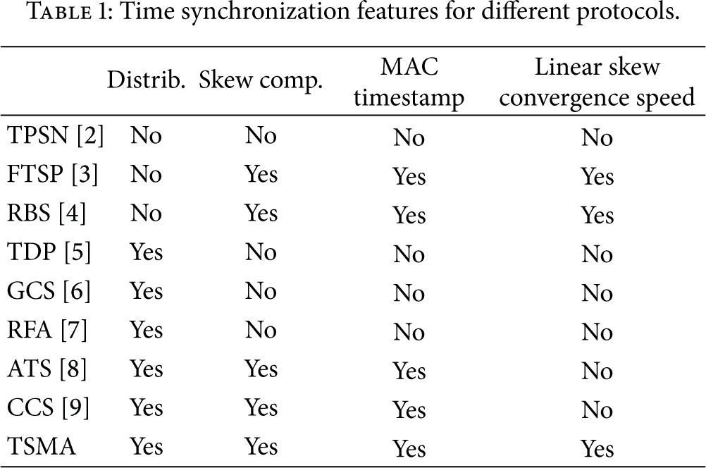
The TSMA protocol proposed in this paper is similar to ATS and CCS. It is fully distributed, that is, it does not require any special root, including skew compensation, and exploits MAC-layer timestamping for higher accuracy. Unlike ATS and CCS, the proposed protocol uses max consensus method to compensate the clock drift, which has faster skew convergence speed as the centralized protocol, that is, it increases linearly with the max network hops. The features of all the protocols mentioned in this section are summarized in Table 1.

Table 1

Time synchronization features for different protocols.

	Distrib.	Skew comp.	MAC timestamp	Linear skew convergence speed
TPSN [2]	No	No	No	No
FTSP [3]	No	Yes	Yes	Yes
RBS [4]	No	Yes	Yes	Yes
TDP [5]	Yes	No	No	No
GCS [6]	Yes	No	No	No
RFA [7]	Yes	No	No	No
ATS [8]	Yes	Yes	Yes	No
CCS [9]	Yes	Yes	Yes	No
TSMA	Yes	Yes	Yes	Yes

3. Mathematical Preliminaries

We assume that links in WSNs are symmetric, so the network can be modeled as an undirected graph $G=(V,E)$ , where $V=\{v_i\mid i=\mathrm{1,2},\dots ,n\}$ represents the nodes in the WSNs, and the edge set E represents the available communication links, that is, $(v_i,v_j)\in E$ if node j sends information to node i. We refer to $v_i$ and $v_j$ as the tail and head of the edge $(v_i,v_j)$ , respectively. The orientation of the graph is a choice of heads and tails for each undirected edge. The set of edges of a fix orientation of the graph is denoted by $E_{\mathrm{0}}$ . Thus, $E_{\mathrm{0}}$ contains one and only one of the two edges $(v_i,v_j),\mathrm{\hspace{0.17em}\hspace{0.17em}}(v_j,v_i)\in E$ . We use m to present edge number and n the vertex number, for example, $n=|V|,\mathrm{\hspace{0.17em}\hspace{0.17em}}m=|E_{\mathrm{0}}|$ . The set of neighbors of node is denoted by $N_i=\{v_j\mid e_{i,j}\in E\}$ . The degree of node $v_i$ is the number of its neighbors $|N_i|$ and is denoted by $\mathrm{deg}(v_i)$ . The degree matrix is an $n\times n$ matrix defined as $\mathrm{\Delta }=\mathrm{\Delta }(G)=\{{\mathrm{\Delta }}_{e_{i,j}}\}$ , where

$$\begin{array}{cc}& {\mathrm{\Delta }}_{e_{i,j}}=\{\begin{array}{cc}\mathrm{deg}\left(v_i\right),\hfill & i=j\hfill \\ \mathrm{0},\hfill & i\ne j.\hfill \end{array}\end{array}$$

(1)

Let A denote the adjacency matrix of G. Then, the Laplacian of graph G is defined by

$$\begin{array}{cc}& L=\mathrm{\Delta }-A.\end{array}$$

(2)

The matrix L has the following features.

• (i)

All the row sums of L are zero, and thus $e_{\mathrm{0}}=(\mathrm{1,1},\dots ,\mathrm{1}{)}^T\in R^n$ is an eigenvector of L associated with the eigenvalue 0.

(ii)

Fix and orientation of the graph, and let $E_{\mathrm{0}}=\{e_i\mid i=\mathrm{1,2},\dots ,m\}$ , then $L=C{C}^T$ , where $C=\{c_{pq}\}$ is an $n\hspace{0.17em}\hspace{0.17em}\times \hspace{0.17em}\hspace{0.17em}m$ matrix, n is the number of vertex set V, and m is the number of the edge set $E_{\mathrm{0}}$ ,

$$\begin{array}{cc}& c_{pq}=\{\begin{array}{cc}+\mathrm{1},\hfill & \text{if}\hspace{0.17em}\hspace{0.17em}{v}_p\mathrm{\hspace{0.17em}\hspace{0.17em}}\text{is}\mathrm{\hspace{0.17em}\hspace{0.17em}}\text{the}\mathrm{\hspace{0.17em}\hspace{0.17em}}\text{head}\mathrm{\hspace{0.17em}\hspace{0.17em}}\text{of}\mathrm{\hspace{0.17em}\hspace{0.17em}}\text{edge}\mathrm{\hspace{0.17em}\hspace{0.17em}}{e}_q;\hfill \\ -\mathrm{1},\hfill & \text{if}\mathrm{\hspace{0.17em}\hspace{0.17em}}{v}_p\mathrm{\hspace{0.17em}\hspace{0.17em}}\text{is}\mathrm{\hspace{0.17em}\hspace{0.17em}}\text{the}\mathrm{\hspace{0.17em}\hspace{0.17em}}\text{tail}\mathrm{\hspace{0.17em}\hspace{0.17em}}\text{of}\mathrm{\hspace{0.17em}\hspace{0.17em}}\text{edge}\mathrm{\hspace{0.17em}\hspace{0.17em}}{e}_q;\hfill \\ \mathrm{0},\hfill & \text{otherwise}.\hfill \end{array}\end{array}$$

(3)

It is a well-known fact that this property holds regardless of the choice of the orientation of G [11]. Let $x_i$ denote a scalar real value assigned to $v_i$ . Then, $x=(x_{\mathrm{1}},x_{\mathrm{2}},\dots ,x_n{)}^T$ denotes the state of the graph G. We define the Laplacian potential of the graph as follows:

$$\begin{array}{cc}& {\mathrm{\Psi }}_G\left(x\right)=\frac{\mathrm{1}}{\mathrm{2}}{x}^{T}Lx.\end{array}$$

(4)

Lemma 1 (Laplacian potential [12]).

${\mathrm{\Psi }}_G(x)$ has the following properties.

• (i)

Undirected graph G's Laplacian potential is positive semidefiniteness, and

$$\begin{array}{cc}& x^{T}Lx=\sum _{\left(v_i,v_j\right)\in E_{\mathrm{0}}}{\left(x_i-x_j\right)}^{\mathrm{2}}.\end{array}$$

(5)

(ii)

If G is a connected graph, ${\mathrm{\Psi }}_G(x)=\mathrm{0}$ if and only if $x_i=x_j$ , for all $i,j$ .

Lemma 2 (connectivity and graph Laplacian [11]).

Assume graph G has c connected components, then

$$\begin{array}{cc}& \mathrm{rank}\left(L\right)=n-c.\end{array}$$

(6)

Particularly, for a connected graph with $c=\mathrm{1}$ , $\mathrm{rank}(L)=n-\mathrm{1}$ .

Lemma 3.

G is an undirected and connected graph, L is G's Laplacian matrix, then there must be a zero in L's eigenvalues, and all the other eigenvalues of G are positive and real.

Proof.

G is an undirected graph, then L is a real symmetric matrix. After diagonalization, the rank of matrix L stays the same. G is a connected graph, then based on Lemma 2, the rank of matrix L is $n-\mathrm{1}$ , then there must be a zero in L's eigenvalues, and all the other eigenvalues of G are nonzero. L is a real symmetric matrix, so L's eigenvalues are real. Based on Lemma 1, L is a positive semidefinite matrix, then L's eigenvalues are nonnegative. In conclusion, there must be a zero in L's eigenvalues, and all the other eigenvalues of G are positive and real.

Definition 4 (consensus).

Let the value of all nodes x be the solution of the following differential equation:

$$\begin{array}{cc}& \dot{x}=f\left(x\right),\hspace{1em}x\left(\mathrm{0}\right)\in R^n.\end{array}$$

(7)

In addition, let $X:R^n\to R$ be a multi-input single-output operation on $x=(x_{\mathrm{1}},x_{\mathrm{2}},\dots ,x_n{)}^T$ that generates a decision value $y=X(x)$ . We say all the nodes of the graph have reached consensus w.r.t. X in finite time $T>\mathrm{0}$ if and only if all the nodes agree and $x_i(T)=X(x(\mathrm{0}))$ , for all $i\in I$ . Some of the common examples of the operation X are given as follows:

• (i)

average consensus,

$$\begin{array}{cc}& X\left(x\right)=\text{Ave}\left(x\right)=\frac{\mathrm{1}}{n}\sum _{i=\mathrm{1}}^n{x}_i;\end{array}$$

(8)

(ii)

max consensus,

$$\begin{array}{cc}& X\left(x\right)=\mathrm{Max}\left(x\right)=\max \left(x_{\mathrm{1}},x_{\mathrm{2}},\dots ,x_n\right);\end{array}$$

(9)

(iii)

min consensus,

$$\begin{array}{cc}& X\left(x\right)=\mathrm{Min}\left(x\right)=\min \left(x_{\mathrm{1}},x_{\mathrm{2}},\dots ,x_n\right).\end{array}$$

(10)

Theorem 5.

G is an undirected and connected graph if every node in G runs the following distributed protocol:

$$\begin{array}{cc}& u_i\left(t\right)=\sum _{j\in N_i}\left(x_j\left(t\right)-x_i\left(t\right)\right)+T_{\mathrm{0}},\end{array}$$

(11)

where $T_{\mathrm{0}}$ is a constant, then the vector of the value of the nodes x is the solution of the following ordinary differential equations:

$$\begin{array}{cc}& \dot{x}=-Lx+{\left(T_{\mathrm{0}},T_{\mathrm{0}},\dots ,T_{\mathrm{0}}\right)}^T,\hspace{1em}x\left(\mathrm{0}\right)\in R^n.\end{array}$$

(12)

In addition, all the nodes of the graph globally asymptotically reach an average consensus, and then every node will have the same status,

$$\begin{array}{cc}& x_i\left(t\right)=x_j\left(t\right)=t{T}_{\mathrm{0}}+\text{Ave}\left(x\left(\mathrm{0}\right)\right),\hspace{1em}\forall i,j,\hspace{0.17em}\hspace{0.17em}i\ne j.\end{array}$$

(13)

Proof.

Equation (12) corresponds to a typical linear time invariant system; its complete response can be solved by calculating zero-status response and zero-input response, respectively.

(a) Solve the zero-status response $x_s(t)$ , where

$$\begin{array}{cc}& {\dot{x}}_s=-L{x}_s+{\left(T_{\mathrm{0}},T_{\mathrm{0}},\dots ,T_{\mathrm{0}}\right)}^T,\hspace{1em}\hspace{1em}{x}_s\left(\mathrm{0}\right)={\left(\mathrm{0,0},\dots ,\mathrm{0}\right)}^T.\end{array}$$

(14)

Based on Laplacian matrix L's features, the particular solution of $x_s(t)$ is $x_p(t)=T_{\mathrm{0}}(t,t,\dots ,t{)}^T$ . $-L$ is a real symmetric matrix, so $-L$ can do diagonalization, let P be the corresponding invertible matrix. Based on the theory of linear algebra, the homogeneous solution of $x_s(t)$ is

$$\begin{array}{cc}& x_h\left(t\right)=c_{\mathrm{1}}{\alpha }_{\mathrm{1}}{e}^{{\lambda }_{\mathrm{1}}t}+c_{\mathrm{2}}{\alpha }_{\mathrm{2}}{e}^{{\lambda }_{\mathrm{2}}t}+\cdots +c_n{\alpha }_n{e}^{{\lambda }_{n}t},\end{array}$$

(15)

where $c_i\mathrm{\hspace{0.17em}\hspace{0.17em}}(\mathrm{1}\le i\le n)$ is undetermined coefficient, ${\lambda }_i\mathrm{\hspace{0.17em}\hspace{0.17em}}(\mathrm{1}\le i\le n)$ is matrix L's ith eigenvalue, ${\alpha }_i\mathrm{\hspace{0.17em}\hspace{0.17em}}(\mathrm{1}\le i\le n)$ is P's ith column, which is the corresponding eigenvector of eigenvalue ${\lambda }_i$ , so the zero-status's complete response is

$$\begin{array}{l}{x}_s\left(t\right)=x_p\left(t\right)+x_h\left(t\right)=T_{\mathrm{0}}{\left(t,t,\dots ,t\right)}^T\\ \hspace{1em}\hspace{1em}\phantom{\text{m}}+c_{\mathrm{1}}{\alpha }_{\mathrm{1}}{e}^{{\lambda }_{\mathrm{1}}t}+c_{\mathrm{2}}{\alpha }_{\mathrm{2}}{e}^{{\lambda }_{\mathrm{2}}t}+\cdots +c_n{\alpha }_n{e}^{{\lambda }_{n}t}.\end{array}$$

(16)

We know that $x(\mathrm{0})=(\mathrm{0,0},\dots ,\mathrm{0}{)}^T$ , so $c_{\mathrm{1}}{\alpha }_{\mathrm{1}}+c_{\mathrm{2}}{\alpha }_{\mathrm{2}}+\cdots +c_n{\alpha }_n=(\mathrm{0,0},\dots ,\mathrm{0}{)}^T$ , in addition, ${\alpha }_{\mathrm{1}},{\alpha }_{\mathrm{2}},\dots ,{\alpha }_n$ is linear independence, then $c_{\mathrm{1}}=c_{\mathrm{2}}=\cdots =c_n=\mathrm{0}$ , the solution of zero-status response is $x_s(t)=T_{\mathrm{0}}(t,t,\dots ,t{)}^T$ .

(b) Solve the zero-input response $x_s(t)$ , where

$$\begin{array}{cc}& {\dot{x}}_{\mathrm{0}}=-L{x}_{\mathrm{0}},\hspace{1em}{x}_{\mathrm{0}}\left(\mathrm{0}\right)=x\left(\mathrm{0}\right).\end{array}$$

(17)

Observe that all the eigenvalues of $-L$ are negative, except for the single zero eigenvalue. Thus, any solution of the system asymptotically converges to a point $x_{\mathrm{0}}^{*}$ in the eigenspace associated with ${\lambda }_{\mathrm{1}}=\mathrm{0}$ . This implies that an average consensus is globally asymptotically reached by all the nodes. Let $x_{\mathrm{0}}^{*}$ be one equilibrium of the system ${\dot{x}}_{\mathrm{0}}=-L{x}_{\mathrm{0}}$ . Then, $-L{x}_{\mathrm{0}}^{*}=\mathrm{0}$ , and thus $x^{*}$ is the eigenvector of the Laplacian L associated with the zero eigenvalue ${\lambda }_{\mathrm{1}}=\mathrm{0}$ . On the other hand, we have ${\psi }_G(x_{\mathrm{0}}^{*})=(\mathrm{1}/\mathrm{2})(x_{\mathrm{0}}^{*}{)}^{T}L{x}_{\mathrm{0}}^{*}=\mathrm{0}$ , and from connectivity of G, it follows that $x_{\mathrm{0},i}^{*}=x_{\mathrm{0},j}^{*}=a$ , for all $i,j$ , that is, $x_{\mathrm{0}}^{*}=(a,a,\dots ,a{)}^T$ , $a\in R$ . Notice that ${\sum }_{i=\mathrm{1}}^n{x}_{\mathrm{0},i}=\mathrm{0}$ . Thus, $\text{Ave}(x_{\mathrm{0}})$ is an invariant quantity. This implies $\text{Ave}(x_{\mathrm{0}}^{*})=\text{Ave}(x(\mathrm{0}))$ . But $\text{Ave}(x_{\mathrm{0}}^{*})=a$ , therefore $a=\text{Ave}(x(\mathrm{0}))$ , then the solution of zero-input response is $x_{\mathrm{0}}^{*}=(a,a,\dots ,a{)}^T$ , where $a=\text{Ave}(x(\mathrm{0}))$ .

Above all, when zero-input response reaches the equilibrium status, the system's full response is

$$\begin{array}{l}x\left(t\right)=x_s\left(t\right)+x_{\mathrm{0}}\left(t\right)\\ \hspace{1em}\hspace{1em}=(t{T}_{\mathrm{0}}+\text{Ave}\left(x\left(\mathrm{0}\right)\right),t{T}_{\mathrm{0}}+\text{Ave}\left(x\left(\mathrm{0}\right)\right),\dots ,t{T}_{\mathrm{0}}\\ \hspace{1em}\hspace{1em}\hspace{1em}\hspace{1em}+\text{Ave}{\left(x\left(0\right)\right))}^T\text{.}\end{array}$$

(18)

In other words, every node in the network finally has the same status.

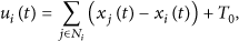
4. Clock Model

Clock synchronization is of significant importance in WSNs. Before delving into the details of synchronizing clocks, we first define some terminologies used in this paper. $c(t)$ denotes a reference clock, where t is the real time, that is, coordinated universal time (UTC). Every sensor node maintains its own local clock, which is a monotonically nondecreasing function of t. This local clock is an ensemble of hardware and software components, essentially a timer that counts the oscillations of a quartz crystal running a particular frequency. In general, the timer is programmed to generate an interrupt, which is called a clock tick. At each clock tick, the interrupt procedure increments the clock value stored in memory.

For any two nodes' local clocks $c_i(t)$ and $c_k(t)$ , the clock $c_i(t)$ is considered correct at time t if $c_i(t)=c(t)$ , or the clock $c_i(t)$ is considered accurate at time t if $d{c}_i(t)/dt=dc(t)/dt$ , and two clocks $c_i(t)$ and $c_k(t)$ are synchronized at time t if $c_i(t)=c_k(t)$ . The aforementioned definitions show that the two synchronized clocks are not always correct or accurate; time synchronization is not related to time correctness and accuracy. As for most applications in WSNs, it is sufficient to achieve clock synchronization. Since the oscillator frequency is time varying due to ambient conditions such as temperature changes, variations of electric supply voltage, and air pressure, clock $c_i(t)$ of node i can be modeled as

$$\begin{array}{cc}& c_i\left(t\right)=k_{i}t+b_i,\end{array}$$

(19)

where $b_i$ is the clock offset, the difference between the time reported by clock $c_i(t)$ and the real time at the initial instant $t_0$ (i.e., $b_i=c_i(t_0)-c(t_0)$ ), and $k_i$ is defined as the skew of the clock $c_i(t)$ . To achieve perfect synchronization in a sensor network, all nodes $i=\mathrm{1,2},\dots ,N$ must precisely compensate for their clock parameters $k_i$ and $b_i$ so that all clocks have zero offset error and all tick at the same rate.

5. TSMA Method

In this section, we present our time synchronization algorithm, that is, TSMA. Instead of trying to synchronize to an external reference like absolute time or UTC, the TSMA method aims to achieve an internal consensus within the network on what time is, and how fast it travels. In every synchronization round, the TSMA algorithm updates the compensation parameters for each node and over time the network clocks converge to a consensus,

$$\begin{array}{cc}& \underset{\text{t}\to \infty }{\lim }{c}_i^{\prime }\left(t\right)=c_c\left(t\right),\end{array}$$

(20)

where $c_c(t)$ is the consensus clock.

The consensus clock is not a physical clock, it is a new virtual clock, that is, generated from the network of nodes running the TSMA algorithm. The consensus clock has its own skew rate and offset relative to the absolute time.

By expanding the clock functions from both sides of (20), we can see the compensation parameters that all nodes must obtain in order to synchronize to the consensus clock,

$$\begin{array}{cc}& \underset{t\to \infty }{\lim }\left(k_i^{\prime }{c}_i\left(t\right)+b_i^{\prime }\right)=k_{c}t+b_c,\\ \underset{t\to \infty }{\lim }\left(k_i^{\prime }{k}_{i}t+k_i^{\prime }{b}_i+b_i^{\prime }\right)=k_{c}t+b_c.\end{array}$$

(21)

Then, we have

$$\begin{array}{cc}& \underset{t\to \infty }{\lim }{k}_i^{\prime }=\frac{k_c}{k_i},\\ \underset{t\to \infty }{\lim }{b}_i^{\prime }=b_c-k_i^{\prime }{b}_i.\end{array}$$

(22)

To achieve these compensation parameters, nodes repeat the TSMA algorithm in synchronization rounds which consist of two main tasks; skew compensation and offset compensation. In skew compensation, the nodes iteratively select the max skew rate estimation from its neighbors in order to improve their skew compensation parameter. In the offset compensation phase, nodes average their neighbors' clock readings to synchronize nodes to a common time.

5.1. Skew Compensation

The goal of skew compensation is to ensure all compensated clocks in the network tick at the same rate, that is,

$$\begin{array}{cc}& \underset{t\to \infty }{\lim }{k}_i^{\prime }{k}_i=k_c,\hspace{1em}\forall i.\end{array}$$

(23)

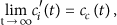
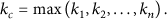
We use max consensus protocol to compensate for clock skew. For perfect skew compensation, the skew rate of the consensus clock is given by

$$\begin{array}{cc}& k_c=\max \left(k_{\mathrm{1}},k_{\mathrm{2}},\dots ,k_n\right).\end{array}$$

(24)

Nodes execute the following algorithm to converge their clock skew to the consensus value.

Step 1. Before running the synchronization algorithm, nodes set their skew estimation $k_i^{\prime }$ to 1, and set their respect life time ${\text{life}}_i$ to $\mathrm{0}$ .

Step 2. At the beginning of each synchronization round, every node increases their own life time ${\text{life}}_i$ by 1. If node i's life time ${\text{life}}_i>3$ , then node i broadcasts a synchronization packet containing its own local clock value ${\tau }_i$ and estimated skew $k_i^{\prime }$ using a CSMA/CA MAC scheme once per synchronization round. Like other synchronization techniques, MAC layer timestamping is required to ensure that clock values are transmitted instantly.

Step 3. If node i receives a synchronization packet from node j at time t, then this node should immediately record its own local time ${\tau }_i(t)$ and node j's information $({\tau }_j(t),k_j^{\prime }(t))$ . If node i has not stored a history local time pair before, then create the local time pair $({\tau }_i(\text{old}),{\tau }_j(\text{old}))$ and assign it with

$$\begin{array}{cc}& \left({\tau }_i\left(\text{old}\right),{\tau }_j\left(\text{old}\right)\right)=\left({\tau }_i\left(t\right),{\tau }_j\left(t\right)\right).\end{array}$$

(25)

If the history local time pair has already existed, and satisfies $k_i^{\prime }(t)*({\tau }_j(t)-{\tau }_j(\text{old}))>k_j^{\prime }(t)*({\tau }_i(t)-{\tau }_i(\text{old}))$ , we will update this node's estimated skew $k_i^{\prime }$ and the history local time pair $({\tau }_i(\text{old}),{\tau }_j(\text{old}))$ using

$$\begin{array}{cc}& k_i^{\prime }\left(t\right)=k_j^{\prime }\left(t\right)*\frac{{\tau }_i\left(t\right)-{\tau }_i\left(\text{old}\right)}{{\tau }_j\left(t\right)-{\tau }_j\left(\text{old}\right)},\\ \left({\tau }_i\left(\text{old}\right),{\tau }_j\left(\text{old}\right)\right)=\left({\tau }_i\left(t\right),{\tau }_j\left(t\right)\right).\end{array}$$

(26)

5.2. Offset Compensation

After the skew compensation algorithm is applied, all local estimators will eventually have the same drift, that is, they will run at the same speed. At this point, it is only necessary to compensate for possible offset errors. To achieve this, each node aims to accurately estimate the instantaneous average time of all its neighbors' clock in the network and set their clocks to this time. From Theorem 5, we can see that every node in the network will finally reach the same status,

$$\begin{array}{cc}& \stackrel{-}{b}\left(t\right)=\frac{\mathrm{1}}{\left|N_i\right|}\sum _{j\in N_i}{b}_j\left(t\right).\end{array}$$

(27)

In reality, however, it is not practically possible for nodes to calculate the instantaneous global average time of all its neighbors' clock in the network. Since sensor networks may consist of a large number of nodes, and one node may have lots of neighbors. It is impossible for nodes to exchange clock values instantaneously, and nodes may suffer from packet loss and other network dynamics.

Instead, the TSMA algorithm converges network clocks to an approximation of $\stackrel{-}{b}(t)$ using the locally available information within the single-hop transmission range of each node. Nodes execute the following algorithm to converge their clock offset to the consensus value.

Step 1. Before running the synchronization algorithm, nodes set their offset estimation $b_i^{\prime }$ to their current local time and set their respect life time ${\text{life}}_i$ to $\mathrm{0}$ .

Step 2. At the beginning of each synchronization round, nodes reset their confidence parameter ${\text{Conf}}_i$ to 1 and increase their life time ${\text{life}}_i$ by 1. If node i's life time ${\text{life}}_i>3$ , then node i broadcasts a synchronization packet containing its estimated offset $b_i^{\prime }$ and confidence parameter ${\text{Conf}}_i$ using a CSMA/CA MAC scheme once per synchronization round. MAC layer timestamping is required to ensure that clock values are transmitted instantly.

Step 3. For each broadcast, all other nodes within receiving range update their own clocks by combining this value with their own clocks using the confidence weighted running average equation and then increase their confidence parameter ${\text{Conf}}_i$ by 1,

$$\begin{array}{cc}& b_i^{\prime }\left(t\right)=\{\begin{array}{cc}{b}_j^{\prime }\left(t\right),\hfill & \text{if}\mathrm{\hspace{0.17em}\hspace{0.17em}}\text{lif}{\text{e}}_i=\mathrm{1}\hspace{0.17em}\hfill \\ \frac{\text{Con}{\text{f}}_i\left(t\right)*b_i^{\prime }\left(t\right)+\text{Con}{\text{f}}_j\left(t\right)*b_j^{\prime }\left(t\right)}{\text{Con}{\text{f}}_i\left(t\right)+\text{Con}{\text{f}}_j\left(t\right)},\hfill & \text{if}\mathrm{\hspace{0.17em}\hspace{0.17em}}\text{lif}{\text{e}}_i>\mathrm{1},\hfill \end{array}\\ \text{Con}{\text{f}}_i\left(t\right)=\text{Con}{\text{f}}_i\left(t\right)+\mathrm{1}.\end{array}$$

(28)

The confidence parameters give weighting to the clock values from nodes that have already received synchronization packets in the current round. These nodes are generally closer to a local consensus than those who have not received any sync packets, and this was found to increase the rate of convergence.

6. Simulation

In this paper, we use max consensus to compensate for clock skew and use average consensus to compensate for clock offset. To show the correctness and robustness of the TSMA algorithm, we make a simulation in MATLAB; the following is the simulation environment: there are 100 WSN nodes in the $10*10$ grid, one grid one node, and we place the node in the center of the grid, the base value of nodes' oscillator is 32.768 KHz, the skew rates are assigned randomly from a normal distribution with mean = 1 and standard deviation = 20 PPM, nodes are given an initial error distribution between 0 and 1000 ticks.

6.1. Offset Compensation

In this simulation, we set the time synchronization period to 1 minute. Nodes broadcast one sync packet per round in random order with a transmission range of 2, which means if the distance between two nodes is less than 2, then they can communicate with each other. Figure 1 shows the clock errors from average time measured in clock cycles. In the first three synchronization periods, nodes' life time is less than 3, so they do not transmit any synchronization packet to their neighbors, and then in 3 minutes, nodes start to compensate for the clock skew and offset. After seven rounds compensation, 100 nodes in the network achieve the synchronization state, the synchronization error between any two nodes is included between ±10 ticks.

Figure 1

Clock error of 100 simulated nodes running the TSMA protocol in a $10*10$ network with synchronization period of 1 min and transmission range of 2.

The geographic distribution of clock errors in the network is shown in Figure 2. It can be seen that before Figure 2(a), the first round of offset compensation, the clock error relative to the average time can reach up to 550 ticks, but after Figure 2(b), the first round offset compensation, the clock error reduces to 140 ticks. Also we can see that the clock error after compensation transfer smoothly in geographic distribution, the local error between any neighboring nodes is no larger than 50 ticks.

Figure 2

Geographic distribution of synchronization error of a $10*10$ sensor network for transmission range of 2 (a) before and (b) after one round of offset compensation.

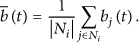
A histogram of the clock errors is shown in Figure 3. It can be seen that before Figure 3(a), the first round of offset compensation, the standard deviation of clock error reaches up to 286.32, but after Figure 3(b), the first round of offset compensation, this value reduces to 70.90. From Figures 2 and 3, we can see that after the first round of offset compensation, the clock errors among nodes are significantly reduced.

Figure 3

Histogram of the synchronization errors from the instantaneous global average time of the sensor network (a) before and (b) after one round of offset compensation.

Figure 4 shows the convergence of the skew rates of 100 nodes in this simulation. From Figure 4, we can see that after two synchronization periods all the 100 nodes' skew rates converge on the maximum clock skew.

Figure 4

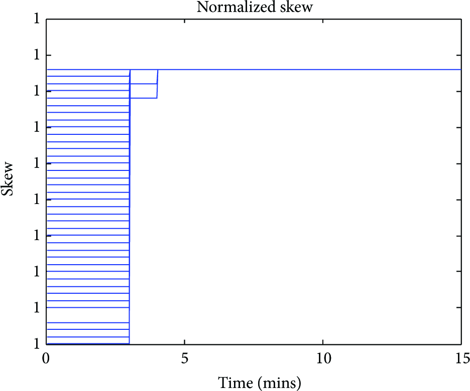
Convergence of the skew rate of 100 simulated nodes running the TSMA protocol in a $10*10$ network with synchronization period of 1 min and transmission range of 2.

6.2. Transmission Range

Figure 5 shows the transmission range's effect to algorithm performance. We set the transmission range to 1, 2, and 3, respectively, then compare their convergence speed with each other. From Figure 5, we can see that synchronization accuracy and convergence speed are found to improve as the transmission range of the nodes increased, since nodes could receive synchronization packets from a greater proportion of the network population. On the other side, to increase the transmission range, we also increase the energy consumption of nodes, so in the practical application, we should make a tradeoff between energy consumption and convergence speed.

Figure 5

Clock errors of 100 simulated nodes running the TSMA protocol in a $10*10$ network with synchronization period of 1 min in transmission ranges of 1 (a), 2 (b), and 3 (c).

6.3. Dynamic Topology

The simulation, shown in Figure 6, is intended to study the robustness properties of the TMSA protocol subject to node failure and node replacement, as well as the performance in terms of convergence speed and steady state synchronization error. The synchronization period is set to 1 minute which is sufficiently large to exhibit the effects of different clock speeds. The simulation was run for about 50 minutes and presents 4 different regions of operation indicated by the letters A, B, C, and D which model potential node failure or the addition of the new nodes. In Region A, all nodes are turned on simultaneously with random initial conditions of their local clocks. After 2 synchronization periods, the synchronization error between any two nodes is included between ±10 ticks, that is, the maximum error is smaller than 20 ticks. At the beginning of Region B, about 20% of the nodes chosen random in the grid are switched off and then switched on at different random times. Once a node is switched on, it starts updating its estimated time using TSMA protocol but does not transmit any message for the first three synchronization periods to avoid injecting large disturbances into the already synchronized network, and then it starts to transmitting and receiving messages equally. The plot in Figure 6 clearly shows that the nodes get synchronized as soon as they are turned on without perturbing the overall network behavior. At the beginning of Region C, about 20% of the nodes turned off their radio, that is, they stop updating their parameters $k^{\prime }$ , $b^{\prime }$ , then we turn on the 20% nodes' radio at about 35 minutes. In this procedure, we can see that all nodes keep the synchronized state, the reason is that their skew rates have already converged to the maximum skew rate in the network, these 20% nodes still synchronize with others. At the beginning of Region D, we replace the node in the top left corner with one node having 40 PPM drift, which is the max skew rate in the network now, and then all the other nodes will compensate themselves to this skew value. From Figure 6, we can see that three synchronization period after the new node joining the network, it starts to transmitting messages to its neighbors, after a short transient the nodes quickly synchronize again.

Figure 6

Clock errors of 100 simulated nodes running the TSMA protocol in a $10*10$ network with synchronization period of 1 min and transmission range of 3. Region A: all nodes are on. Region B: 20% of the nodes are turned off and then turned on at random times. Region C: 20% of the nodes turned off their radio, and then turned on their radio after 5 synchronization periods. Region D: replace the node in the top left corner with one node having 40 PPM drift.

7. Conclusions

This paper presented a new synchronization algorithm for WSN, the time synchronization using consensus protocol, which is based on consensus algorithms whose main idea is to average local information to achieve a global agreement on a specific quantity of interest. The proposed algorithm is fully distributed, asynchronous, includes skew compensation, and is computationally light. Moreover, it is robust to dynamic network topologies due, for example, to node failure or replacement. Finally, a set of simulations are presented to show the good performance of the proposed protocol. However, extensive work is still necessary to compare the performance of our proposed approach relative to FTSP [3] and other protocols over large scale multihop sensor network and over longer periods.