Sage Journals: Discover world-class research

Abstract

Current deterministic sensor deploying methods always include the uncovered space greedily to reduce the number of deployed sensors. Because the sensing area of each sensor is circle-like, these greedily methods often divide the region of interest to multiple tiny and scattered regions. Therefore, many additional sensors are deployed to cover these scattered regions. This paper proposes a Jigsaw-based sensor placement (JSP) algorithm for deploying sensors deterministically. Sensors are placed at the periphery of the region of interest to prevent separating the region of interest to isolated regions. An enhanced mechanism is also proposed to improve the time complexity of the proposed method. The scenarios with and without obstacles are evaluated. The simulation results show that the proposed method can cover the whole region of interest with fewer deployed sensors. The effective coverage ratio of JSP method is less than 2. It is better than the maximum coverage method and the Delaunay triangulation method. The deploying sensors have more efficient coverage area, and the distribution of the incremental covered area is close to normal distribution.

1. Introduction

Sensor networks are applied for monitoring environment. Sensors are similar to the guard men standing at the specific locations for scouting. Usually, sensors have the wireless communication components to deliver their collected data back to the sink, which is a data collector in the network. Sensors can be deployed in the field for the environmental habitat monitoring [1], the natural hazards monitoring [2], the forest-fire detection [3], or the nuclear radiation detection [4]. Sensors are also used in the medical center to quicken the emergency response [5, 6]. Deployed sensors can also be used for localizing the users [7] or detecting the temperature of devices [8].

The placement of sensor nodes can be deterministic or random. The random deployment cannot guarantee the region of interest completely covered by the deployed sensors. Thus, more sensors need to be deployed to include the uncovered space [9, 10]. Giving the mobile ability for sensors to adjust their initial positions is the common used solution [11, 12]. The deterministic deploying methods consider covering the whole region of interest in the first time that sensors are deployed [13–17]. The object is determining the locations of sensors to minimize the number of deployed sensors. Finding minimum number of sensors to cover the whole space is an NP-complete problem similar to the coloring problem in a graph. Thus, finding a polynomial time solvable problem to approximate the optimal solution is the object of this research problem. The existing methods always greedily place a sensor to the place that can cover the largest uncovered space. So, the number of deployed sensors can be reduced. However, the sensing area of a sensor is circle-like. Using greedy methods to cover the whole region of interest introduces multiple small isolated regions. Sensors must be deployed in these scattered regions to achieve full coverage. Therefore, more sensors are deployed.

This paper proposes an enhanced deterministic deploying method named as the Jigsaw-based sensor placement (JSP) algorithm. Sensors are deployed from the periphery of the region of interest such as solving the jigsaw puzzle. The proposed JSP algorithm can prevent introducing the isolated regions. The open-space scenario and center obstacle scenario are evaluated. The JSP can use fewer numbers of sensors to cover the region of interest. The overlapping coverage between sensors can also be reduced.

The rest of this paper is organized as follows. The related studies are reviewed in Section 2. Section 3 gives the main idea of JSP and the methodology to reduce the time complexity of JSP. The evaluation results are shown in Section 4. Finally, the conclusion is given in Section 5.

2. Related Works

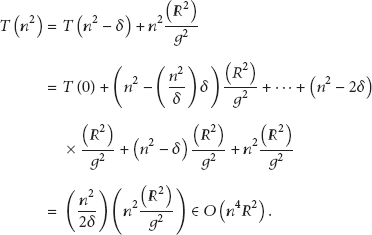
The deterministic deploying methods focus on using minimum numbers of sensors to cover the whole region of interest. Dhillon et al. presented two methods, called as MAX_AVG_COV and MIN_AVG_COV [13, 14]. The region of interest is divided into $n \times n$ grids, and an $n^{2} \times n^{2}$ matrix is used to represent the detection probability between any two grids. Each grid g is scored by accumulating the probabilities of all neighbor grids covered by a sensor centered at g. The MAX_AVG_COV method chooses the highest score grid as the candidate position to place the next sensor. After a sensor is placed, the matrix is updated. The procedure continues until all grids are covered.

The MAX_AVG_COV method scans all grids and computes their scores. The time complexity to determine the deploying location is $O (n^{4})$ . In a large deploying area, the computation overhead on scoring the grids is enormous. In addition, reducing the grid size also generates high computation overhead. Greedily placing the next sensor at the location which can include the most uncovered space will introduce many small isolated regions as shown in Figure 1 and each isolated region needs a sensor to cover it. To prevent placing addition sensors on the tiny isolated regions, the MIN_AVG_COV method is proposed. The candidate uncovered grid to place the next sensor is the one which can include minimum uncovered space. MIN_AVG_COV method is proposed to prevent generating the isolated region, but the cost is to deploy more sensors. Xu and Sahnialso proposed a greedy method as the MIN_AVG_COV but using the integer linear programming formulation to find the minimum cost position for deploying of sensors [15] with heterogeneous sensors.

Figure 1

The generated isolated regions in greedy deployed methods.

Wu et al. proposed a DT-Score algorithm [16] which utilizes the Delaunay triangulation to determine the location for placing sensors. The DT-Score algorithm consists of two phases. In the first phase, the sensors are placed along the contour of the boundary and the obstacles to eliminate the coverage holes are generated near them. All grids in the region of interest are scanned to identify the contours of the obstacles. The time complexity of this phase is $O (n^{2})$ . The second phase is to refine the deployment. New candidate positions to place sensors are the centers of the circumcircle of all triangles generated through the Delaunay triangulation algorithm. All candidate points are scored, and the next sensor is placed at the location which gets the most coverage gains. The Delaunay triangulation algorithm is applied to add vertices one by one continuously to include the uncovered space so that the time complexity to triangulate the graph is $O (m^{3})$ . The m is the number of sensors deploying along the contour of obstacles. After that the DT-Score algorithm needs $O (n^{2} \log n)$ time complexity to obtain the candidate location for the placing sensors. The procedure is repeated until the predefined number of deployable sensors is reached.

At first, the DT-Score algorithm computes the centers of the circumcircles of the triangles generated by the Delaunay triangulation algorithm as the candidate positions. The center of the circum-circles with maximum radius is the position to place the next sensor. It also generates multiple scattered isolated regions as the MAX_AVG_COV method. The sensors placed near the obstacles only slightly moderated this problem. Therefore, Dhillon et al. also proposed the MIN_AVG_COV method for reducing the isolated regions. The MIN_AVG_COV method always places the next sensor at the location which includes the least uncovered space. The number of deployed sensors is also worse than MAX_AVG_COV. However, it gives the motivation to improve the deterministic deploying methods. If sensors can be added one by one from the periphery of the uncovered space, the probability to generate an isolated region will be reduced. It is similar to the strategy of playing a Jigsaw puzzle game. A similar method is proposed in [17] by considering a different coverage ratio.

3. The Jigsaw-Based Sensor Placement (JSP) Algorithm

3.1. Basic JSP Algorithm

Assume all sensors have the same sensing radius R. V is the set containing all uncovered grids in the region of interest. The set $B \in V$ includes all boundary grids. Similar to the MAX_AVG_COV method, the region of interest is divided into $n \times n$ grids. Each grid $P_{i j}$ is initially assigned a token T which is used for computing the score of each grid. The value of T is set as

\begin{matrix} T (P_{i j}) = {\begin{cases} 0, & otherwise \\ 1, & P_{i j} \in B, \end{cases} {i, j} = [1 \dots n] . \end{matrix}

(1)

Let $C_{i j}$ be the set containing all grids which are covered by the sensor centered at $P_{i j}$ . Thus, the grids $P_{x y}$ included by $C_{i j}$ must satisfy $| \bar{P_{x y} P_{i j}} | < R$ . The score of $P_{i j}$ is the accumulated tokens of the grids in $C_{i j}$ . We can represent it as

\begin{matrix} S (P_{i j}) = \sum_{\forall P_{x y} \in C_{i j}} T (P_{x y}), {x, y} = [1 \dots n] . \end{matrix}

(2)

And the next candidate grid to place a sensor will be the one which has the highest score:

\begin{matrix} P^{*} = \max {S (P_{i j})} . \end{matrix}

(3)

After placing a sensor at the grid $P^{*}$ , the grids $g \in C_{i j}$ are removed from V. The set B is also updated for refreshing the boundary. The deploying procedure continues until all elements in V are exhausted. The scoring algorithm is given in Algorithm 1.

Algorithm 1: The scoring algorithm of the JSP.

(1) V: The set of uncovered grids

(2) B: The set of the boundary grids

(3) $P^{*}$ : The highest score grid

(4) $T (P_{i j})$ : Token of a grid point

(5) R: Sensing radius of a sensor node

(6) //Initial

(7) For all $P_{i j} \in V$

(8) If $P_{i j} \notin B$ then

(9) set $T (P_{i j}) = 0$

(10) Else

(11) set $T (P_{i j}) = 1$ , add $P_{i j}$ into B

(12) End

(13) //Scoring

(14) Do while V is not empty

(15) Use (2) to compute the score of $P_{i j} \in V$

(16) Get the highest score $P^{*}$ and place a sensor in it, remove $P^{*}$ from V

(17) For all $P_{i j} \in V$

(18) Case: $| P^{*} P_{i j} | < R$

(19) Set $T (P_{i j}) = 0$

(20) Remove $P_{i j}$ from V

(21) Case: $| P^{*} P_{i j} | = R$

(22) Set $T (P_{i j}) = 1$

(23) Add $P_{i j}$ into B

(24) End

(25) If $P_{i j} \notin V$

(26) Remove $P_{i j}$ from B

(27) End

The time complexity of JSP is also proportional to the number of grids. Let the grid size be $g^{2}$ . All grids in V need to be scored. Each grid requires scanning the rectangle that includes the sensing area of a sensor to accumulate the tokens. The rectangle is $(R^{2} / g^{2}) \in O (R^{2})$ area. The initial number of grids in set V is $n \times n$ and decreases after sensors are deployed. The average grid decreasing rate in V, denoted as δ, is ranged from 1 to $R^{2} / g^{2}$ . The time complexity can be represented as the recursive relation, $T (n^{2})$ . The time complexity is $O (n^{4} R^{2})$ . Consider the following:

\begin{array}{l} T (n^{2}) = T (n^{2} - δ) + n^{2} \frac{(R^{2})}{g^{2}} \\ = T (0) + (n^{2} - (\frac{n^{2}}{δ}) δ) \frac{(R^{2})}{g^{2}} + \dots + (n^{2} - 2 δ) \\ \times \frac{(R^{2})}{g^{2}} + (n^{2} - δ) \frac{(R^{2})}{g^{2}} + n^{2} \frac{(R^{2})}{g^{2}} \\ = (\frac{n^{2}}{2 δ}) (n^{2} \frac{(R^{2})}{g^{2}}) \in O (n^{4} R^{2}) . \end{array}

(4)

A little example is given in Figure 2 to show the operation of the JSP algorithm. Initially, all boundary grids are set to 1 and others are set to 0 as shown in Figure 2(a). Next, each grid is rescored according to the number of included boundary grids if a sensor is placed in it. As the grid (4, 3) in the Figure 2(b), it includes the boundary grids (1, 2), (1, 3), (1, 4), (1, 5), and (1, 6). So, its score is 5 (note that a grid is counted as included if more than two-thirds of the grids are covered by the sensor). Figure 2(b) shows that four grids (3, 3), (6, 3), (3, 6), and (6, 6) have the highest score 9, and the first one (3, 3) is selected as the next candidate position to place a sensor.

Figure 2

An example of the JSP algorithm.

As a sensor is placed at (3, 3), the grids covered by sensor is marked covered. The boundary grids covered by sensor is removed, and the grids located on the edge of the sensor coverage will be marked as new boundary grids as shown in Figure 2(c). Then, all uncovered grids will be re-scored as shown in Figure 2(d). The selected grid with the highest score is the (3, 6). After the next sensor is placed, covered grids are marked and new boundary grids are selected as shown in the Figure 2(e). This procedure is performed until all grids are covered. In this example, the final positions to place sensors will be (3, 3), (6, 3), (3, 6), and (6, 6).

3.2. Improved JSP Algorithm

In Algorithm 1, all grids in the set V are scanned to update the score value after a sensor S is deployed. However, only those grids near the deployed S need to be rescored instead of all grids in V . As the example in Figure 3, the sensor S is placed at the grid X. Those grids covered by S set their scores to zero. The grids in the coverage edge of S become the new boundary. The uncovered grid whose minimum distance to the boundary grids is less than R should update its score. The grids to refresh their score will be the ones whose locations are within the circle $C_{out}$ centered at grid X with radius $2 R$ but not in the circle $C_{in}$ centered at grid X with radius R. The area size is ${3 R}^{2} π$ . To simplify the computation, the area included by the rectangle center at X bound to the circle $C_{out}$ but not included in the rectangle center at X with edge length $\sqrt{2} R$ is scanned and thus, the scan area will be $(2 R)^{2} - ((\sqrt{2} / 2) R)^{2} = 3.5 R^{2}$ . Therefore, $T (n^{2})$ can be represented as

\begin{matrix} T (n^{2}) = T (0) + (3.5 R^{2}) R^{2} + \dots + (3.5 R^{2}) R^{2} + n^{2} R^{2} \\ = (\frac{n^{2}}{δ} - 1) (3.5 R^{2}) R^{2} + n^{2} R^{2} \\ = (\frac{n^{2}}{δ}) (3.5 R^{2}) R^{2} - 3.5 R^{2} + n^{2} R^{2} \in O (n^{2} R^{4}) . \end{matrix}

(5)

Figure 3

The rescoring area after a sensor node deployed.

By limiting the area to update score, JSP can effectively reduce the time complexity from $O (n^{4} R^{2})$ to $O (n^{2} R^{4})$ . The time complexity is $O (n^{2})$ which is better than $O (n^{2} \log n)$ of the DT-Score [16]. We will prove that JSP can use fewer numbers of deployed sensors than the DT-Score method in the simulation section. The enhanced JSP algorithm is given in Algorithm 2.

Algorithm 2: The enhanced JSP algorithm.

(1) V: the set of uncovered grid points

(2) B: the set of the boundary grid points

(3) $V^{*}$ : the set of uncovered grid points within the circle centered at $P^{*}$

(4) $P^{*}$ : the grid with maximal score

(5) //initial

(6) For all $P_{i j}$ in V {

(7) If $P_{i j}$ is not a boundary point then

(8) set $T (P_{i j}) = 0$

(9) Else

(10) set $T (P_{i j}) = 1$ , add $P_{i j}$ into B

(11) }

(12)

(13) //scoring

(14) Computes the $S (P_{i j})$ of each $P_{i j}$ in V according to (2)

(15) Use maximal heap tree to maintain sorting results of $S (P_{i j})$ in V

(16) Place the sensor at $P^{*}$

(17) Do While (V is not empty) {

(18) For all $P_{i j}$ in $V^{*}$ {

(19) Case: $| P^{*} P_{i j} | < R$

(20) Set $T (P_{i j}) = 0$

(21) Remove $P_{i j}$ from V

(22) Case: $| P^{*} P_{i j} | = R$

(23) Set $T (P_{i j}) = 1$

(24) Add $P_{i j}$ into B

(25) }

(26) Remove the $P_{i j}$ from B if $P_{i j}$ is not in V

(27) Computes the $S_{i j}$ of each $P_{i j}$ in $V^{*}$ according to (2)

(28) Re-heap maximal heap tree, Place the sensor at $P^{*}$

(29) }

4. Simulation Results

This section shows the simulation results. The proposed JSP method is implemented using the C++ program. The MAX_AVG_COV method [13, 14], and the Delaunay triangulation method [16, 17]. The MAX and DT represent the MAX_AVG_COV method and the Delaunay triangulation method in the following figures. The MIN_AVG_COV method is not compared because its result is worse than that of the MAX_AVG_COV method. The evaluation methods include the number of deployed sensors, effective coverage ratio (ECR), and distribution of incremental coverage area (ICA).

The number of deployed sensors evaluates the efficiency of a deterministic deploying method when the size of region of interest is fixed. The method using fewer sensors to cover the region of interest is more efficient. The effective coverage ratio is the ratio that the maximal coverage area generated by all deployed sensors over the area of the region of interest. The method which generates less overlapping area between sensors will have small ECR. The $ECR = 1$ is the ideal case implying no overlapping on sensing area. In the real world, the circle-like sensing area of sensor must be overlapping with others. $ECR = 1$ can only be used as the reference value to evaluate the deploying methods. The ICA is the area which is covered for first time after S has been placed. The results are represented as the percentage of the sensing area of a sensor. There are ten scales to evaluate this area size. They are 0%–10%, 10%–20%,…, and so on. The distribution of ICA can evaluate the deploying efficiency.

4.1. Environment Setup

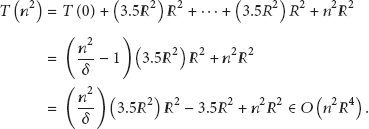
In our simulation, the region of interest is $400 m \times 400 m$ . The grid size is 1 m². Three scenarios are simulated as shown in Figure 4. The first scenario is an open-space. No obstacle is in the region of interest. The second scenario has a $200 m \times 200 m$ rectangle obstacle in the center of the region of interest, and the third scenario has multiple obstacles irregularly placed in it. In each scenario, sensors with sensing radius 20 m, 30 m, 40 m, and 50 m are simulated. The sensing coverage of each sensor is assumed to be a perfect circle. The deploying procedure finishes when all grids in the simulation area are covered.

Figure 4

The simulation scenarios.

4.2. Numerical Results

Figure 5 shows the number of sensors deployed to cover the whole space. The OPT represents the ideal case which simply divides the whole area size of the region of interest by the coverage area of a sensor. Because the sensing area of a sensor is a circle, the coverage areas of sensors must be overlapped. Thus, no method can use the same number of sensors to cover the whole region of interest as the OPT method. The OPT method is used as the lower bound of the number of deployed sensors.

Figure 5

The number of deployed sensors in both scenarios.

In both simulated scenarios, the MAX method deploys most numbers of sensors to cover the whole space. This method introduces many small isolated regions when it greedily searches the position which can cover the largest uncovered space to place the next sensor. Thus, additional sensors are placed to cover those isolated regions. Increasing the sensing radius does not change the situation of the MAX method. The MAX method still has the worst result in any kind of sensor radius. More than 200 sensors are used to cover the whole space when sensing radius is 20 m in both scenarios.

The number of deployed sensors in the DT method is slightly better than the MAX method in both scenarios. The number of sensors of the DT method is less than the MAX method about 5% to 12% in the open-space scenario and about 10% to 20% in the obstacle scenario. Sensors in DT method are initially deployed along the contour of the region of interest. The DT method needs to add sensors one by one to cover the whole regions. The next location to add a sensor is the center of the circum-circle of the triangulation with the largest radius. Therefore, DT method is also similar to the MAX method that greedily places the next sensor to cover the maximum number of uncovered grids. However, placing the sensors along the boundaries of the obstacles prevents overlapping near the boundary of region and the obstacles. Thus, the results of DT method are better than those of the MAX method.

The JSP method exhibits better results than the MAX and DT methods in both scenarios. The number of deployed sensors of the JSP method is less than the MAX method about 34%–36% in the open-space scenario and about 28%–39% in the obstacle scenario. JSP also greedily includes the uncovered spaces, but it prevents dividing the uncovered space into isolated regions. In the open-space with sensing radius 20 m, JSP only needs 150 sensors to cover the whole space. The number of deployed sensors in the JSP method is about 1.5 times of the sensors used in the OPT method. In the obstacle scenario, the number of deployed sensors is still less than twice of that in OPT. The scenario with multiple obstacles is similar to the center obstacle scenario. More obstacles will also increase the initial deployed sensors of the DT method. More sensors are placed in the contour of the obstacles. As the sensing radius increases, the DT method still needs deployed sensors to enclose the obstacles. Therefore, the number of deployed sensors is close to that in the results of the MAX method.

Figure 6 shows the results of the ECR. The ECR of the OPT method is 1 which is the lower bound. The ECR of the MAX method is higher than 2.2 in both scenarios. In the obstacle scenario with sensing radius 50 m, the ECR of MAX is 3. This result implies that increasing the sensing radius generates more overlapping between sensors. When the space is divided into multiple isolated regions, large sensing radius will worsen the ECR. The ECR of the DT method is 2 in both scenarios. Placing sensors aside, the contour reduces the overlapping coverage near the boundary and obstacles. The ECR of JSP is less than 1.8. It can suppress the ECR even increasing the sensing radius. In the scenario of multiple obstacles, the ECR of DT method in the cases of sensing radius 40 m and 50 m is worse than the MAX method. Large radius causes the initial deployed sensors which enclosed the obstacles to severely overlap their sensing areas with others. Therefore, the ECR is worse than the MAX method.

Figure 6

The effective coverage ratio.

The distribution of ICA in the open-space scenario is shown in Figure 7. In the MAX method, the deployed sensors with ICA less than 20% sensing area are 40%–50% and the number of sensors with ICA more than 90% sensing area is 20%–40% as shown in Figure 7(a). The percentage of sensors with high ICA decreases when the length of sensing radius increases. It is related to the results in Figure 5. The MAX method deploys many sensors to cover the isolated regions.

Figure 7

Distribution of ICA in open-space scenario.

The DT method improves the ICA but still many sensors are deployed to cover the small regions. The 25%–35% deployed sensors have their ICA less than 20% sensing area and 40%–50% sensors have their ICA more than 80% sensing area. Greedily placing the next sensor at the center of the circum-circle of the triangle with maximum radius introduces isolated regions as the MAX method. Deploying sensors near the contour of obstacles only moderates the problem suffered by the MAX method.

For the JSP, approximating 70% deployed sensors have their results on ICA more than 80%. The percentage of the deployed sensors with ICA smaller than 20% is less than 10% in all simulated sensing radii. The fluctuation of the ICA distribution is less than 10% when the sensing radius increases. The ICA with 70%–80% dominates the major portion of the deployed sensors. The results imply that JSP algorithm prevents deploying a sensor for covering a tiny uncovered space.

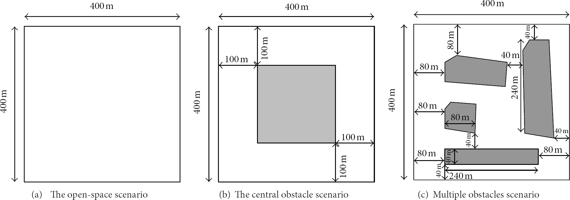
Figure 8 shows the ICA in the obstacle scenario. The distribution is similar to Figure 7. In all compared methods, the distribution of ICA has explicit fluctuations when sensing radius is more than 40 m. Large sensing radius includes more area occupied by the obstacle. Thus, the distribution has great variation. However, the JSP and the MAX can still retain the distribution trend as shown in Figure 7. For the DT method, the obstacle limits the organization of the Delaunay triangulations. Therefore, the DT method exhibits different ICA distribution.

Figure 8

Distribution of ICA in central obstacle scenario.

Figure 9 shows the ICA of the scenario with multiple obstacles. The MAX method and the JSP method still retain the distributions as the Figures 7 and 8. However, the distribution of the DT method has changed. Most of the sensors are used to cover a tiny area. The deploying efficiency of the DT method greatly decays in the scenario with multiple obstacles.

Figure 9

Distribution of ICA in multiple obstacles scenario.

5. Conclusions

This paper proposed a Jigsaw-based sensor deploying (JSP) algorithm for wireless sensor network. Sensors are placed at the periphery of the region of interest. The JSP method prevents dividing the uncovered space into isolated regions and uses fewer numbers of sensors to cover the whole region of interest. The time complexity of the enhanced JSP algorithm is $O (n^{2} R^{4})$ which is better than that in MAX_AVG_COV and not worse than the DT-Score method. The number of deployed sensors of the JSP method is less than the MAX_AVG_COV method about 34%–36% in the open-space scenario and about 28%–39% in the obstacle scenario. The effective coverage ratio of JSP is less than 1.8 instead of more than 2 in the DT-Score and the MAX_AVG_COV. The distribution of incremental coverage area (ICA) is close to normal distribution. Sensors are not deployed to cover tiny regions.

References

Mainwaring

Polastre

Szewczyk

Culler

Anderson

Wireless sensor networks for habitat monitoring

Proceedings of the 1st ACM International Workshop on Wireless Sensor Networks and Applications

September 2002

88 97

2-s2.0-0036986465

Kenney

J. D.

Poole

D. R.

Willden

G. C.

Abbott

B. A.

Morris

A. P.

McGinnis

R. N.

Ferrill

D. A.

Precise positioning with wireless sensor nodes: monitoring natural hazards in all terrains

Proceedings of IEEE International Conference on Systems, Man and Cybernetics (SMC '09)

October 2009

722 727

2-s2.0-74849098550

10.1109/ICSMC.2009.5346714

Zhang

Yin

Liu

Guo

Forest fire detection system based on wireless sensor network

Proceedings of the 4th IEEE Conference on Industrial Electronics and Applications (ICIEA '09)

May 2009

520 523

2-s2.0-70349308495

10.1109/ICIEA.2009.5138260

Qian

Fuller

Chang

Quickest detection of nuclear radiation using a sensor network

Proceedings of IEEE Conference on Technologies for Homeland Security (HST '12)

November 2012

648 653

Gao

Pesto

Selavo

Chen

Lim

Terzis

Watt

Jeng

Chen

B.-R.

Lorincz

Welsh

Wireless medical sensor networks in emergency response: implementation and pilot results

Proceedings of IEEE International Conference on Technologies for Homeland Security (HST '08)

May 2008

187 192

2-s2.0-50649083511

10.1109/THS.2008.4534447

Tsou

Y.-L.

Berber

Design, development and testing of a wireless sensor network for medical applications

Proceedings of the 7th International Wireless Communications and Mobile Computing Conference (IWCMC '11)

July 2011

826 830

2-s2.0-80052510462

10.1109/IWCMC.2011.5982653

Tsai

Y.-R.

Tsai

Y.-J.

Sub-optimal step-by-step node deployment algorithm for user localization in wireless sensor networks

Proceedings of IEEE International Conference on Sensor Networks, Ubiquitous, and Trustworthy Computing (SUTC '08)

June 2008

114 121

2-s2.0-50949100876

10.1109/SUTC.2008.33

Wang

Xing

Chen

Lin

C.-X.

Chen

Towards optimal sensor placement for hot server detection in data centers

Proceedings of the 31st International Conference on Distributed Computing Systems (ICDCS '11)

July 2011

899 908

2-s2.0-80051882727

10.1109/ICDCS.2011.20

Hassanein

Takahara

Wang

Differential random deployment for sensing coverage in wireless sensor networks

Proceedings of the Global Telecommunications Conference (GLOBECOM '06)

December 2006

1 5

2-s2.0-50949104297

10.1109/GLOCOM.2006.483

10.

Hassanein

Takahara

Wang

Relay node deployment strategies in heterogeneous wireless sensor networks

IEEE Transactions on Mobile Computing 2010 9 2 145 159

2-s2.0-73949127423

10.1109/TMC.2009.105

11.

Salehizadeh

S. M. A.

Dirafzoon

Menhaj

M. B.

Afshar

Coverage in wireless sensor networks based on individual particle optimization

Proceedings of the International Conference on Networking, Sensing and Control (ICNSC '10)

April 2010

501 506

2-s2.0-77953087357

10.1109/ICNSC.2010.5461607

12.

Huang

S.-C.

Ion-6: a positionless self-deploying method for wireless sensor networks

International Journal of Distributed Sensor Networks 2012 2012 10

2-s2.0-84855275485

10.1155/2012/940920

940920

13.

Dhillon K

S. S.

Chakrabarty

Placement for effective coverage and surveillance in distributed sensor networks

Proceedings of IEEE International Conference on Wireless Communications and Networking (WCNC '03)

March 2003

1609 1614

14.

Dhillon

S. S.

Chakrabarty

Iyengar

S. S.

Sensor placement for grid coverage under imprecise detections

Proceedings of the 5th International Conference on Information Fusion

July 2002

1581 1587

15.

Sahni

Approximation algorithms for sensor deployment

IEEE Transactions on Computers 2007 56 12 1681 1695

2-s2.0-36348979444

10.1109/TC.2007.1063

16.

C.-H.

Lee

K.-C.

Chung

Y.-C.

A Delaunay triangulation based method for wireless sensor network deployment

Proceedings of the 12th International Conference on Parallel and Distributed Systems (ICPADS '06)

July 2006

253 260

2-s2.0-34047208114

10.1109/ICPADS.2006.11

17.

Zhu

Sensor node optimal placement algorithm based on coverage rates

Proceedings of the International Conference on Computer Science and Service System (CSSS '11)

June 2011

2547 2550

2-s2.0-80052331102

10.1109/CSSS.2011.5972209

A Jigsaw-Based Sensor Placement Algorithm for Wireless Sensor Networks

Abstract

1. Introduction

2. Related Works

3. The Jigsaw-Based Sensor Placement (JSP) Algorithm

3.1. Basic JSP Algorithm

Algorithm 1: The scoring algorithm of the JSP.

3.2. Improved JSP Algorithm

Algorithm 2: The enhanced JSP algorithm.

4. Simulation Results

4.1. Environment Setup

4.2. Numerical Results

5. Conclusions

References