A Rough Set Approach of Mechanical Fault Diagnosis for Five-Plunger Pump

Abstract

Five-plunger pumps are widely used in oil field to recover petroleum due to their reliability and relatively low cost. Petroleum production is, to a great extent, dependent upon the running condition of the pumps. Closely monitoring the condition of the pumps and carrying out timely system diagnosis whenever a fault symptom is detected would help to reduce the production downtime and improve overall productivity. In this paper, a rough set approach of mechanical fault diagnosis is proposed to identify the five-plunger pump faults. The details of the approach, together with the basic concepts of the rough sets theory, are presented. The rough classifier is a set of decision rules derived from lower and upper approximations of decision classes. The definitions of these approximations are based on the indiscernibility relation in the set of objects. The spectrum features of vibration signals are abstracted as the attributes of the learning samples. The minimum decision rule set is used to classify technical states of the considered object. The diagnostic investigation is done on data from a five-plunger pump in outdoor conditions on a real industrial object. Results show that the approach can effectively identify the different operating states of the pump.

1. Introduction

In many fields of nature science, society science, engineering, and so forth, there are many uncertain and imperfect data needed to be processed. The data collected from the real systems usually include not only useful information but also noisy data. That is, they are inaccurate, even incomplete. It is not practical to just eliminate or dodge this uncertainty by using some hypothesis mathematically. On the contrary, over the past decades many theories and techniques have been developed to deal with incompleteness and uncertainty in information analysis scientifically. Among them, the most successful ones are fuzzy set theories [1, 2] and the Dempster-Shafer evidence reasoning [3, 4]. However, additional information and prior knowledge are needed when they are used to solve some problems. For example, the membership functions are determined by experience and judgement of the experts in certain fields, and the basic probability assignment and statistical probability are sometimes not easy to be obtained, which means that the treatment of the uncertain information of the running conditions of the pump, to some extent, is subjective. In 1982, Pawlak, a Poland researcher, presented the rough sets theory [5] which is a mathematical tool depicting the imperfectness and uncertainty. It can analyze the imprecise, inconsistent, and incomplete information effectively. It can also process the data and also reason and mine the knowledge implied in the data to reveal the potential laws. This theory has strong practicability. Having been studied and developed for more than 20 years, it has great progress both in theoretical and practical application. Rough sets have been used in the areas of inductive reasoning, number logic analysis and redact, building predictive model, decision support, process control, machine learning, database mining, automatic classification, pattern recognition, and so forth.

Five-plunger pump is widely used in oil field to recover petroleum due to its reliability and relatively low cost. It is a typical reciprocating machinery, consisting of many rotating and back-forth motion parts. Diagnosis and isolation of the faults of a five-plunger pump is a challenging problem, because the pump's dynamic responses, generated by a wide range of possible impulsive sources, are very complex. Common techniques used for a pump or reciprocating machinery fault detection include time and frequency domain analyses for either vibration signals [6, 7] or acoustic emission (AE) signals [8]. In recent years, newly developed signal process methods and artificial diagnosis approaches have been paid more attention to. Wavelet transform [1] and local wave method [9] are utilized to extract diagnosis features from the vibration acceleration measured at the hydraulic-end or the dynamic-end of a pump. Expert system using adaptive order tracking technique and artificial neural networks [10], combined method based on wavelet transformation, fuzzy logic and neuron networks [1], wavelet packet analysis and BP and RBF networks [11, 12], local wave time-frequency spectrum and support vector machine (SVM) [9], and evidence theory for fusing the results from several single-source and multi-feature [3, 13] have been studied for fault diagnosis in a pump or reciprocating machinery.

However, in condition monitoring and fault diagnosis of the five-plunger pump, the raw knowledge collected from the pump may contain uncertainty, which can be imprecise or incomplete. Imprecise information refers mainly to raw knowledge that is fuzzy, conflicting, or contradictory. For example, the opinion about the performance of a pump perceived by two engineers could be different. This would introduce inconsistency to the raw knowledge concerning the performance of the pump. On the other hand, incomplete information refers mainly to missing data in the raw knowledge which can be caused by the unavailability of equipment or oversight of operators. This imprecise and incomplete nature of raw knowledge is the greatest obstacle to automatic rule extraction. The ability of acquiring decision rules from empirical data or the environment is an important requirement for both natural and artificial organisms. In artificial intelligence, decision rules can be acquired by performing inductive learning. Many developed techniques such as decision tree learning, neural network learning, and genetic algorithm-based learning could be introduced to carry out such a task.

In this paper, a novel approach based on the rough sets theory to fault diagnosis, which aims at identifying the basic events occurring in the running condition of the pump, is proposed. As the proposed approach involves subjective judgements by domain experts, which may be inconsistent or sometimes contradictory, rough sets theory is adopted. It uses the information offered by the testing data themselves and does not need the prior knowledge. Also it can represent and process the imperfect information. And on the premise of retaining the principal information of the pump running conditions, it can reduce the fault features, find a simpler representation of knowledge in the form of decision table, and drive diagnostic rules only from the facts presented in the data.

2. Basic Notions of the Rough Set Theory

In this section, only a short reminder of the basic notions of the rough sets theory is given. These concepts should be useful for us to understand the analysis of the considered diagnostic problem performed in the next sections. For a more exhaustive presentation of the rough sets theory, readers can refer to several researches [5, 14, 15] devoted to this theory.

2.1. Equivalence Relation and Lower/Upper Approximation

The concept of “knowledge” has different meanings in different categories. In rough sets theory, the “knowledge” can be referred to as the ability of classification. According to their characteristic differences, the ability to distinguish the objects on the basis of imprecise information about them is considered some kind of “knowledge.” In other words, in the process of classification, the objects, whose characteristic information is not too different, can be classified into same class. The relation between them is named the indiscernibility relation, also called equivalence relation. Imprecise information causes indiscernibility of objects. The indiscernibility relation is very important in rough set theory. It deeply reveals the granular structure of the knowledge and is the basis of other concepts. Here the knowledge can be considered a family of equivalence relations. It partitions U, which is a set called the universe, into a series of equivalence classes. Rough sets theory extends the classical sets theory. It implants the knowledge of classification to the sets. Whether one object α belongs to a set X, depending on the knowledge, can be sorted to three cases: (1) the object α belongs to X certainly, (2) α does not belong to X certainly, and (3) α may or may not belong to X. Sets are partitioned according to the knowledge related to U, thus, therefore, are relative, not absolute.

Let U be the universe, and let R be an equivalence relation on U, that is, the knowledge related to U. The pair A = (U, R) is called an approximation space. R will be called indiscernibility relation, if x, y ∊ R, x, y will be indistinguishable in A.

Equivalence classes of the relation R will also be called elementary sets (or atoms) in A. The set of all atoms in A will be denoted by U/R. Every finite union of elementary sets in A will be called a composed set in A. The family of all composed sets in A will be denoted as Com (A). The family of all composed sets is closed under intersection, union, and complement of sets.

Assuming that x is an object in U and R(x) represents set of the objects which have strong relationship with x, all the objects in R(x) have similar attributes to x. Briefly, R(x) is an equivalence relation decided by x. If one certain set of equivalence relation R is not able to be represented by union of the elementary sets, it is called rough set.

Rough sets theory processes the uncertainty on the basis of concept of lower/upper approximation. Let X be a certain subset of U. The union of all elementary sets contained in X consists of the lower approximation of R(X), in symbol R_*(X). The union of nonempty set of all elementary sets intersection with X consists of the upper approximation of R(X), in symbol R^*(X). The mathematic representation is

$\begin{array}{c}{R}_{*}\left(X\right)=\left\{X∊U\mid R\left(X\right)\subseteq X\right\},\\ R^{*}\left(X\right)=\left\{X∊U\mid R\left(X\right)\cap X\ne \mathrm{\Phi }\right\},\end{array}$

(1)

where Φ is an empty set.

As a matter of fact, R_*(X) is the greatest set composed by all elementary sets which surely belong to X, judged by the available knowledge. It is also called positive domain, records pos (X) = R_*(X), while negative domain of X, records Neg (X), is a set composed by all subsets which do not surely belong to X judged by the available knowledge. Obviously, Neg (X) = U – R_*(X). R^*(X) the least composed set may be containing X. The set Bnd (X) = R^*(X) – R_*(X) is called the boundary of X. If Bnd (X) is an empty set it is a crisp set with respect to R, while if Bnd (X) is nonempty it will be a rough set with respect to R. Lower (upper) approximations are discernibility, which depicts the approximation property of a set having a vague boundary.

2.2. Information Table and Its Reduction

The data analysed by rough sets theory concern a set of machine running states described by a set of multivalued features or symptoms. They are called condition attributes. In the considered diagnostic problems, the data about the objects (technical states) are represented in a structure called information system.

Suppose that an information system S can be described as an ordered quadruple

$S=\left(U,Q,V,\rho \right),$

(2)

where U is the universe of S—elements of U are called objects; Q is the union of condition, denoted by C, and decision attributes, denoted by D (i.e., Q = C ∪ D); V(= ∪ _{q ∊ Q}) is a set of values of attributes—V _q will be called the domain of q, and ρ: U × Q → V is a description function, such that ρ(x, q) ∊ V _q for every q ∊ Q and x ∊ U.

As an example, Table 1 shows the details of eight observations. Each of the observation can be associated with a set of attributes, namely, C₁, C₂, and C₃ which represent noise level, vibration level and machine temperature, respectively. Noise level is evaluated by the RMS value of the noise magnitude measured with sound-level meter. Vibration level is estimated by the peak amplitude of vibration acceleration collected with accelerometer. Machine temperature is tested by thermoelectric sensor.

Table 1:

Information table for diagnosis.

U	C 1	C 2	C 3	D
x 1	High	High	Low	Yes
x 2	High	Normal	High	Yes
x 3	High	High	High	Yes
x 4	High	Normal	Low	No
x 5	Normal	Normal	High	No
x 6	Normal	High	Very high	Yes
x 7	Normal	High	High	Yes
x 8	Normal	Normal	Low	No

Let Q be a finite set representing the observed symptoms of a machine malfunction on the universe of the performance of a machine, U, with

• U = {x₁, x₂, …, x₈},

• Q = {Noise level (C₁), Vibration level (C₂), Machine temperature (C₃), Machine malfunction (D)},

• V _{C 1} = {High, Normal}, V _{C 2} = {High, Normal}, V _{C 3} = {Low, High, Very high}, D = {Yes, No}.

And information function ρ is given by the table (Table 1) called information table.

The rows of the information table are objects being considered, and the columns are the attributes for each of the objects. There are two kinds of attributes in the information table, namely, the condition (C₁, C₂, C₃) and decision (D) attributes. These attributes will be employed to depict the equivalence relations between the objects. And U/C₁ = {{x₁, x₂, x₃, x₄}, {x₅, x₆, x₇, x₈}} is a discretion of U by the attribute C₁. Any subset in U/C₁ is called an equivalence relation of C₁. That is, the objects x₁, x₂, x₃, and x₄ are in indiscernibility relation with respect to C₁. The other subset in U/C₁ is also indiscernible each other. While U/{C₁, C₂} shows the intersection of the subsets of U/C₁ and U/C₂ (U/C₂ = {{x₁, x₃, x₆, x₇, }, {x₂, x₄, x₅, x₈}}). Thus, the elementary subsets are {x₁, x₃}, {x₂, x₄}, {x₆, x₇}, and {x₅, x₈} determined by attributes C₁ and C₂. The diagnosis problem is described as generating a decision algorithm, denoted by DS (U/D), from the information system (S) that relates elements of U/C to that of U/D. The attributes can be combined to form decision rules.

For the classification and diagnosis, all the condition attributes in S are not necessary. Some of them, however, are superfluous. The result of the decision will not be influenced if the superfluous condition attributes are removed. An intersection of the minimal subset of the attributes is called the core. A subset P ⊂ Q is a reduction of Q in S if Q-P is superfluous in Q and P is independent of S; the corresponding system S′ = (U, P, V, ρ′) is called reduced system (ρ′ is the restriction of ρ to set U × P).

Moreover, the reduced information system can be identified with the information table. From the information table a decision algorithm can be derived. The decision algorithm consists of a set of decision rules which are logical statements (if…then…). As an example, using the attributes displayed in row 1 in Table 1, the following decision rule can be induced.

• If the noise level and vibration level are high, and the machine temperature is low, then the machine is in the condition of malfunction.

Such an approach can be realised using the bespoke basic concepts of rough sets theory as follows.

Step 1. Set up an information (attribute-decision) table according to the specific domain knowledge.

Step 2. Compute the reduction of the condition attributes with respect to the decision attributes.

Step 3. Compute the core value of each decision rule and eliminate redundant rules.

Step 4. Generate the minimal rule set.

Step 5. Determine the logical rules according to the minimal reduction.

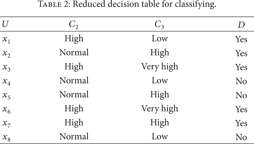
In the example shown in Table 1, the elementary sets defined by attributes C₂ and C₃ may be {x₁}, {x₂, x₃, x₆, x₇}, {x₄}, {x₅}, and {x₈}, while the subsets of the indiscernibility defined by C₁, C₂, and C₃ are similar to that defined by attributes C₂ and C₃. So it can be said that the attribute C₁ is superfluous and can be eliminated. A minimum set of condition attributes in which no superfluous attributes are included then can be obtained and used for diagnosis correctly, as shown in Table 2. The decision “machine malfunction”, however, is not dependent on the attributes C₂ and C₃ completely because the decision for class x₅ conflicts with class x₂. The condition attributes are the similar one by one in this case, so the decisions are not distinguished by the attributes. For these situations, the lower/upper approximation in rough sets theory can be employed to handle the conflictions. If we consider nondescript class, we will get the lower/upper approximation as shown in Tables 3 and 4, respectively.

Table 2:

Reduced decision table for classifying.

U	C 2	C 3	D
x 1	High	Low	Yes
x 2	Normal	High	Yes
x 3	High	Very high	Yes
x 4	Normal	Low	No
x 5	Normal	High	No
x 6	High	Very high	Yes
x 7	High	High	Yes
x 8	Normal	Low	No

Table 3:

Lower approximation.

U	C 2	C 3	D
x 1	High	Low	Yes
x3, x6	High	Very high	Yes
x4, x8	Normal	Low	No
x 7	High	High	Yes

Table 4:

Upper approximation.

U	C 2	C 3	D
x 1	High	Low	Yes
x 2	Normal	High	Yes
x3, x6	High	Very high	Yes
x4, x8	Normal	Low	No
x 5	Normal	High	No
x 7	High	High	Yes

The rules determined by the lower approximation of the decision are inevitably valid, while the rules from the upper approximation may be interpreted deterministically or nondeterministically. From the Table 3, the certain rules are as follows.

Rule 1. If vibration level is high, and the machine temperature is low, then the machine is in the condition of malfunction.

Rule 2. If vibration level is high, and the machine temperature is very high, then the machine is in the condition of malfunction.

Rule 3. If vibration level is normal, and the machine temperature is low, then the machine is not in the condition of malfunction.

Rule 4. If vibration level is high, and the machine temperature is high, then the machine is in the condition of malfunction.

And the probable rules obtained from Table 4 are as follows

Rule 1. If vibration level is high, and the machine temperature is low, then the machine is in the condition of malfunction.

Rule 2. If vibration level is normal, and the machine temperature is high, then the machine may be or may not be in the condition of malfunction.

Rule 3. If vibration level is high, and the machine temperature is very high, then the machine is in the condition of malfunction.

Rule 4. If vibration level is normal, and the machine temperature is low, then the machine is not in the condition of malfunction.

Rule 5. If vibration level is high, and the machine temperature is high, then the machine is in the condition of malfunction.

3. Case Study for Five-Plunger Pump Fault Diagnosis

The basic concept to apply the rough set theory to diagnose the pump faults is that the real information of characteristics for a verity of fault sorts serves as the condition attributes C, and the types of the fault module samples will be the decision attributes D in information system. We can set up the information table according to the real situation of the fault samples and then analyse the set of decision attributes, whether they are determined by the condition attributes, namely, whether there exists the dependence between C and D, shortly C ⇒ D. If the relation C ⇒ D exists it means that the decision set can be defined by category of condition attribute set. We can then calculate the condition set C whether the decision attributes are independent, remove a condition attribute according to whether it will damage the compatibility of the information table and abstract the diagnostic rules to diagnose the faults.

3.1. Construction of Condition Attributes for the Pump Fault Diagnosis

Vibration signals are extensively used in mechanical diagnostics. The reason for the wide use of vibration analysis may be due to the better understanding of vibration mechanism of machine operation and that the change in vibration signal can be easily attributed to the dynamic characteristics of the machine and its fault conditions. Of course, the five-plunger pumps generate vibration during their normal operation. Moreover, the vibration process is a good carrier of the pump and condition-related information, and we are measuring this as vibration signals and transforming it (by FFT operation), to obtain symptoms of condition.

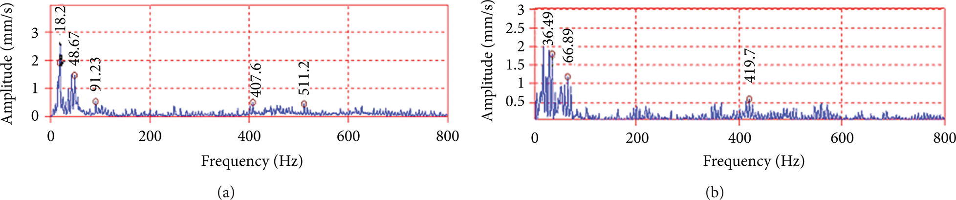
The testing work was carried out on an in-use pump in Tuha oil field in China. Under the consideration of the potential damage to the five-plunger pump and economic cost the faults were simulated mainly in the hydraulic-end of the pump during the experiment. Vibration signals were collected for both normal condition, and several different abnormal conditions. The accelerometers were mounted on the housing at the hydraulic-end of the pump. The crank shaft of the pump was running at approximately 370 rpm (6.17 Hz). The sampling rate was 2000 Hz. Figures 1 (a) and 1 (b) show the magnitude plot of the FFT of the vibration data (the frequency spectra of vibration signals).

Figure 1:

Frequency spectra from different vibration signals for different conditions. (a) Normal condition and (b) comprehensive faults both on the second and third inlet valves.

Figure 1 is an example of two typical frequency spectra derived from a dynamic vibration signal collected from the hydraulic-end. This figure shows a fault spectrum and a nonfault spectrum. It is clear that in this case (as well as many others) differences between spectra are quite straightforward. Designing automatic diagnostic tools for these cases is not a problem. Difficulties arise when the differences between signals (and spectra) representing different faults are much more subtle. Figure 2 is an example of two spectra representing well-developed faults of different nature that look similar. In this case, there is a considerable amount of uncertainties and a rigorous and finely tuned automatic diagnostic tool is required.

Figure 2:

Two frequency spectrum representing well-developed faults of different nature that looks similar. (a) and (b) Damage on the second plunger and forth exhaust valve, respectively.

Not only are individual samples of frequency spectra representing different faults often rather similar, but also the variability within a group of spectra that represent the same fault is often significant. Figures 3 (a) and 3 (b) show two frequency spectra that represent the same sample fault. The challenge is to provide early detection capability as well as distinction between fault types with a low risk of false alarms.

Figure 3:

Two frequency spectra that represent the same sample fault; (a) and (b) failure both on the second inlet valve.

In the fault diagnosis of the pump, the frequency spectra of the vibration signals contain complicated information of the running condition. To ensure the reliability of the rough set theory for the fault diagnosis of the pump, it is important to extract the condition attributes from the frequency spectra of the vibration signals.

The vibration energies of the horizontal direction in the hydraulic-end of the pump mainly concentrated on the 3 frequency bands: 0–60 Hz, 90–190 Hz, and 300–500 Hz. In the rest of the frequency range 500–800 Hz, there is little of energy distribution with almost no changes in level. The impulse amplitude modulation due to the load variation through the crank shaft revolution (6.17 Hz) is evident. As shown in the above figures, the range where the energy occupies in the frequency spectra is wide and the impulse peaks of frequency spectra are numerous and appear as clusters. These demonstrate the hydraulic pulsation caused by reciprocating motions of the plungers of the pump, the impact impulses excited by the open and shut-off of inlet and exhaust valves in the hydraulic-end of the pump, and the periodic impact vibration caused by the motions of the rotational and reciprocating parts. Due to the subtle changes of the fine frequency structure in vibration signal spectra, direct application of spectra would result in a difficult interpretation and the main events would be difficult to isolate. However, we know that, when the fault of the pump occurs, the changes of the vibration of excitation resource not only lead to changes in each class fault pattern but also result in changes in the overall energy content of the signal which will lead to an increase or decrease in the general spectrum level. So we can utilize these changes to extract features of the frequency components from the spectra and then employ the fuzzy diagnostic method to identify the conditions of the pump. The values of the constituent parts of the frequency band can represent the energy level of the vibration signal in the frequency domain.

Eight features are selected from the frequency spectra obtained from the vibration signals tested on the horizontal direction of the hydraulic-end of the pump. These features are defined as follows.

1. f₁: 5 kHz peak energy, to perform the peak energy analysis of the vibration signal, a three-step method is proposed, consisting of (a) using a band-pass filter of high cut-off frequency, for example, 5 kHz, to extract the lower and higher components from the acquired signal in time domain by removing the other events, (b) demodulating the reserved time signal, (c) transforming the demodulated signal to the frequency domain obtaining the 5 kHz spectrum, and then selecting the highest magnitude as the 5 kHz peak energy.

2. f₂: 5 kHz total peak energy.

3. f₃: the peak magnitude in the frequency range of 0–36 Hz which is mainly excited by the unbalance reciprocating motions of the plungers. The revolution of the crank shaft is 317 rpm (6.17 Hz), so the frequency of the plunger motion is about 31 Hz (5 × 6.17).

4. f₄: the peak magnitude in frequency range of 37–66 Hz. This frequency range represents the vibration frequency of the open and setting-down of inlet and exhaust valves and the changes of the direction of the impulse forces applied by the changes of the motions of the plungers.

5. f₅: the peak magnitude in range of low-middle frequency section of 67–100 Hz.

6. f₆: the peak magnitude in range of middle frequency section of 101–250 Hz.

7. f₇: the peak magnitude in range of middle-high frequency section of 251–500 Hz.

8. f₈: the peak magnitude in range of high frequency section of 501–800 Hz.

The features 5 to 8 are all of the harmonics of the frequency components of motions of the crank and plungers. These eight eigenvalues compose the crisp universal set F = {f₁, f₂, f₃, f₄, f₅, f₆, f₇, f₈} of the condition features. Table 5 shows the eight eigenvalues for normal running condition and different types of faults simulated in the hydraulic end of the pump. Four major types of mechanical faults, namely, failure on the second inlet valve, failure on the second plunger assembly, damage on the forth exhaust valve, and comprehensive faults both on the second and third inlet valves, are considered here. Among them, failure on plunger assembly is the most common fault that contributes nearly 56% of the pump faults. Inlet valve and exhaust valve are easily damaged components which account for about 11% and 13% of the pump faults, respectively. There are 14 sample sets representing 5 different types of the conditions given in Table 5. These 5 different types of conditions denote the decision set of fault causes D = {d _i } (i = 1, 2, 3, 4, 5). The decision attributes can be described as

$D=\{\begin{array}{cc}{d}_{\mathrm{1}}=\mathrm{1}\hfill & \text{Normal}\hfill \\ d_{\mathrm{2}}=\mathrm{2}\hfill & \mathrm{2}\text{nd}\mathrm{\hspace{0.17em}\hspace{0.17em}}\text{inlet}\hfill \\ d_{\mathrm{3}}=\mathrm{3}\hfill & \mathrm{2}\text{nd}\mathrm{\hspace{0.17em}\hspace{0.17em}}\text{plunger}\hfill \\ d_{\mathrm{4}}=\mathrm{4}\hfill & \mathrm{4}\text{th}\mathrm{\hspace{0.17em}\hspace{0.17em}}\text{exhaust}\hfill \\ d_{\mathrm{5}}=\mathrm{5}\hfill & \mathrm{2}\text{nd}\mathrm{\hspace{0.17em}\hspace{0.17em}}\mathrm{3}\mathrm{rd}\mathrm{\hspace{0.17em}\hspace{0.17em}}\text{inlet}.\hfill \end{array}$

(3)

Table 5:

Simulated data of the different fault conditions of a five-plunger pump.

Samples	Condition features								Technical states
	f 1	f 2	f 3	f 4	f 5	f 6	f 7	f 8
x 1	0.1449	0.3789	0.7	1.22	0.53	1.07	0.9	0.12	Normal
x 2	0.1078	0.237	0.8	1.3	0.5	1.2	0.9	0.15	Normal
x 3	0.0818	0.1932	0.85	1.6	0.45	0.87	0.72	0.15	2nd inlet
x 4	0.0779	0.1903	0.8	1.7	0.5	0.85	0.85	0.15	2nd inlet
x 5	0.0856	0.196	0.9	1.5	0.4	0.9	0.6	0.15	2nd inlet
x 6	0.2035	0.5404	0.5	1.25	0.45	1.55	1.2	0.24	2nd plunger
x 7	0.2003	0.5418	0.4	1.4	0.5	1.6	1.0	0.18	2nd plunger
x 8	0.2066	0.539	0.6	1.1	0.4	1.5	1.4	0.3	2nd plunger
x 9	0.0778	0.1689	1.17	1.5	0.4	1.1	0.92	0.22	4th exhaust
x 10	0.0643	0.1406	1.3	1.3	0.4	1.1	1.0	0.25	4th exhaust
x 11	0.0912	0.1972	1.05	1.7	0.4	1.1	0.85	0.2	4th exhaust
x 12	0.234	0.58	0.54	1.67	0.3	1.8	1.25	0.27	2nd 3rd inlet
x 13	0.244	0.5503	0.55	1.75	0.4	1.8	1.0	0.2	2nd 3rd inlet
x 14	0.224	0.5503	0.55	1.6	0.2	1.8	1.5	0.35	2nd 3rd inlet

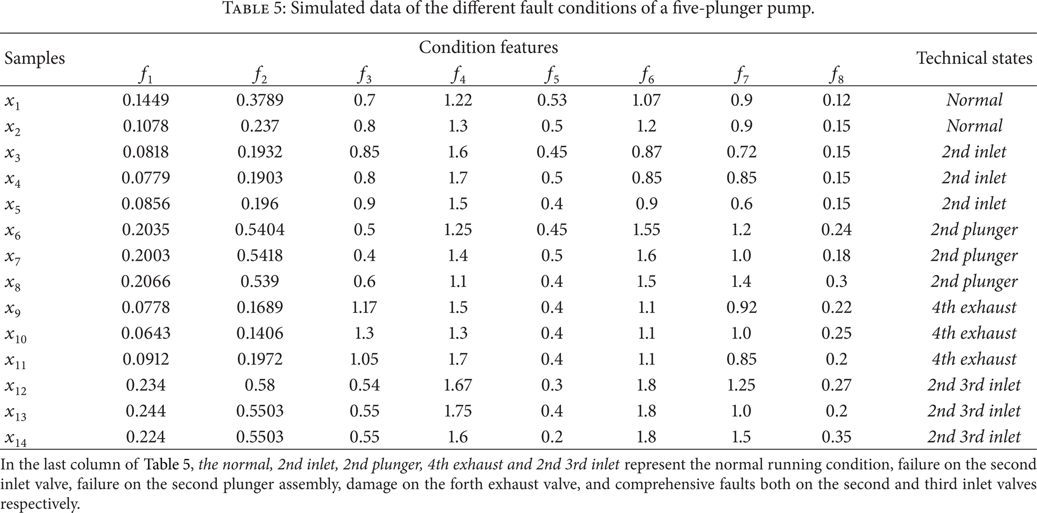
In the last column of Table 5, the normal, 2nd inlet, 2nd plunger, 4th exhaust and 2nd 3rd inlet represent the normal running condition, failureon the second inlet valve, failureon the second plunger assembly, damage on the forth exhaust valve, and comprehensive faults both on the second and third inlet valves respectively.

3.2. Discretization of Continuous-Valued Attributes for the Pump Fault Diagnosis

It can be seen from Table 5 that the condition attributes are continuous variables. They take on numerical values and have a linearly ordered range of values. When dealing with the data of the attributes in the pump diagnosis in the context of rough sets methodology, only the discrete-valued attributes can be used to select the group of condition attributes [15, 16]. So the range of a continuous-valued attribute should be partitioned into subranges. Such a process is known as discretization. However, discretization should be done in such a way to provide useful classification information with respect to the classes within an attribute's range. That is, the purpose of the discretization of continuous-valued attributes is to translate the continuous values into some qualitative characters which are compatible with the information table. This translation involves a division of the original domain into some subintervals and an assignment of qualitative codes to these subintervals. Definition of boundary values of the subintervals can influence considerably the quality of the classifications. Basically, a threshold value, T _i (i = 1, 2, …, N, N is the maximum group number of the condition attributes), for a continuous-valued attribute, c _i , is first determined. The set c _i < T _i (the value of attribute c _i which is less than T _i ) is assigned to a certain code, while c _i ≥ T _i (the value of attribute c _i that is greater than or equal to T _i ) is assigned to the other code. Such a threshold value, T _i , is called a quantization parameter. More specifically, given an information system, S, which is composed of M training examples, the discretization of a continuous-valued attribute, c _i , can be based on maximum covariance between the classes for the selection of a quantization parameter, to partition the domain range of c _i into two subdomains. Using a criterion of the consistency of classification it is possible to judge the consistence between the information systems before and after discretization. The details of the algorithm are as follows.

1. Initiate the number of classes, m = 2.

2. Set the initial number of condition attribute, n = 1.

3. Sort the training samples according to the condition attribute values of nth dimension from the smallest to the largest.

4. Classify the condition attributes sorted of the nth dimension.

5. Take boundary value of the condition attributes of adjacent two classes as the quantization parameter. Thus, for each continuous-valued attribute, M-1 evaluations will take place. (Analysis shows that the potential quantization parameter for partitioning the continuous-valued attribute will not lie between a pair of training samples with the same class in the sorted sequence. In other words, the best quantization parameter always lies between a pair of training samples belonging to different classes in the sorted sequence. This means that the evaluation of a potential quantization parameter will only be carried out when a pair of training samples with different classes is spotted.)

6. Quantitate the continuous-valued condition attributes using the quantization parameter of these two condition attributes and then calculate the covariance, σ_{m, n}, between them for mth class.

7. Partition the set of training samples into two subsets at each candidate quantization parameter; compute the consistency of classification of the resulting partition. The consistency, denoted by Q _U (X), can be formalized as follows:

   $Q_U\left(X\right)=\frac{{\sum }_{X∊\left(U/C\right)}\eta (R_{*}\left(X\right))}{\eta \left(U\right)},$

   (4)

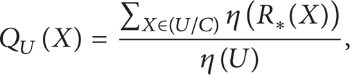
   where R_*(X), the lower approximation of X, is the set of all elements of U which can be certainly classified as elements of X using the set of attributes C · η(R_*(X)) and η(U) denote the cardinality of the sets R_*(X) and U, respectively. The criterion of the consistency of classification (4) gives the ratio of all correctly classified objects to all objects in the system. At first, the consistency of classification for continuous-valued attributes should be computed. Then that of the discrete-valued attributes can be searched for, ensuring the same quality.

8. Let n = n + 1, then return to Step 3 until the final dimension condition attributes.

9. When m ≤ M₁, a given positive integer value, check whether the parameter table is comparative or not. If it is not compatible, let m = m + 1 and return to Step 2. When m > M₁, let m = m + 1, and return to Step 2, until m = M₂, maximum number of the technical classes, and M₁ < M₂.

10. According to the relationship of m and σ_{m, n}, σ_{m, n} will increase with m increasing for mth dimension condition attributes until m = m₀, then it will decrease with m still increasing. So the optimum classification number is at the turning point m₀ on the curve m-σ_{m, n}.

11. Again check whether the parameter table it is compatible or not. If it is not, then let m₀(n) = m₀(n) + 1, and return to Step 2, until it is compatible.

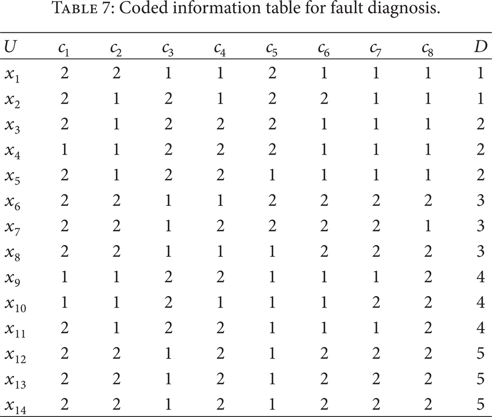
Let the condition symptoms be training samples, and let the eight features of the frequency spectrum, of the vibration signal be the condition attributes, that is f _i = c _i (i = 1, 2, …, 8), in fault models, respectively. The algorithm mentioned above is used first to determine the quantization parameters of each continuous-valued condition attributes presented in Table 5, with the optimum quantization parameters being shown in Table 6. Then the original values of the features can be translated into subintervals coded by numbers 1, 2,… with the determined quantization parameters. As a result of this translation the so-called coded information table, Table 7, is obtained which is further analysed. The rows in Table 5 describe the training samples of fault classes, and the columns represent the attributes of the samples. Tables 6 and 7 have the same format.

Table 6:

Quantization parameters of the continuous-valued condition attributes.

Condition attributes C	Condition features F	Quantization parameters/Codes
c 1	f 1	<0.08	1	≥0.08	2
c 2	f 2	<0.3	1	≥0.3	2
c 3	f 3	<0.8	1	≥0.8	2
c 4	f 4	<1.4	1	≥1.4	2
c 5	f 5	<0.45	1	≥0.45	2
c 6	f 6	<1.2	1	≥1.2	2
c 7	f 7	<1.0	1	≥1.0	2
c 8	f 8	<0.2	1	≥0.2	2

Table 7:

Coded information table for fault diagnosis.

U	c 1	c 2	c 3	c 4	c 5	c 6	c 7	c 8	D
x 1	2	2	1	1	2	1	1	1	1
x 2	2	1	2	1	2	2	1	1	1
x 3	2	1	2	2	2	1	1	1	2
x 4	1	1	2	2	2	1	1	1	2
x 5	2	1	2	2	1	1	1	1	2
x 6	2	2	1	1	2	2	2	2	3
x 7	2	2	1	2	2	2	2	1	3
x 8	2	2	1	1	1	2	2	2	3
x 9	1	1	2	2	1	1	1	2	4
x 10	1	1	2	1	1	1	2	2	4
x 11	2	1	2	2	1	1	1	2	4
x 12	2	2	1	2	1	2	2	2	5
x 13	2	2	1	2	1	2	2	2	5
x 14	2	2	1	2	1	2	2	2	5

3.3. Derivation of the Diagnosis Rules

In Table 7, there are 30 objects in the universe of discourse or condition discrimination domain U. This means that the information table for the fault diagnosis of the pump is composed of 30 implied diagnosis rules. These rules, however, are not completely meaningful in the practical diagnosis work. According to rough sets theory, the diagnosis rules can be directly extracted by calculating and reducing the data in the information table. Any set of limited decision, expressed by decision logical language (C ⇒ D), is called decision algorithm [15, 17, 18] or abbreviated as algorithm (C, D). All sets which cannot be omitted in the algorithm (C, D) compose the core of algorithm (C, D), expressed by core (C, D). The core values of the algorithm of the condition attributes in the information table can be computed by the following equation:

$\text{Core}\left(C,D\right)=\cap \text{Red}\left(C,D\right),$

(5)

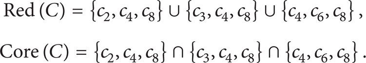
where Red (C, D) is all reduction family of the condition attributes. Through computation, it is found that the condition attributes c₁, c₂, c₃, c₅, c₆, and c₇ are redundant. This means that the information table will be compatible when removing the condition attributes c₁, c₂, c₃, c₅, c₆, and c₇, respectively, thus, the three reductions {c₂, c₄, c₈}, {c₃, c₄, c₈}, and {c₃, c₆, c₈} can be obtained and the core values are c₄ and c₈. That is

$\begin{array}{c}\text{Red}\left(C\right)=\left\{c_{\mathrm{2}},c_{\mathrm{4}},c_{\mathrm{8}}\right\}\cup \left\{c_{\mathrm{3}},c_{\mathrm{4}},c_{\mathrm{8}}\right\}\cup \left\{c_{\mathrm{4}},c_{\mathrm{6}},c_{\mathrm{8}}\right\},\\ \text{Core}\left(C\right)=\left\{c_{\mathrm{2}},c_{\mathrm{4}},c_{\mathrm{8}}\right\}\cap \left\{c_{\mathrm{3}},c_{\mathrm{4}},c_{\mathrm{8}}\right\}\cap \left\{c_{\mathrm{4}},c_{\mathrm{6}},c_{\mathrm{8}}\right\}.\end{array}$

(6)

The reduction {c₂, c₄, c₈} will be discussed in the following paragraph, while the meanings of the rest of the reductions are similar. After removing the superfluous condition attributes, the decision rule in the reduced information table can be deduced, that is, to compute the core of diagnosis rules C ⇒ D:

$\text{Core}\left(C⟹D\right)=\cap \text{Red}\left(C⟹D\right),$

(7)

where Red (C ⇒ D) is the set of all reduction C ⇒ D. The reduced diagnosis rules through the computation with (5) and (7) are shown in Table 8. The symbol (*) in Table 8 indicates that the influence of the values of the condition attributes on the fault diagnosis can be ignored.

Table 8:

Reduced information system for the pump fault diagnosis.

U	c 2	c 4	c 8	D
x1, x2	*	1	1	1
x3 ∼ x5	1	2	1	2
x6, x8	2	1	2	3
x 9	2	2	1	3
x10, x11	1	*	2	4
x12 ∼ x14	2	2	2	5

The fault diagnosis rules in Table 8 can be expressed with decision logical language.

Rule 1. (c₂ = 1) and (c₈ = 1) ⇒ D = d₁ = 1.

Rule 2. (c₂ = 1) and (c₄ = 2) and (c₈ = 1) ⇒ D = d₂ = 2.

Rule 3. (c₂ = 2) and (c₄ = 1) and (c₈ = 2) ⇒ D = d₃ = 3.

Rule 4. (c₂ = 2) and (c₄ = 2) and (c₈ = 1) ⇒ D = d₃ = 3.

Rule 5. (c₂ = 1) and (c₈ = 2) ⇒ D = d₄ = 4.

Rule 6. (c₂ = 2) and (c₄ = 2) and (c₈ = 2) ⇒ D = d₅ = 5.

The above rules can be translated into the logical statements (if…then…). For example, the meaning of the rule, (c₂ = 1) and (c₄ = 2) and (c₈ = 1) ⇒ D = d₂ = 2, is as follows.

• If 5 kHz peak energy (c₂) is less than 0.3 and the peak magnitude in frequency range of 37–66 Hz (c₄) is equal to or larger than 1.4 and the peak magnitude in range of high frequency section of 501–800 Hz (c₈) is less than 0.2, then the fault of the pump takes place likely on the second inlet valve.

Similar analysis can be carried out to derive reasonable rules for fault diagnosis when a pump has been detected. This shows that the proposed approach is able to gather a set of rules, which describes the general pattern of decision making by domain experts. With the rules extracted, a knowledge-based system can be developed to diagnose the pump faults.

3.4. Test Result Analysis

With the rules described above, the technical states of the pump can be diagnosed. Some of the test samples corresponding to normal running and with various fault conditions of the pump are shown in Table 9. Based on the sample data of the pump under different conditions, the coded condition attributes in the form of an information table (Table 10) are established by the discretization algorithm discussed in Section 3.2. The reduction and the core of the pump with different running conditions are then determined. This result in a minimum attribute set for diagnosing the pump faults. Both the minimum coded condition attributes and one decision attribute (D) are depicted in Table 11. Based on the rules extracted, the final diagnosis results of the detected pump can be discussed as follows.

Table 9:

Samples diagnosed of the pump.

Samples	f 1	f 2	f 3	f 4	f 5	f 6	f 7	f 8	Fault types
y 1	0.1189	0.2896	0.75	1.38	0.54	1.16	0.71	0.14	Normal
y 2	0.0802	0.2292	0.83	1.74	0.47	0.86	0.97	0.11	2nd inlet
y 3	0.2438	0.6403	0.44	1.35	0.54	1.77	1.12	0.25	2nd plunger
y 4	0.0837	0.1604	1.24	1.64	0.32	1.47	0.97	0.27	4th exhaust
y 5	0.288	0.5009	0.62	1.66	0.28	1.94	1.3	0.31	2nd 3rd inlet
y 6	0.2354	0.5697	0.6	1.58	0.3	1.9	1.4	0.33	2nd 3rd inlet
y 7	0.2601	0.7211	0.73	1.37	0.6	1.81	0.8	0.31	2nd plunger
y 8	0.2106	0.5785	0.55	1.24	0.4	1.7	1.2	0.26	2nd plunger
y 9	0.0755	0.1845	0.8	1.65	0.5	0.91	0.7	0.13	2nd inlet
y 10	0.0782	0.1771	1.05	1.9	0.45	1.25	0.84	0.25	4th exhaust
y 11	0.0775	0.1784	1.06	2.1	0.35	1.08	0.6	0.24	4th exhaust

Table 10:

Discretization attributes of the samples in Table 9.

Samples	c 1	c 2	c 3	c 4	c 5	c 6	c 7	c 8
y 1	2	1	1	1	2	1	1	1
y 2	2	1	2	2	2	1	1	1
y 3	2	2	1	1	2	2	2	2
y 4	2	1	2	2	1	2	1	2
y 5	2	2	1	2	1	2	2	2
y 6	2	2	1	2	1	2	2	2
y 7	2	2	1	1	2	2	1	1
y 8	2	2	1	1	1	2	2	2
y 9	1	1	2	2	2	1	1	1
y 10	1	1	2	2	2	2	1	2
y 11	1	1	2	2	1	1	1	2

Table 11:

Diagnosis results for different fault types.

Samples	c 2	c 4	c 8	D	Diagnostic results
y 1	*	1	1	d1 = 1	Normal
y 2	1	2	1	d2 = 1	2nd inlet
y 3	2	1	2	d3 = 3	2nd plunger
y 4	1	*	2	d4 = 4	4th exhaust
y 5	2	2	2	d5 = 5	2nd 3rd inlet
y 6	2	2	2	d5 = 5	2nd 3rd inlet
y 7	2	1	2	d3 = 3	2nd plunger
y 8	2	1	2	d3 = 3	2nd plunger
y 9	1	2	1	d2 = 2	2nd inlet
y 10	1	*	2	d4 = 4	4th exhaust
y 11	1	*	2	d4 = 4	4th exhaust

Rule 1. Because the peak magnitudes in frequency range of 37–66 Hz (f₄ = 1.38) are less than 1.4 (c₄ = 2) and the peak magnitude in range of high frequency section of 501–800 Hz (f₈ = 0.14) of sample y₁ is less than 0.2 (c₈ = 1), the sample y₁ represents the pump in normal condition (d₁ = 1).

Rule 2. Because 5 kHz peak energies (f₂ = 0.2292 and f₂ = 0.1845) are less than 0.3 (c₂ = 1), the peak magnitudes in frequency range of 37–66 Hz (f₄ = 1.74 and f₄ = 1.65) are larger than 1.4 (c₄ = 2), and the peak magnitudes in range of high frequency section of 501–800 Hz (f₈ = 0.11 and f₈ = 0.13) are less than 0.2 (c₈ = 1) of samples y₂ and y₉, the samples y₂ and y₉ are detected as the fault of the pump takes place likely on the second inlet valve (d₂ = 2).

Rule 3. Because 5 kHz peak energies (f₂ = 0.6403, f₂ = 0.7211, and f₂ = 0.5785) are larger than 0.3 (c₂ = 2), the peak magnitudes in frequency range of 37–66 Hz (f₄ = 1.35, f₄ = 1.37, and f₄ = 1.24) are less than 1.4 (c₄ = 1), and the peak magnitudes in range of high frequency section of 501–800 Hz (f₈ = 0.25, f₈ = 0.31, and f₈ = 0.26) of samples y₃, y₇ and y₈ are larger than 0.2 (c₈ = 2), the samples y₃, y₇, and y₈ can be diagnosed as the fault on the second plunger assembly of the pump (d₃ = 3).

Rule 5. Because 5 kHz peak energies (f₂ = 0.1604, f₂ = 0.1771 and f₂ = 0.1784) are less than 0.3 (c₂ = 1) and the peak magnitudes in range of high frequency section of 501–800 Hz (f₈ = 0.27, f₈ = 0.25, and f₈ = 0.24) of samples y₄, y₁₀ and y₁₁ are larger than 0.2 (c₈ = 2), the samples y₄, y₁₀, and y₁₁ indicate that the pump runs under abnormal condition withfault on the forth exhaust valve (d₄ = 4).

Rule 6. Because 5 kHz peak energies (f₂ = 0.5009 and f₂ = 0.5697) are larger than 0.3 (c₂ = 2), the peak magnitudes in frequency range of 37–66 Hz (f₄ = 1.66 and f₄ = 1.58) are larger than 1.4 (c₄ = 2), and the peak magnitudes in range of high frequency section of 501–800 Hz (f₈ = 0.31 and f₈ = 0.33) of samples y₅ and y₆ are larger than 0.2 (c₈ = 2), the samples y₅ and y₆ show that the faults of the pump take place likely on the second and third inlet valves at the same time (d₅ = 5).

According to the rules, we can reach all the diagnosis results. It can be seen from Table 11 that the decision results of the samples diagnosed are identical to the experiment results (Table 9). Generally, the diagnostic results are quite right. We would like to point out that the samples used here are not sufficient but are practically enough to illustrate the strategy with rough sets theory and how the original data set is transformed into a diagnostic information system directly.

4. Conclusion

This work shows that the basic concepts of rough sets theory provide a way to recognize and diagnose the pump faults. A practical case is used to illustrate the effectiveness of the technique. It is found that the preferential information about certain condition of the pump can be obtained easily and an adapted information table can be constructed readily by using the rough set approach. With the adapted information table established, the minimal diagnostic rule set that exits in a training data set can be obtained to classify technical states of the considered object. This rough approach makes a maintenance engineer in an oil field able to carry out fault diagnosis in an efficient manner and to know what kind of fault information is unimportant or redundant, which will not influence the fault diagnosis result, being missed or mistake occurred. The diagnostic investigation is done on data froma five-plunger pumpin outdoor conditions on a real industrial object. Results show that the new approach can effectively identify different operating states of the pump, which will supply as a basis for the detection and diagnosis of the pump faults.