Sage Journals: Discover world-class research

Abstract

Size optimization of double-layer scallop domes subjected to static loading is focused in the present paper. As this type of space structures possesses a large number of the structural elements, optimum design of such structures results in efficient structural configurations. In this paper, optimization task is achieved using firefly algorithm (FA) by taking into account linear and nonlinear responses of the structure. In the nonlinear optimization process only the geometrical nonlinearity effects are included. The numerical results demonstrate that nonlinear optimization provides more efficient structures compared with the linear one.

1. Introduction

As the space structures are employed to cover wide span column-free areas, they have a huge number of structural elements, and, therefore, sufficient attention must be paid to systematic designing of these structures. For this purpose, design of space structures can be conveniently achieved by employing optimization techniques. It is obvious that an optimal design has a great influence on the economy and safety of all types of the structures. In this case, optimizing space structures results in more efficient structural configurations. The present study is devoted to design optimization of a specific type of space structures denoted as scallop domes [1]. Configuration of scallop domes includes alternate ridged and grooves that radiate from the centre. There are many actual examples of scallop domes that are constructed throughout the world.

In the recent years, much progress has been made in optimum design of space structures by considering linear behavior [2 –4]. It is observed that some trusses show nonlinear behavior even in usual range of loading [5, 6]. Therefore, neglecting nonlinear effects in design optimization of these structures may lead to uneconomic designs.

In this study, double-layer scallop domes are designed for optimal weight considering linear and nonlinear behaviors. In the case of nonlinear optimization geometrical nonlinearity effects are taken into account. All of the structural optimization problems have two main phases: analysis and optimization. In the analysis phase, ANSYS [7] is employed and in the optimization phase, firefly algorithm (FA) [8] as an element of artificial intelligence (AI) is utilized. In the field of civil and structural engineering many applications of AI have been reported in the literature [9 –15]. The FA is coded in MATLAB [16]. In this paper, the design variables are cross-sectional areas of the structural elements. The design constraints involved here are nodal displacements and element stresses constraints. Three illustrative examples are presented and the numerical results reveal that the nonlinear optimization of scallop domes results in efficient structural configuration compared with the linear optimization process.

2. Scallop Domes

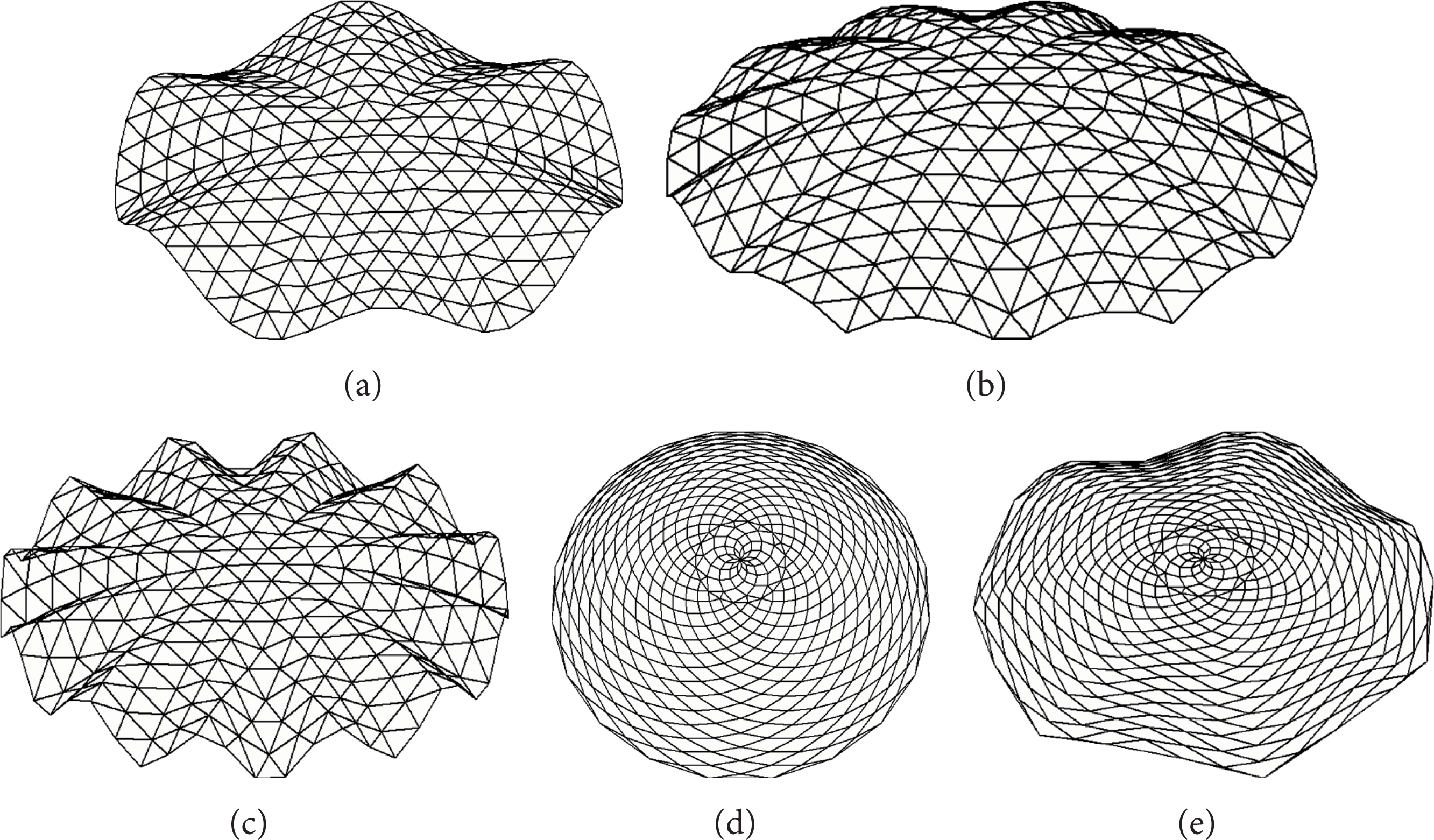
The dome shown in Figure 1(a) illustrates a perspective view of a [diamatic] dome. The plan of this dome has been shown in Figure 1(b). As shown in Figure 1(c), the border members of this dome are situated along meridional ribs and circumferential rings. Meridional ribs and circumferential rings on a spherical surface of Figure 1(c) correspond to the meridians and parallels on the surface of the earth.

Figure 1:

Example of scallop domes.

The perspective view of the dome configuration in Figure 1(d) is identical to the dome in Figure 1(a) in terms of the plan, the location of the meridional border members, and the height of the crown of the dome. However, as it is shown in Figure 1(d), the nodal points along every circumferential ring in the base diamatic dome are raised vertically such that the part of the ring between the borders is turned into an arch [1].

The dome that resulted from the arching of the members between the borders is called “scallop dome.” In fact, the arching of the nodes happens in such a way that firstly, the nodal points on the segmental borders remain in their original position (in particular, the position of the crown of the dome remains unchanged) and, secondly, the rise of the arches increases with distance from the crown of the dome. Of course, as it is also shown in Figure 1(e), the amount of rise increases closing to the middle of the segment.

The maximum rise for the circumferential ring, which occurs at the middle of each segment, is referred to as the “the amplitude of the ring.” The ring that is the furthest away from the crown, namely, the “base ring,” has the largest amplitude. This amplitude is referred to as “the amplitude of the dome” (Figure 1(d)). In this figure, the underneath curve shows the initial position of the base ring before the arching of the segments.

The amount of amplitude considering the architectural or structural requirements could be different. For example, the scallop dome in Figure 1(f) is similar to the scallop dome in Figure 1(d) except for its amplitude which is reduced into half.

In Figure 2, some domes are shown with gradual increase in amplitude.

Figure 2:

The variation of amplitude in scallop domes.

3. Arching Styles of Segments

The style of the variation of the height along with the circumferential ring can be accomplished in different ways. These height variations can be parabolic or sinusoidal. The scallop dome in Figure 3(a) is an example of parabolic variations [1].

Figure 3:

Arching styles of scallop domes.

The variation of height along the circumferential ring of the segment of the dome in Figure 1(d) is parabolic, whereas this variation of height in Figure 3(a) is sinusoidal.

The dome in Figure 3(c) like the one in Figure 3(b) includes 12 segments and the original domes of both are identical, but with different arching styles. Another example of sinusoidal scalloping is represented in Figure 3(e) which is obtained from scalloping the dome in Figure 3(c). Figure 4 clearly represents parabolic and sinusoidal arching. The horizontal base line in these figs is along with a circumferential ring between the border points, which may be assumed to be obtained by straightening out the ring between the border points along the ring illustrates parabolic and sinusoidal curves in Figure 4(a) and Figure 4(b), respectively.

Figure 4:

Parabolic and sinusoidal style of arching.

4. Theoretical Background of Nonlinear Analysis

In a linear static analysis it is assumed that the deflections and strains are very small and the stresses are smaller than the material yield stresses. Consequently, the stiffness can be considered to be independent of the displacements and forces and the finite element equilibrium equations are linear:

P = K δ,

(1)

where P, K, and δ are the external load vector, stiffness matrix, and nodal displacements vector, respectively.

This linearity implies that any increase or decrease in the load will produce proportional increase or decrease in displacements, strains, and stresses. But it is clear that, in many structures, at or near failure (ultimate) loads, the deflections and the stresses do not change proportionately with the loads. Either the stresses are so high that they no longer obey Hooke's law or else there are such large deflections that the compatibility equations cease to be linear. These two conditions are called material nonlinearity and geometric nonlinearity, respectively. In this study, a finite elements model based on geometrical analysis of scallop domes is performed by ANSYS. In the nonlinear structural analysis process, instead of the linear strain, a nonlinear strain [17] is used. Since the strains are nonlinear functions of the displacements the stress to strain relationship is nonlinear. In this case, the stiffness is dependent on the displacements and the strains. Obviously, the solution of the displacements cannot be obtained in a single step. Instead, the analysis is carried out by the incremental method combined with some iterative equilibrium corrections at every step [17]. In this work, the Newton-Raphson method of solution is used. The steps of the solution procedure are as follows.

Form tangent stiffness matrix (K_t) with the latest values of displacements and stresses:

K_{t} = \sum_{1}^{N_{e}} \int_{e} B^{T} D B d v,

(2)

where D is material stiffness matrix.

The incremental displacements equation is solved:

Δ δ = K_{t}^{- 1} Δ P + ψ,

(3)

where ΔP is part of the load vector to be applied at the current increment and ψ is the residual forces.

The incremental displacements are added to the total displacements:

δ \to δ + Δ δ .

(4)

The nonlinear strains are computed based on the latest estimate of the incremental strains Δ∊.

Total stresses are computed using the linear elastic stress strain relation:

σ \to σ + D Δ ∊ .

(5)

Contributions of the current Gauss point to the element internal forces are computed:

f_{i} = \int_{e} B^{T} σ d v .

(6)

Residual forces are computed:

ψ = \sum_{i = 1}^{n_{e}} (f_{i} - F),

(7)

where F contains the external forces and n_e is the number of elements.

Incremental loads are applied at the next increment and steps (1) to (7) are repeated until the process converges.

To increase the speed and accuracy of the nonlinear analysis, the applied loads are segmented into some loads termed substeps and then, in each substep, Newton-Raphson method is used.

5. Formulation of Optimization Problem

It is shown that consideration of nonlinear behavior in the optimum design of structures not only provides more realistic results, but also produces lighter structures [5, 6]. Nonlinear structural behavior arises from a number of causes, which can be grouped into geometrical and material nonlinearity. If a structure experiences large deformations, its changing geometric configuration can cause the structure to respond nonlinearly. Nonlinear stress-strain relationships are a common cause of material nonlinear behavior. One of the main factors that can influence a material's stress-strain properties is load history in elastoplastic response.

In optimal design problem of linear and nonlinear scallop domes, the aim is to minimize the weight of the structure under stress and displacement constraints. This optimization problem can be expressed as follows.

\begin{matrix} Minimize w (X) = \sum_{i = 1}^{n g} x_{i} \sum_{j = 1}^{n m} γ_{j} l_{j}, \\ subject to g_{d j} (X) = δ_{j} - δ_{j u} \leq 0, j = 1, \dots, p \\ g_{s k} (X) = σ_{k} - σ_{k u} \leq 0, k = 1, \dots, n e, \end{matrix}

(8)

where x_i, γ_j, and l_i are cross-sectional area of members belonging to group i, weight density, and length of jth element in this group, respectively; ng and nm are the total number of groups in the structure and the number of members in group n, respectively; δ_j and δ_ju are the displacement of jth joint and its upper bound, respectively; and p is the number of the nodes. Also σ_k and σ_ku are the stress of kth member and its upper bound, respectively; ne is the total number of members.

In the case of nonlinear optimization, design constraints include structural and stability constraints. The constraint ensuring the stability of the scallop dome during the optimization process is as follows:

g_{s} (X) = f_{a} - f_{u} \leq 0,

(9)

where f_a is applied load and f_u is ultimate load determined using nonlinear analysis.

The allowable tensile and compressive stresses, in the case of linear analysis, are used according to the AISC ASD (1989) code [18] as follows:

\begin{matrix} σ_{i a} = 0.6 F_{y} for tensile stress, \\ σ_{i a} = F_{c r} for compression stress, \end{matrix}

(10)

F_{c r} = {\begin{cases} \frac{[(1 - (λ_{i}^{2} / 2 C_{c}^{2})) F_{y}]}{[(5 / 3) + (3 λ_{i} / 8 C_{c}) - (λ_{i}^{3} / 8 C_{c}^{3})]} & λ_{i} < C_{c}, \\ \frac{12 π^{2} E}{23 λ_{i}^{2}} & λ_{i} \geq C_{c}, \end{cases}

(11)

where E is the modulus of elasticity, F_y is the yield stress of steel, C_c is the slenderness ratio (λ_i) dividing the elastic and inelastic buckling regions (C_c = √ 2π²E/F_y), λ_i is the slenderness ratio (λ_i = kl_i/r_i), k is the effective length factor, l_i is the member length and r_i is the radius of gyration.

In the case of nonlinear analysis, the critical stress for a tension member is simply taken as the yield stress of steel. For a compression member, the safety factors can be dropped from both the above mentioned expressions [5]:

F_{c r} = {\begin{cases} [(1 - \frac{λ_{i}^{2}}{2 C_{c}^{2}}) F_{y}] & λ_{i} < C_{c}, \\ \frac{π^{2} E}{λ_{i}^{2}} & λ_{i} \geq C_{c} . \end{cases}

(12)

In this study, penalty function method (PFM) is employed to handle the constraints of the structural optimization problem. PFM transforms the basic constrained optimization problem into alternative unconstrained one. The constrained optimization problem expressed by (8) can be converted into an unconstrained problem by constructing a function of the following form:

\begin{matrix} Φ (X, r_{p}) = f (X) + p (X), \\ p (X) = r_{p} \sum_{i = 1}^{n g} {[\max {0, g_{i} (X)}]}^{2}, \end{matrix}

(13)

where Φ, p, and r_p are the pseudoobjective function, penalty function, and positive penalty parameter, respectively.

6. Firefly Algorithm

In structural optimization problems, where the objective function and the constraints are highly nonlinear functions of the design variables, the computational effort spent in gradient calculations required by the mathematical programming algorithms is usually large. In recent years, it was found that probabilistic search algorithms are computationally efficient even if greater number of optimization cycles is needed to reach the optimum. Furthermore, probabilistic methodologies were found to be more robust in finding the global optima, due to their random search, whereas mathematical programming algorithms may be trapped into local optima. During the recent years, many advanced met-heuristic optimization algorithms have been proposed by researchers [19 –21]. However, in the present study, FA as a relatively new metaheuristic is used.

Gandomi et al. [22] employed FA for tackling benchmark complex optimization problems. Gholizadeh and Barati [23] compared the computational performance of particle swarm optimization (PSO), harmony search (HS), and FA algorithms for sizing and shaping optimisation of truss structures. Miguel et al. [24] employed FA for multimodal size, shape, and topology optimisation of truss structures.

The FA is a new metaheuristic optimization algorithm inspired by the flashing behavior of fireflies. FA is a population-based metaheuristic optimization algorithm. Fireflies communicate, search for prey, and find mates using bioluminescence with varied flashing patterns [22]. In order to develop the firefly algorithm, natural flashing characteristics of fireflies have been idealized using the following three rules [8].

All of the fireflies are unisex; therefore, one firefly will be attracted to other fireflies regardless of their sex.

Attractiveness of each firefly is proportional to its brightness; thus, for any two flashing fireflies, the less bright firefly will move towards the brighter one. The attractiveness is proportional to the brightness and they both decrease as their distance increases. If there is no brighter one than a particular firefly, it will move randomly.

The brightness of a firefly is determined according to the nature of the objective function.

The attractiveness of a firefly is determined by its brightness or light intensity which is obtained from the objective function of the optimization problem. However, the attractiveness β, which is related to the judgment of the beholder, varies with the distance between two fireflies. The attractiveness β can be defined by [22]

β = β_{0} e^{- γ \cdot r^{2}},

(14)

where r is the distance of two fireflies, β₀ is the attractiveness at r = 0, and γ is the light absorption coefficient.

The distance between two fireflies i and j at X_i and X_j, respectively, is determined using the following equation:

r_{i j} = ∥ X_{i} - X_{j} ∥ = \sqrt{\sum_{k = 1}^{d} {(x_{i, k} - x_{j, k})}^{2}},

(15)

where x_{i, k} is the kth parameter of the spatial coordinate x_i of the ith firefly.

In the FA, the movement of a firefly i towards a more attractive (brighter) firefly j is determined by the following equation:

X_{i} = X_{i} + β_{0} e^{- γ \cdot {r_{i j}}^{2}} (X_{j} - X_{i}) + α (rand - 0.5),

(16)

where the second term is related to the attraction, while the third term is randomization with α being the randomization parameter. Also, rand is a random number generator uniformly distributed in [0, 1].

In this paper, the modified equation proposed in [23] for computing α is employed as follows:

α = α_{\max} - \frac{α_{\max} - α_{\min}}{t_{\max}} \cdot t,

(17)

where α_max = 1 and α_min = 0.2. Also, t_max and t are the numbers of maximum iterations and present iteration, respectively.

7. Numerical Results

In the present work, three double-layer scallop domes with 6, 8, and 10 segments are considered. For all of the scallop domes, the span is 50.0 m, the height is 10 m, and the layer thickness is 1.5 m. The configurations of the mentioned scallop domes are shown in Figure 5. Young's modulus, mass density, and yield stress are 2.1 × 10¹⁰ kg/m², 7850 kg/m³, and 2.4 × 10⁶ kg/m², respectively. The computational time is measured in terms of CPU time of a PC Pentium IV 3000 MHz. A uniformly distributed load of 250 kg/m² is applied on the horizontal projection of the top layer.

Figure 5:

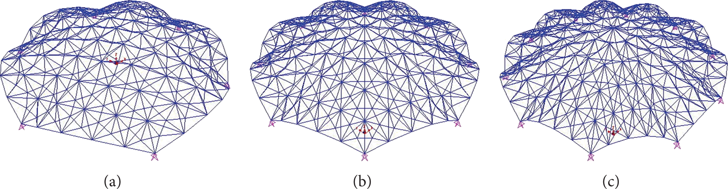
Double-layer scallop dome with (a) 6, (b) 8, and (c) 10 segments.

In the present study, the number of fireflies is 20 and the maximum number of iterations is 500.

The ratio between the number of structural analyses actually required in the optimization process and the maximum number of structural analyses that would have been performed if all iterations were completed in each optimization cycle can be computed as follows:

R = \frac{n p \times n g}{n p \times m n g},

(18)

where nf, ng, and mng are the number of fireflies, number of generations, and maximum number of generations, respectively.

The allowable vertical deflection is 10 cm and the stress constraints are given in (10) to (11). The discrete design variables are selected from a set of standard pipe profiles listed in Table 1. In this table, cross-sectional area and radius of gyration are given by A and r, respectively.

Table 1:

The available list of standard pipe profiles.

No.	Profile	A (cm²)	r (cm)

1	TUBO-D33.70×2.6	2.540	1.1000
2	TUBO-D48.30×2.6	3.730	1.6200
3	TUBO-D60.30×3.2	5.740	2.0200
4	TUBO-D76.10×3.2	7.329	2.5799
5	TUBO-D82.50×3.2	7.972	2.8060
6	TUBO-D88.90×3.2	8.616	3.0321
7	TUBO-D101.6×3.6	11.080	3.4672
8	TUBO-D108.0×3.6	11.810	3.6934
9	TUBO-D114.3×3.6	12.520	3.9161
10	TUBO-D127.0×4.0	15.450	4.3504
11	TUBO-D133.0×4.0	16.210	4.5629
12	TUBO-D139.7×4.0	17.050	4.8004
13	TUBO-D152.4×4.0	18.650	5.2483
14	TUBO-D159.0×4.0	19.480	5.4814
15	TUBO-D168.3×4.0	20.65	5.8102
16	TUBO-D193.7×4.5	26.75	6.6922
17	TUBO-D219.1×5.0	33.63	7.5716
18	TUBO-D244.5×5.4	40.56	8.4557
19	TUBO-D273.0×5.6	47.04	9.4570
20	TUBO-D298.5×5.9	54.23	10.3471
21	TUBO-D323.9×5.9	58.94	11.2450
22	TUBO-D355.6×6.3	69.13	12.3536
23	TUBO-D368.0×6.3	71.59	12.7895
24	TUBO-D406.4×6.3	79.19	14.1475
25	TUBO-D419.0×7.1	91.88	14.5645
26	TUBO-D457.2×7.1	100.4	15.9150

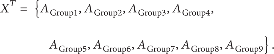
For all examples, the structural elements of each layer are divided into three groups and therefore the optimization problem includes nine design variables:

X^{T} = {A_{Group 1}, A_{Group 2}, A_{Group 3}, A_{Group 4}, A_{Group 5}, A_{Group 6}, A_{Group 7}, A_{Group 8}, A_{Group 9}} .

(19)

Example 1 (A 6-segment double layer scallop dome). The plane views of the 6-segment scallop dome together with its element groups are shown in Figure 6.

The optimization process considering linear and nonlinear behaviors is achieved and the results are given in Table 2.

In Table 3 the element stresses of the optimum design are compared with their corresponding allowable values and this comparison demonstrates that the solutions are feasible.

The nodal deflection of 6-segment optimum double-layer scallop dome found during the optimization process considering nonlinear behavior is represented in Figure 7.

Table 2:

Comparison of linear and nonlinear optimal designs for 6-segment double-layer scallop dome.

Design variables	Optimum design (cm²)
Design variables	Linear	Nonlinear

A _Group1	TUBO-D193.7×4.5	TUBO-D139.7×4.0
A _Group2	TUBO-D219.1×5.0	TUBO-D168.3×4.0
A _Group3	TUBO-D323.9×5.9	TUBO-D219.1×5.0
A _Group4	TUBO-D48.30×2.6	TUBO-D48.30×2.6
A _Group5	TUBO-D101.6×3.6	TUBO-D76.10×3.2
A _Group6	TUBO-D133.0×4.0	TUBO-D101.6×3.6
A _Group7	TUBO-D60.30×3.2	TUBO-D48.30×2.6
A _Group8	TUBO-D101.6×3.6	TUBO-D76.10×3.2
A _Group9	TUBO-D193.7×4.5	TUBO-D127.0×4.0

Weight (kg)	71994.14	44105.72
R	0.400	0.366
Overall time (min)	65.36	207.14
Maximum deflection (cm)	3.66	5.88

Table 3:

Comparison of element stresses in optimal designs for 6-segment double-layer scallop dome.

Group no.	Linear stresses (kg/cm²)				Nonlinear stresses (kg/cm²)
Group no.	σ⁻	σ_all⁻	σ⁺	σ_all⁺	σ⁻	σ_all⁻	σ⁺	σ_all⁺

1	−883.05	−1030.87	330.47	1440.00	−1353.55	−1483.97	538.04	2400.00
2	−1089.36	−1096.40	227.05	1440.00	−1745.17	−1774.71	367.48	2400.00
3	−1191.35	−1240.56	141.17	1440.00	−2022.98	−2031.79	218.55	2400.00
4	−274.93	−310.27	435.02	1440.00	−364.03	−594.68	548.77	2400.00
5	−668.37	−909.16	726.47	1440.00	−1027.25	−1177.98	1138.78	2400.00
6	−1091.87	−1122.73	623.65	1440.00	−1716.76	−1830.93	989.49	2400.00
7	−268.88	−485.61	132.90	1440.00	−457.95	−598.64	341.47	2400.00
8	−655.01	−893.69	122.29	1440.00	−1030.06	−1132.46	173.71	2400.00
9	−777.13	−1266.80	144.77	1440.00	−1411.50	−2080.07	309.72	2400.00

Figure 6:

The 6-segment scallop dome with its relative element groups.

Figure 7:

Deformed 6-segment nonlinear optimum double-layer scallop dome.

Example 2 (An 8-segment double-layer scallop dome). The plane views of the 8-segment scallop dome together with its element groups are shown in Figure 8.

The optimization process considering linear and nonlinear behaviors is achieved and the results are given in Table 4.

In Table 5 the element stresses of the optimum designs are compared with their corresponding allowable values and this comparison demonstrates that the solutions are feasible.

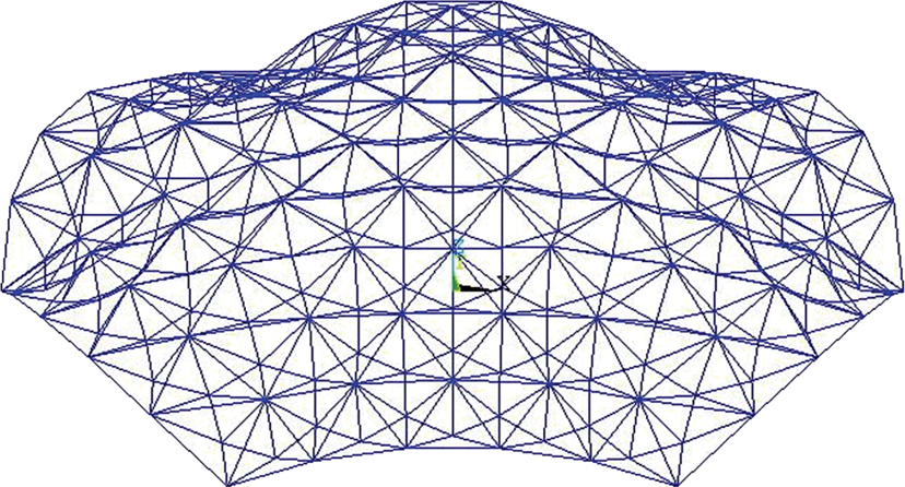
The nodal deflection of 8-segment optimum double-layer scallop dome found during the optimization process considering nonlinear behavior is represented in Figure 9.

Table 4:

Comparison of linear and nonlinear optimal designs for 8-segment double-layer scallop dome.

Design variables	Optimum design (cm²)
Design variables	Linear	Nonlinear

A _Group1	TUBO-D159.0×4.0	TUBO-D133.0×4.0
A _Group2	TUBO-D168.3×4.0	TUBO-D133.0×4.0
A _Group3	TUBO-D219.1×5.0	TUBO-D168.3×4.0
A _Group4	TUBO-D60.30×3.2	TUBO-D60.30×3.2
A _Group5	TUBO-D88.90×3.2	TUBO-D60.30×3.2
A _Group6	TUBO-D168.3×4.0	TUBO-D114.3×3.6
A _Group7	TUBO-D76.10×3.2	TUBO-D60.30×3.2
A _Group8	TUBO-D82.50×3.2	TUBO-D101.6×3.6
A _Group9	TUBO-D152.4×4.0	TUBO-D114.3×3.6

Weight (kg)	60602.13	42557.28
R	0.364	0.326
Overall time (min)	60.05	198.98
Maximum deflection (cm)	3.04	3.97

Table 5:

Comparison of element stresses in optimal designs for 8-segment double-layer scallop dome.

Group no.	Linear stresses (kg/cm²)				Nonlinear stresses (kg/cm²)
Group no.	σ⁻	σ_all⁻	σ⁺	σ_all⁺	σ⁻	σ_all⁻	σ⁺	σ_all⁺

1	−843.37	−894.52	403.45	1440.00	−1009.92	−1386.13	489.38	2400.00
2	−937.10	−938.83	104.20	1440.00	−1298.67	−1386.13	212.35	2400.00
3	−1071.14	−1096.40	99.74	1440.00	−1759.16	−1774.71	146.34	2400.00
4	−455.26	−601.24	404.45	1440.00	−389.68	−1152.38	437.70	2400.00
5	−546.85	−889.45	789.40	1440.00	−655.55	−898.26	1133.44	2400.00
6	−945.21	−1234.81	518.78	1440.00	−1580.30	−2016.69	856.67	2400.00
7	−672.56	−863.53	117.78	1440.00	−817.19	−1165.20	164.46	2400.00
8	−696.54	−720.95	246.91	1440.00	−612.11	−1732.07	74.48	2400.00
9	−834.87	−1230.00	504.21	1440.00	−1289.62	−2076.34	751.59	2400.00

Figure 8:

The 8-segment scallop dome with its relative element groups.

Figure 9:

Deformed 8-segment nonlinear optimum double-layer scallop dome.

Example 3 (A 10-segment double-layer scallop dome). The plane views of the 10-segment scallop dome together with its element groups are shown in Figure 10.

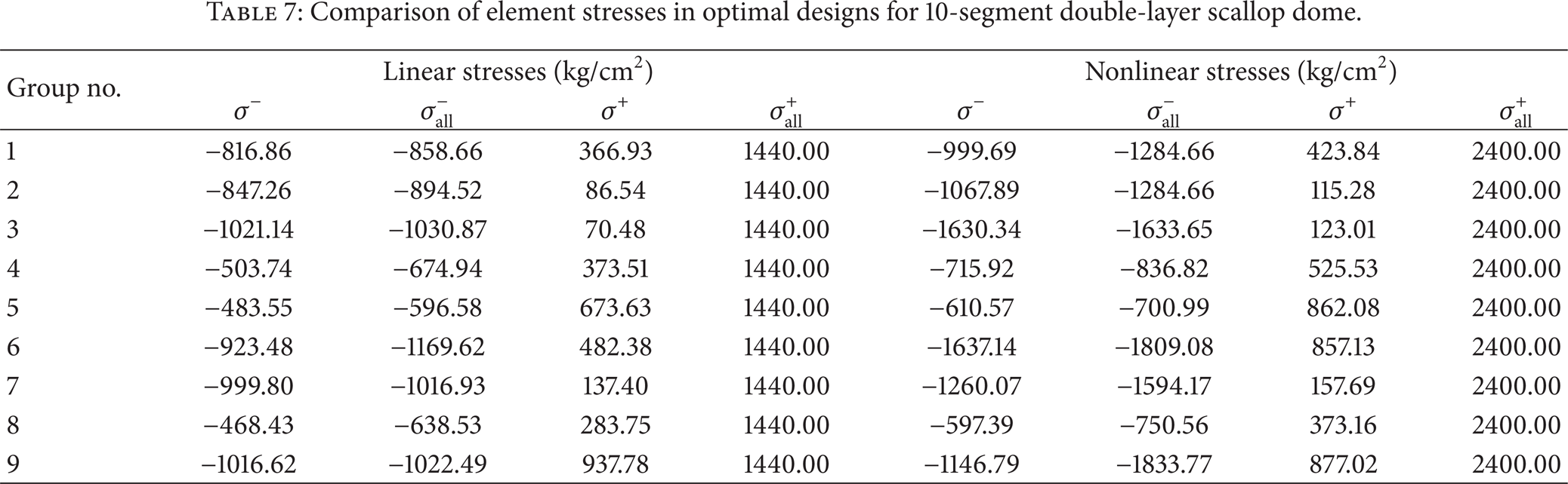
The optimization process considering linear and nonlinear behaviors is achieved and the results are given in Table 6. In Table 7 the element stresses of the optimum designs are compared with their corresponding allowable values and this comparison demonstrates that the solutions are feasible.

The nodal deflection of 10-segment optimum double-layer scallop dome found during the optimization process considering nonlinear behavior is represented in Figure 11.

Table 6:

Comparison of linear and nonlinear optimal designs for 10-segment double-layer scallop dome.

Design variables	Optimum design (cm²)
Design variables	Linear	Nonlinear

A _Group1	TUBO-D152.4×4.0	TUBO-D127.0×4.0
A _Group2	TUBO-D159.0×4.0	TUBO-D127.0×4.0
A _Group3	TUBO-D193.7×4.5	TUBO-D152.4×4.0
A _Group4	TUBO-D60.30×3.2	TUBO-D48.30×2.6
A _Group5	TUBO-D76.10×3.2	TUBO-D60.30×3.2
A _Group6	TUBO-D133.0×4.0	TUBO-D88.90×3.2
A _Group7	TUBO-D76.10×3.2	TUBO-D60.30×3.2
A _Group8	TUBO-D76.10×3.2	TUBO-D60.30×3.2
A _Group9	TUBO-D88.90×3.2	TUBO-D82.50×3.2

Weight (kg)	57185.91	41272.77
R	0.380	0.340
Overall time (min)	61.22	201.1
Maximum deflection (cm)	2.53	3.29

Table 7:

Comparison of element stresses in optimal designs for 10-segment double-layer scallop dome.

Group no.	Linear stresses (kg/cm²)				Nonlinear stresses (kg/cm²)
Group no.	σ⁻	σ_all⁻	σ⁺	σ_all⁺	σ⁻	σ_all⁻	σ⁺	σ_all⁺

1	−816.86	−858.66	366.93	1440.00	−999.69	−1284.66	423.84	2400.00
2	−847.26	−894.52	86.54	1440.00	−1067.89	−1284.66	115.28	2400.00
3	−1021.14	−1030.87	70.48	1440.00	−1630.34	−1633.65	123.01	2400.00
4	−503.74	−674.94	373.51	1440.00	−715.92	−836.82	525.53	2400.00
5	−483.55	−596.58	673.63	1440.00	−610.57	−700.99	862.08	2400.00
6	−923.48	−1169.62	482.38	1440.00	−1637.14	−1809.08	857.13	2400.00
7	−999.80	−1016.93	137.40	1440.00	−1260.07	−1594.17	157.69	2400.00
8	−468.43	−638.53	283.75	1440.00	−597.39	−750.56	373.16	2400.00
9	−1016.62	−1022.49	937.78	1440.00	−1146.79	−1833.77	877.02	2400.00

Figure 10:

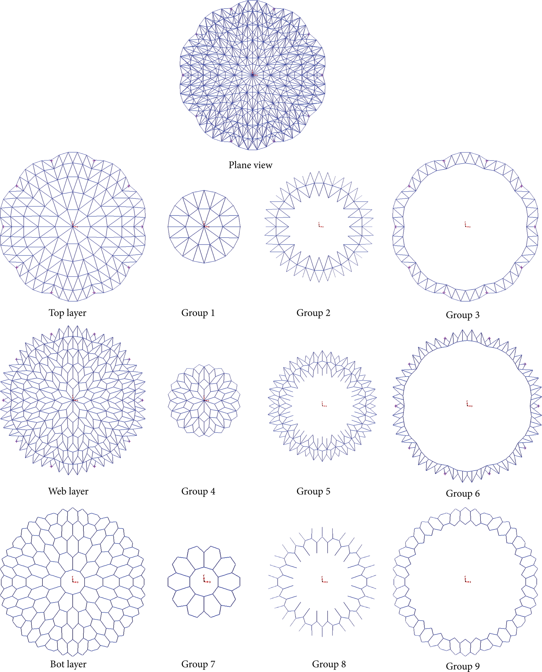
The 10-segment scallop dome with its relative element groups.

Figure 11:

Deformed 10-segment nonlinear optimum double-layer scallop dome.

8. Conclusions

The present study deals with size design optimization of scallop domes for static loading. The cross-sectional areas of the element groups are the design variables and the weight of the structure is the objective function of the optimization problem. The design variables are selected from a set of available standard sections; consequently, the optimization problem is discrete. Two optimization processes considering linear and nonlinear behavior of the structure are included. In the nonlinear optimization processes, geometrical nonlinearity is involved. In both optimization process, stress and deflection constraints are checked, but in the nonlinear optimization process the safety factors are dropped from the stress check equations. In order to implement the optimization, FA is employed. Considering 6-, 8-, and 10-segment scallop domes with nine element groups the optimization processes are achieved. In all examples the weight of nonlinear structure is significantly less than that of linear one. Also it is observed that in these examples, the number of required generations by the nonlinear optimization process is less than that of the linear one. The numerical results demonstrate that by taking into account the nonlinear behavior a significant reduction in the optimum weight of the scallop domes can be achieved compared with those of obtained involving linear behavior. Also, it is observed that by increasing the number of segments the weight of linear and nonlinear structures is decreased.

References

Nooshin

Tomatsuri

Fujimoto

, and Domes

, IASS97 Symposium on Shell & Spatial Structures: Design, Performance & Economics, CI-Premier Pte Ltd, Singapore, 1997.

Salajegheh

and Gholizadeh

, “Optimum design of structures by an improved genetic algorithm using neural networks,” Advances in Engineering Software, vol. 36, no. 11–12, pp. 757–767, 2005.

Kaveh

Farhmand Azar

, and Talatahari

, “Ant colony optimization for design of space trusses,” International Journal of Space Structures, vol. 23, no. 3, pp. 167–181, 2008.

Toğan

and Daloğlu

A. T.

, “Optimization of 3d trusses with adaptive approach in genetic algorithms,” Engineering Structures, vol. 28, no. 7, pp. 1019–1027, 2006.

Saka

M. P.

and Ulker

, “Optimum design of geometrically nonlinear space trusses,” Computers and Structures, vol. 41, no. 6, pp. 1387–1396, 1991.

Kamyab Moghdas

and Salajegheh

, “Size optimization of nonlinear scallop domes by an enhanced particle swarm algorithm,” International Journal of Civil Engineering, vol. 11, pp. 77–89, 2013.

ANSYS Release 10.0 Documentation, ANSYS, Inc., Houston, Tex, USA, 2006.

Yang

X. S.

, “Firefly algorithms for multimodal optimization,” in Stochastic Algorithms: Foundations and Applications, Watanabe

and Zeugmann

, Eds., vol. 5792 of Lecture Notes in Computer Science, pp. 169–178, Springer, Berlin, Germany, 2009.

Talatahari

, “Determining the optimum section of tunnels using ant colony optimization,” Mathematical Problems in Engineering, vol. 2013, Article ID 320360, 7 pages, 2013.

10.

Gholizadeh

Pirmoz

, and Attarnejad

, “Assessment of load carrying capacity of castellated steel beams by neural networks,” Journal of Constructional Steel Research, vol. 67, no. 5, pp. 770–779, 2011.

11.

Gandomi

A. H.

Talatahari

Yang

X. S.

, and Deb

, “Design optimization of truss structures using cuckoo search algorithm,” The Structural Design of Tall and Special Buildings, vol. 22, no. 17, pp. 1330–1349, 2013.

12.

Talatahari

Kheirollahi

Farahmandpour

, and Gandomi

A. H.

, “A multi-stage particle swarm for optimum design of truss structures,” Neural Computing and Applications, vol. 23, no. 5, pp. 1297–1309, 2013.

13.

Gholizadeh

and Samavati

O. A.

, “Structural optimization by wavelet transforms and neural networks,” Applied Mathematical Modelling, vol. 35, no. 2, pp. 915–929, 2011.

14.

Kamyab

and Salajegheh

, “Prediction of nonlinear time history deflection of scallop domes by neural networks,” International Journal of Optimization in Civil Engineering, vol. 1, pp. 419–432, 2011.

15.

Kamyab Moghadas

Keong

C. K.

, and Mohd

S. B.

, “Prediction of optimal design and deflection of space structures using neural networks,” Mathematical Problems in Engineering, vol. 2012, Article ID 712974, 18 pages, 2012.

16.

MATLAB—The Language of Technical Computing, The Math Works, Inc., Natick, Mass, USA, 2006.

17.

Crisfield

M. A.

, Non-Linear Finite Element Analysis of Solids and Structures, vol. 1, John Wiley & Sons, Chichester, UK, 1991.

18.

AISC, Manual of Steel Construction-Allowable Stress Design, American Institute of Steel Construction, Chicago, Ill, USA, 9th edition, 1989.

19.

Gholizadeh

, “Layout optimization of truss structures by hybridizing cellular automata and particle swarm optimization,” Computers and Structures, vol. 125, pp. 86–99, 2013.

20.

Gholizadeh

and Barzegar

, “Shape optimization of structures for frequency constraints by sequential harmony search algorithm,” Engineering Optimization, vol. 45, no. 6, pp. 627–646, 2013.

21.

Kaveh

and Talatahari

, “Particle swarm optimizer, ant colony strategy and harmony search scheme hybridized for optimization of truss structures,” Computers and Structures, vol. 87, no. 5–6, pp. 267–283, 2009.

22.

Gandomi

A. H.

Yang

X.-S.

, and Alavi

A. H.

, “Mixed variable structural optimization using Firefly Algorithm,” Computers and Structures, vol. 89, no. 23–24, pp. 2325–2336, 2011.

23.

Gholizadeh

and Barati

, “A comparative study of three metaheuristics for optimum design of trusses,” International Journal of Optimization in Civil Engineering, vol. 2, pp. 423–441, 2012.

24.

Miguel

L. F. F.

Lopez

R. H.

, and Miguel

L. F. F.

, “Multimodal size, shape, and topology optimisation of truss structures using the Firefly algorithm,” Advances in Engineering Software, vol. 56, pp. 23–37, 2013.

Optimum Design of Geometrically Nonlinear Double-Layer Domes by Firefly Metaheuristic Algorithm

Abstract

1. Introduction

2. Scallop Domes

3. Arching Styles of Segments

4. Theoretical Background of Nonlinear Analysis

5. Formulation of Optimization Problem

6. Firefly Algorithm

7. Numerical Results

8. Conclusions

References