Sage Journals: Discover world-class research

Abstract

Dynamic responses of a viscous fluid flow introduced under a time dependent pressure gradient in a rigid cylindrical tube subject to deformable porous surface layer have been investigated. The coupling effect of the fluid movement and the deformation of the porous medium in Laplace transform space have been studied. Governing equations are simplified for the solid displacement and the fluid velocity in the porous layer. Using Durbin's algorithm, in transformed domain analytic solutions are obtained, and time dependent variables are considered. Interaction between the solid and the fluid phases in the porous layer and its effects on fluid flow in tube are investigated under steady and unsteady flow conditions when the solid phase is either rigid or deformable. Significant effects of the porous surface layer on the flow in the tube have been observed.

1. Introduction

Richardson and Power [1] studied the deformation of a porous material with coupled fluid movements. Barry et al. [2] derived the analytic solutions for a shear fluid over a thin deformable porous layer on the walls of a two-dimensional channel considering the porosity and permeability of the porous layer as constants; therefore, the coupled equations are linear. Barry et al. [3] obtained a closed form solution for deformation of porous medium due to a source in a poroelastic medium. This solution shows an indication of the amount of swelling of the medium and subsequent deformation of the free surface as a function of the location of the point source and boundary condition. Presently, numerical simulation for viscous flow in the porous medium is more applicable. Pozrikidis [4], Wrobel [5], and Dwivedi et al. [6, 7] used the boundary element method in solving partial differential equations. However, there is still a lack of closed form analytic solution for shear flow over a deformable porous medium.

In this paper, the solutions in closed form for viscous fluid over a deformation porous layer in the cylinder are obtained in the Laplace transform space. The coupled equations for deformation and fluid velocity within the porous layer are shown in Figure 1. In the present work, the porous medium is isotropic and axially symmetric, and the deformation of solid is small. Assuming constant permeability of the porous medium, linear elasticity theory is applied to investigate the proposed problem. By Durbin's inversion method, the displacement of solid phase and the velocity of fluid are obtained in the time domain, and analytical solutions for three different situations of the porous layer (i.e., steady state deformation, rigid porous layer, and deformable porous layer) are obtained for a step or a sinusoid pressure gradient in an infinite tube.

Figure 1:

Schematic diagram shows the tube with a porous medium layer and the cylindrical coordinate.

2. Governing Equations

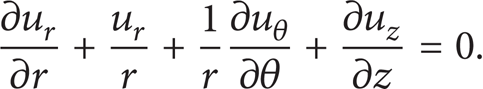
In cylindrical coordinate system as shown in Figure 1, the governing equations for the velocities of fluid phase, for zero convective, are given by

ρ_{f} (\frac{\partial υ_{r}}{\partial t} + υ_{r} \frac{\partial υ_{r}}{\partial r} + υ_{θ} \frac{\partial υ_{r}}{\partial θ} + υ_{z} \frac{\partial υ_{r}}{\partial z} - \frac{υ_{θ}^{2}}{r}) = - φ_{f} \frac{\partial p}{\partial r} + μ_{a} (\frac{\partial^{2} υ_{r}}{\partial r^{2}} + \frac{1}{r} \frac{\partial υ_{r}}{\partial r} + \frac{1}{r^{2}} \frac{\partial^{2} υ_{r}}{\partial θ^{2}} + \frac{\partial^{2} υ_{r}}{\partial z^{2}} - \frac{υ_{r}}{r^{2}} - \frac{2}{r^{2}} \frac{\partial υ_{θ}}{\partial θ}) + K (\frac{\partial u_{r}}{\partial t} - υ_{r}),

(1)

ρ_{f} (\frac{\partial υ_{θ}}{\partial t} + υ_{r} \frac{\partial υ_{θ}}{\partial r} + υ_{θ} \frac{\partial υ_{θ}}{\partial θ} + υ_{z} \frac{\partial υ_{θ}}{\partial z} + \frac{υ_{r} υ_{θ}}{r}) = - φ_{f} \frac{1}{r} \frac{\partial p}{\partial θ} + μ_{a} (\frac{\partial^{2} υ_{θ}}{\partial r^{2}} + \frac{1}{r} \frac{\partial υ_{θ}}{\partial r} + \frac{1}{r^{2}} \frac{\partial^{2} υ_{θ}}{\partial θ^{2}} + \frac{\partial^{2} υ_{θ}}{\partial z^{2}} - \frac{υ_{θ}}{r^{2}} + \frac{2}{r^{2}} \frac{\partial υ_{r}}{\partial θ}) + K (\frac{\partial u_{θ}}{\partial t} - υ_{θ}),

(2)

ρ_{f} (\frac{\partial υ_{z}}{\partial t} + υ_{r} \frac{\partial υ_{z}}{\partial r} + υ_{θ} \frac{\partial υ_{z}}{\partial θ} + υ_{z} \frac{\partial υ_{z}}{\partial z}) = - φ_{f} \frac{\partial p}{\partial z} + μ_{a} (\frac{\partial^{2}}{\partial r^{2}} + \frac{1}{r} \frac{\partial}{\partial r} + \frac{1}{r^{2}} \frac{\partial^{2}}{\partial θ^{2}} + \frac{\partial^{2}}{\partial z^{2}}) υ_{z} + K (\frac{\partial u_{z}}{\partial t} - υ_{z}) .

(3)

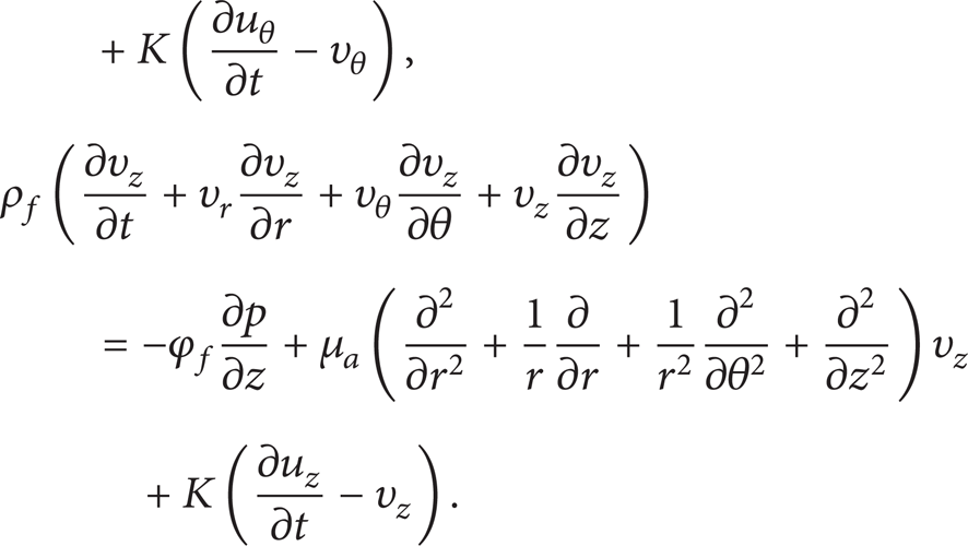
The equation of mass conservation of fluid becomes

\frac{\partial υ_{r}}{\partial r} + \frac{υ_{r}}{r} + \frac{1}{r} \frac{\partial υ_{θ}}{\partial θ} + \frac{\partial υ_{z}}{\partial z} = 0,

(4)

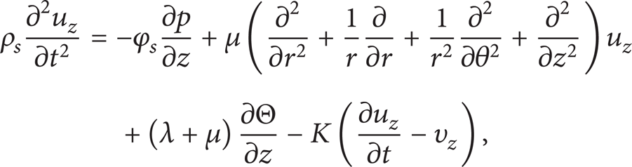
and equation for solid phase is

ρ_{s} \frac{\partial^{2} u_{r}}{\partial t^{2}} = - φ_{s} \frac{\partial p}{\partial r} + μ (\frac{\partial^{2}}{\partial r^{2}} + \frac{1}{r} \frac{\partial}{\partial r} + \frac{1}{r^{2}} \frac{\partial^{2}}{\partial θ^{2}} + \frac{\partial^{2}}{\partial z^{2}} - \frac{1}{r^{2}}) u_{r} - \frac{u_{r}}{r^{2}} - \frac{2}{r^{2}} \frac{\partial u_{θ}}{\partial θ} + (λ + μ) \frac{\partial Θ}{\partial θ} - K (\frac{\partial u_{r}}{\partial t} - υ_{r}),

(5)

ρ_{s} \frac{\partial^{2} u_{θ}}{\partial t^{2}} = - φ_{s} \frac{1}{r} \frac{\partial p}{\partial θ} + μ (\frac{\partial^{2}}{\partial r^{2}} + \frac{1}{r} \frac{\partial}{\partial r} + \frac{1}{r^{2}} \frac{\partial^{2}}{\partial θ^{2}} + \frac{\partial^{2}}{\partial z^{2}}) u_{θ} - \frac{u_{θ}}{r^{2}} + \frac{2}{r^{2}} \frac{\partial u_{θ}}{\partial θ} + (λ + μ) \frac{1}{r} \frac{\partial Θ}{\partial θ} - K (\frac{\partial u_{θ}}{\partial t} - υ_{θ}),

(6)

ρ_{s} \frac{\partial^{2} u_{z}}{\partial t^{2}} = - φ_{s} \frac{\partial p}{\partial z} + μ (\frac{\partial^{2}}{\partial r^{2}} + \frac{1}{r} \frac{\partial}{\partial r} + \frac{1}{r^{2}} \frac{\partial^{2}}{\partial θ^{2}} + \frac{\partial^{2}}{\partial z^{2}}) u_{z} + (λ + μ) \frac{\partial Θ}{\partial z} - K (\frac{\partial u_{z}}{\partial t} - υ_{z}),

(7)

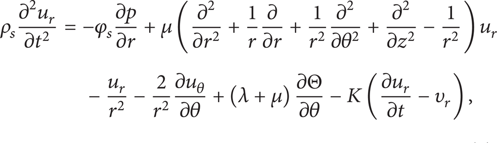
where the volume expansion is given by

Θ = \frac{\partial u_{r}}{\partial r} + \frac{u_{r}}{r} + \frac{1}{r} \frac{\partial u_{θ}}{\partial θ} + \frac{\partial u_{z}}{\partial z} .

(8)

In our case, an infinite long tube of radius a with a rigid wall, which consists a porous layer of thickness ∊_T and a fully developed flow as shown in Figure 1, is considered. The fluid is initially at rest and subjected to a time dependent pressure differential p = p₀(t) at the ends of the tube. Due to the assumption of an infinite tube, we assume that the pressure gradient is constant for each section of the tube; that is, $\partial p / \partial z = - G_{0} g (t)$ , where g(t) is nondimensional function of time and all variables are not z dependent. With the symmetry of the geometry of problem, there are no velocities along the radial and circumference directions; that is, υ_r = υ_θ = u_r = u_θ = 0 everywhere in the tube. When the flow and solid start impulsively from rest and without moving boundaries, under these conditions, that is, $\partial υ_{z} / \partial z = \partial υ_{z} / \partial θ = \partial u_{z} / \partial z = \partial u_{z} / \partial θ = 0$ and volume expression Θ = 0, (1), (2), and (4) are automatically satisfied.

By (3), we have

ρ_{f} (\frac{\partial υ_{z}}{\partial t}) = - φ_{f} \frac{\partial p}{\partial z} + μ_{a} (\frac{\partial^{2}}{\partial r^{2}} + \frac{1}{r} \frac{\partial}{\partial r}) υ_{z} + K (\frac{\partial u_{z}}{\partial t} - υ_{z}) .

(9)

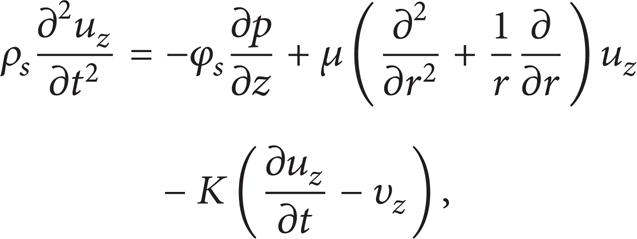
Also, (5) and (6) are automatically satisfied, and (7) for solid phase becomes

ρ_{s} \frac{\partial^{2} u_{z}}{\partial t^{2}} = - φ_{s} \frac{\partial p}{\partial z} + μ (\frac{\partial^{2}}{\partial r^{2}} + \frac{1}{r} \frac{\partial}{\partial r}) u_{z} - K (\frac{\partial u_{z}}{\partial t} - υ_{z}),

(10)

\frac{\partial u_{r}}{\partial r} + \frac{u_{r}}{r} + \frac{1}{r} \frac{\partial u_{θ}}{\partial θ} + \frac{\partial u_{z}}{\partial z} = 0 .

(11)

Taking Laplace transform of (9) and (10), we have

ρ_{f} s {\tilde{υ}}_{z} = - φ_{f} G_{0} + μ_{a} \nabla^{2} {\tilde{υ}}_{z} + K (s {\tilde{u}}_{z} - {\tilde{υ}}_{z}),

(12)

ρ_{s} s^{2} {\tilde{u}}_{z} = φ_{s} G_{0} + μ \nabla^{2} {\tilde{u}}_{z} + K (s {\tilde{u}}_{z} - {\tilde{υ}}_{z}),

(13)

where $\nabla^{2} = (\partial^{2} / \partial r^{2}) + (1 / r) (\partial / \partial r)$ .

Nondimensional variables are defined, for the convenience in the following analysis, as

\begin{matrix} \bar{r} = \frac{r}{a}, \bar{b} = \frac{b}{a}, {\bar{∊}}_{T} = \frac{∊_{T}}{a}, \bar{υ} = \frac{G_{0} \tilde{g} a^{2}}{μ_{a}} {\tilde{υ}}_{z}, \\ \bar{u} = \frac{G_{0} \tilde{g} a^{2}}{μ} {\tilde{u}}_{z}, \bar{q} = \frac{G_{0} \tilde{g} a^{2}}{μ_{f}} {\tilde{υ}}_{z}, \\ \bar{s} = \frac{ρ_{f} a^{2}}{μ_{f}} s = t_{0} s, \bar{t} = \frac{t}{t_{0}}, \end{matrix}

(14)

where t₀ = ρ_fa²/μ_f denotes the unit of time and followsnondimensional parameters arisen from the governing equations

γ = \frac{K μ_{f}}{μ ρ_{f}}, k^{2} = \frac{K a^{2}}{μ_{a}}, η = \frac{μ_{f}}{μ_{a}}, δ = \frac{ρ_{s}}{ρ_{f}} .

(15)

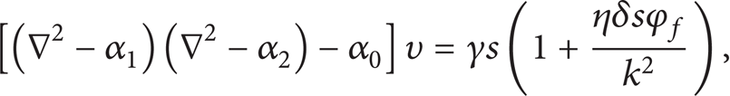
For convenience, the tilde (^∼) is dropped in the following analysis as all variables in the Laplace transform space are nondimensional hereafter. Substituting these expressions from (14) and (15) into (12) and (13), we obtain momentum (16) and (17), respectively. Consider

\nabla^{2} υ - (η s + k^{2}) υ + γ s u + φ_{f} = 0,

(16)

\nabla^{2} u - γ s (1 + \frac{η δ s}{k^{2}}) u + k^{2} υ + φ_{s} = 0 .

(17)

By taking φ_f = 1, K = 0, μ_a = μ_f, η = 1, and $\bar{υ} = \bar{q}$ and using (14) and (15) in (16), in the pure fluid phase outside of the porous medium, the governing equation of the pure fluid velocity is obtained in the following form:

(\nabla^{2} - s) q + 1 = 0 .

(18)

3. Analytical Solutions

3.1. Steady State Deformation

For steady state deformation of porous medium, the pressure gradient G(t) is applied steady, and all variables are time independent. Therefore, the governing equations can be represented, by letting s = 0 in (16), (17), and (18) as

\nabla^{2} υ - k^{2} υ + φ_{f} = 0,

(19)

\nabla^{2} u + k^{2} υ + φ_{s} = 0,

(20)

\nabla^{2} q + 1 = 0 .

(21)

In case of steady state deformation, at the interface between the porous layer and the pure fluid, the nondimensional boundary conditions and assumptions are as follows:

\begin{matrix} at r = 1 : υ = u = 0, \\ at r = 0 : \frac{\partial q}{\partial r} = 0, \\ at r = b = 1 - ∊_{T}, s = 0 : q = n φ_{f} υ, \\ \frac{\partial q}{\partial r} = \frac{1}{φ_{f}} \frac{\partial υ}{\partial r} = \frac{1}{φ_{s}} \frac{\partial u}{\partial r} . \end{matrix}

(22)

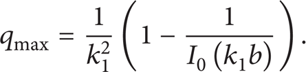
Therefore, the general solution of (21) can be obtained as

q = q_{0} + q_{1} \ln r - \frac{r^{2}}{4} .

(23)

When q₁ = 0, the maximum value of q reduces into q_max = q₀.

The general solutions of (19) and (20) can be obtained as

υ = A I_{0} (k r) + B K_{0} (k r) + \frac{φ_{f}}{k^{2}},

(24)

u = - [A I_{0} (k r) + B K_{0} (k r)] - \frac{r^{2}}{4} + u_{0} + u_{1} \ln r,

(25)

respectively, where I_n(z) and K_n(z) are the modified Bessel functions of the first and second kinds of order n.

Considering boundary conditions,

r = 1: υ = u = 0,

r = b = 1 – ∊_T, s = 0: q = nφ_fυ,

and solving (23), (24), and (25), we have

\begin{matrix} A = \frac{(φ_{f} / 2 k^{2}) (k (1 - ∊_{T}) K_{0} (k) + 2 K_{1} (k b))}{(K_{0} (k) I_{1} (k b) - K_{1} (k b) I_{0} (k))}, \\ B = \frac{(φ_{f} / 2 k^{2}) [k (1 - ∊_{T}) I_{0} (k) + 2 I_{1} (k b)]}{[K_{1} (k b) I_{0} (k) - K_{0} (k) I_{1} (k b)]}, \\ K_{0} (k) I_{1} (k b) - K_{1} (k b) I_{0} (k) \neq 0, \\ q_{\max} = q_{0} = \frac{{(1 - ∊_{T})}^{2}}{4} + \frac{η φ_{f}^{2}}{2 k^{2} [K_{0} (k) I_{1} (k b) - K_{1} (k b) I_{0} (k)]} \times [k (1 - ∊_{T}) (K_{0} (k) I_{0} (k b) - I_{0} (k) K_{0} (k b)) + 2 (K_{1} (k b) I_{0} (k b) - I_{1} (k b) K_{0} (k b))] + \frac{η φ_{f}^{2}}{k^{2}} . \end{matrix}

(26)

4. Rigid Porous Layer

For rigid porous medium layer, the displacement in the solid phase is zero, and the velocity in fluid is time dependent. The governing equations can be represented in the Laplace space, from (16), (17), and (18), taking u = 0, and for convenience, k₁² = s and k₂² = k² + ηs,

\nabla^{2} q - k_{1}^{2} q + 1 = 0,

(27)

\nabla^{2} υ - k_{2}^{2} υ + φ_{f} = 0 .

(28)

The general solution of (27) is

q = q_{0} I_{0} (k_{1} r) + q_{1} K_{0} (k_{1} r) + \frac{1}{k_{1}^{2}},

(29)

q_{\max} = q_{0} + \frac{1}{k_{1}^{2}} .

(30)

Also, the general solution of (28) is

υ = A I_{0} (k_{2} r) + B K_{0} (k_{2} r) + \frac{φ_{f}}{k_{2}^{2}} .

(31)

Considering the boundary conditions r = b: υ = 0, $\partial q / \partial r = (1 / φ_{f}) (\partial υ / \partial r)$ and solving (27), (28), (29), and (31), we have

\begin{matrix} A = \frac{φ_{f}}{k_{2}^{2}} [\frac{q_{0} k_{1} k_{2} I_{1} (k_{1} b) K_{0} (k_{2} b) + K_{1} (k_{2} b)}{K_{0} (k_{2} b) I_{1} (k_{2} b) - I_{0} (k_{2} b) K_{1} (k_{2} b)}], \\ B = - \frac{φ_{f}}{k_{2}^{2}} [\frac{q_{0} k_{1} k_{2} I_{0} (k_{2} b) I_{1} (k_{1} b) + I_{1} (k_{2} b)}{K_{0} (k_{2} b) I_{1} (k_{2} b) - I_{0} (k_{2} b) K_{1} (k_{2} b)}], \\ q_{0} = - \frac{1}{I_{0} (k_{1} b) k_{1}^{2}} . \end{matrix}

(32)

Thus

q_{\max} = \frac{1}{k_{1}^{2}} (1 - \frac{1}{I_{0} (k_{1} b)}) .

(33)

5. Deformable Porous Layer

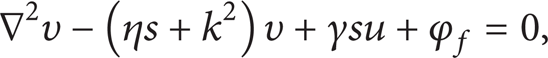
For the deformable porous medium, the displacement in the solid phase can be rewritten, in terms of velocity in the porous from (16), (17), and (18), as

u = - \frac{φ_{f}}{γ s} - \frac{1}{γ s} (\nabla^{2} - α_{2}) υ,

(34)

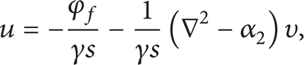
where α₂ = (ηs + k²). Substituting (34) into (16), (17), and (18) yields

[(\nabla^{2} - α_{1}) (\nabla^{2} - α_{2}) - α_{0}] υ = γ s (1 + \frac{η δ s φ_{f}}{k^{2}}),

(35)

where $α_{1} = γ s (1 + (η δ s / k^{2}))$ , α₀ = γsk². The general solution of velocity in porous medium can be expressed as

υ = A I_{0} (λ_{1} r) + B K_{0} (λ_{1} r) + C I_{0} (λ_{12} r) + D K_{0} (λ_{2} r) + \frac{γ s}{λ_{1}^{2} λ_{2}^{2}} (1 + \frac{η δ s φ_{f}}{k^{2}}),

(36)

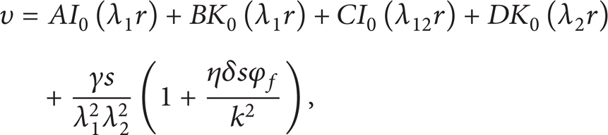
where A, B, C, and D are unknown coefficients and λ₁² and λ₂² are two distinct roots of the following quadratic equation

λ^{4} - (α_{1} + α_{2}) λ^{2} + α_{1} α_{2} - α_{0} = 0 .

(37)

From (34), the displacement of the solid phase can be written as

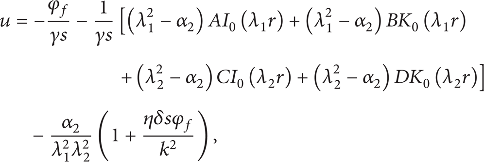
u = - \frac{φ_{f}}{γ s} - \frac{1}{γ s} [(λ_{1}^{2} - α_{2}) A I_{0} (λ_{1} r) + (λ_{1}^{2} - α_{2}) B K_{0} (λ_{1} r) + (λ_{2}^{2} - α_{2}) C I_{0} (λ_{2} r) + (λ_{2}^{2} - α_{2}) D K_{0} (λ_{2} r)] - \frac{α_{2}}{λ_{1}^{2} λ_{2}^{2}} (1 + \frac{η δ s φ_{f}}{k^{2}}),

(38)

and the velocity of pure fluid in the tube is given by

q = E I_{0} (k_{1} r) + F K_{0} (k_{1} r) + \frac{1}{k_{1}^{2}} .

(39)

Considering the boundary conditions,

r = 1: u = υ = 0,

$r = b : {(q)}_{b} = η φ_{f} {(υ)}_{b} + (η γ s / k^{2}) {(u)}_{b} = 0$ ,

$r = b : {(\partial q / \partial r)}_{b} = 1 / φ_{f} {(\partial υ / \partial r)}_{b}$ ,

$r = b : {(\partial q / \partial r)}_{b} = 1 / φ_{s} {(\partial u / \partial r)}_{b}$ ,

$r = b : 1 / φ_{f} {(\partial υ / \partial r)}_{b} = 1 / φ_{s} {(\partial u / \partial r)}_{b}$ ,

and solving (34)–(39), we have

D = \frac{I_{0} (k_{1} b) e_{0} + (1 / k_{1}^{2}) - d_{0}}{d_{1} - e_{1} I_{0} (k_{1} b)},

(40)

where

\begin{matrix} d_{0} = β_{0} υ_{0} - \frac{φ_{s} φ_{f} η}{k^{2}} + (β_{0} - \frac{φ_{s} η λ_{1}^{2}}{k^{2}}) [I_{0} (λ_{1} b) a_{0} + K_{0} (λ_{1} b) b_{0}] + (β_{0} - \frac{φ_{s} η λ_{2}^{2}}{k^{2}}) I_{0} (λ_{2} b) c_{0}, \\ d_{1} = (β_{0} - \frac{φ_{s} η λ_{1}^{2}}{k^{2}}) [I_{0} (λ_{1} b) a_{1} + K_{0} (λ_{1} b) b_{1}] + (β_{0} - \frac{φ_{s} η λ_{2}^{2}}{k^{2}}) [I_{0} (λ_{2} b) c_{1} + K_{0} (λ_{2} b)], \\ β_{0} = η (φ_{f} + \frac{φ_{s} α_{2}}{k^{2}}), \\ e_{0} = \frac{1}{φ_{f} k_{1} I_{1} (k_{1} b)} \times [λ_{1} I_{1} (λ_{1} b) a_{0} - λ_{1} K_{1} (λ_{1} b) b_{0} + λ_{2} I_{1} (λ_{2} b) c_{0}], \\ e_{1} = \frac{1}{φ_{f} k_{1} I_{1} (k_{1} b)} \times [λ_{1} I_{1} (λ_{1} b) a_{1} - λ_{1} K_{1} (λ_{1} b) b_{1} + λ_{2} I_{1} (λ_{2} b) c_{1} - λ_{2} K_{1} (λ_{2} b)], \\ a_{0} = - \frac{[υ_{0} + c_{0} I_{0} (λ_{2})] K_{1} (λ_{1} b) + h c_{0} I_{1} (λ_{2} b) K_{0} (λ_{1})}{K_{0} (λ_{1}) I_{1} (λ_{1} b) + I_{0} (λ_{1}) K_{1} (λ_{1} b)}, \\ a_{1} = - \frac{[K_{0} (λ_{2}) + c_{1} I_{0} (λ_{2})] K_{1} (λ_{1} b)}{K_{0} (λ_{1}) I_{1} (λ_{1} b) + I_{0} (λ_{1}) K_{1} (λ_{1} b)} + \frac{h [c_{1} I_{1} (λ_{2} b) - K_{1} (λ_{2} b)] K_{0} (λ_{1})}{K_{0} (λ_{1}) I_{1} (λ_{1} b) + I_{0} (λ_{1}) K_{1} (λ_{1} b)}, \\ b_{0} = - \frac{[υ_{0} + c_{0} I_{0} (λ_{2})] I_{1} (λ_{1} b) - h c_{0} I_{1} (λ_{2} b) I_{0} (λ_{1})}{K_{0} (λ_{1}) I_{1} (λ_{1} b) + I_{0} (λ_{1}) K_{1} (λ_{1} b)}, \\ b_{1} = - \frac{[K_{0} (λ_{2}) + c_{1} I_{0} (λ_{2})] I_{1} (λ_{1} b)}{K_{0} (λ_{1}) I_{1} (λ_{1} b) + I_{0} (λ_{1}) K_{1} (λ_{1} b)} - \frac{h [c_{1} I_{1} (λ_{2} b) - K_{1} (λ_{2} b)] I_{0} (λ_{1})}{K_{0} (λ_{1}) I_{1} (λ_{1} b) + I_{0} (λ_{1}) K_{1} (λ_{1} b)}, \\ c_{0} = \frac{1}{I_{0} (λ_{2})} \frac{υ_{0} λ_{1}^{2} - φ_{f}}{λ_{2}^{2} - λ_{1}^{2}}, c_{1} = - \frac{K_{0} (λ_{2})}{I_{0} (λ_{2})}, \\ h = \frac{λ_{2}}{λ_{1}} \frac{[1 + (φ_{f} / φ_{s} γ s) [λ_{2}^{2} - α_{2}]]}{[1 + (φ_{f} / φ_{s} γ s) [λ_{1}^{2} - α_{2}]]}, \\ υ_{0} = \frac{γ s}{λ_{1}^{2} λ_{2}^{2}} (1 + \frac{η δ s φ_{f}}{k^{2}}) . \end{matrix}

(41)

Finally all other coefficients are obtained by

\begin{matrix} F = 0, A = a_{0} + a_{1} D, B = b_{0} + b_{1} D, \\ C = c_{0} + c_{1} D, E = e_{0} + e_{1} D . \end{matrix}

(42)

The maximum velocity in the pure fluid occurs at the centre of the tube and may be expressed, from (39), as

q_{\max} = E + \frac{1}{k_{1}^{2}} .

(43)

By the help of (36), in particular, the general solutions can be expressed, for the velocity υ of fluid phase, when the tube is occupied completely by porous medium, is given by

υ = A^{'} I_{0} (λ_{1} r) + B^{'} K_{0} (λ_{1} r) + \frac{γ s}{λ_{1}^{2} λ_{2}^{2}} (1 + \frac{η δ s φ_{f}}{k^{2}}),

(44)

and, for the displacement u of solid phase, it is

u = - \frac{φ_{f}}{γ s} - \frac{1}{γ s} [(λ_{1}^{2} - α_{2}) A^{'} I_{0} (λ_{1} r) + (λ_{1}^{2} - α_{2}) B^{'} K_{0} (λ_{1} r) - \frac{α_{2}}{λ_{1}^{2} λ_{2}^{2}} (1 + \frac{η δ s φ_{f}}{k^{2}})],

(45)

where the constants A′ and B′ can be determined directly from the fixed boundary conditions at the rigid wall.

Following Barry et al. [2], in particular, both for steady and unsteady flows, we can prove that at the interface when ∊_T → 0 the velocity has behavior

q = k_{T} \frac{\partial q}{\partial n},

(46)

where k_T is a constant and n is the normal to the interface.

6. Results and Discussions

The results for steady state flows are shown in Figures 2, 3, and 4. Normalized velocity at the centre of the tube q_max in (26) is plotted in Figures 2 and 3. Figure 2 shows the variation of velocity with the porous layer thickness ∊_T ∊ [0, 1], when φ_f = 0.6, and Figure 3 shows the variation of velocity with the volume fraction φ_f ∊ [0, 1], when ∊_T = 0.3. These results indicate that the velocity in the fluid decreases as the thickness increases for constant porosity of the layer and the maximum velocity increases when the porosity increases for constant thickness.

Figure 2:

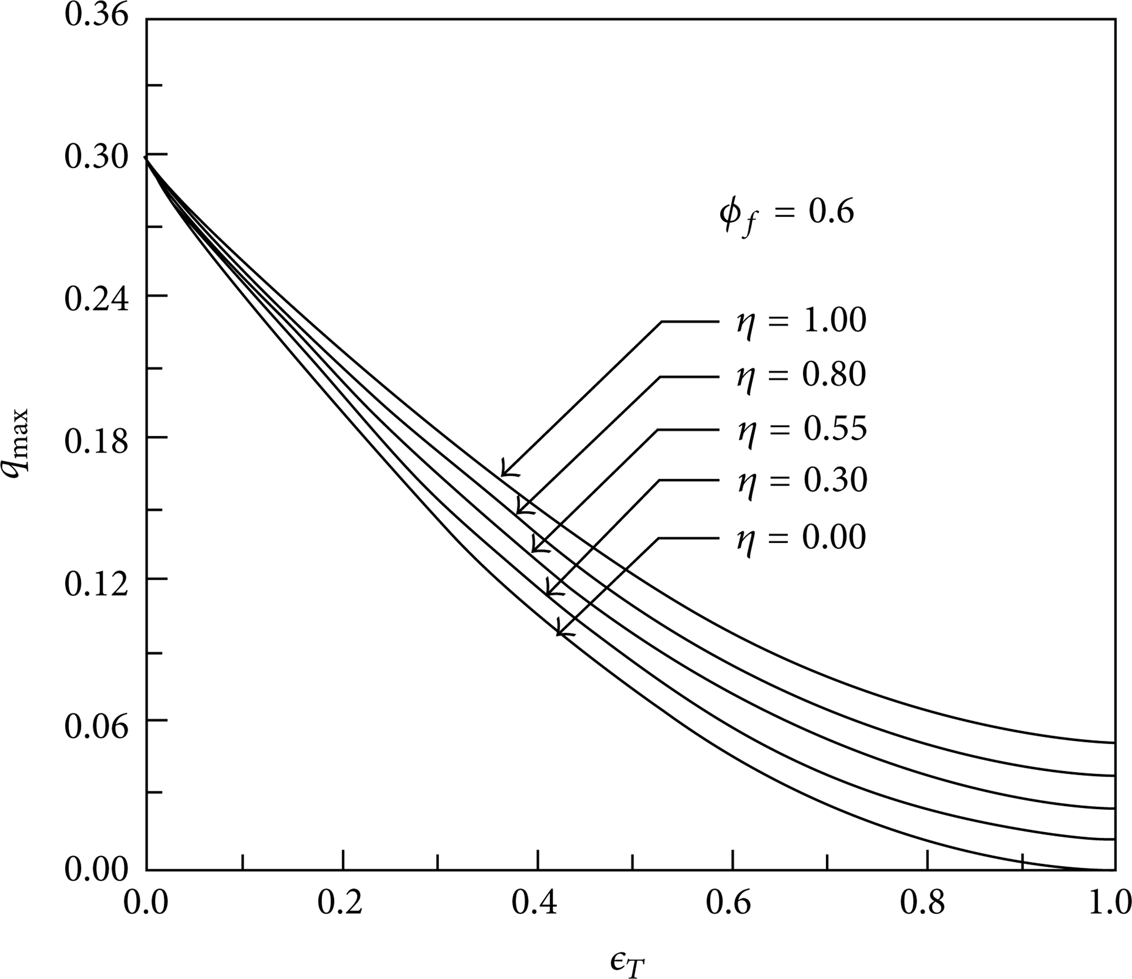
Variation of maximum velocity (q_max) with ∊_T ∊ [0, 1], when φ_f = 0.6, k² = 2.

Figure 3:

Variation of maximum velocity (q_max) with φ_f ∊ [0, 1], when ∊_T = 0.3, k² = 2.

Figure 4:

Fluid flux profile in the tube and in the porous medium with the parameters ∊_T = 0.3, η = 0.6, and k² = 2.

The solutions for the displacement (u) of solid phase and the velocities of fluid (υ, q) in (23), (24), and (25) are plotted in Figure 4 for the porosity φ_f = 0.6 and 0.9, respectively, where the parameters are selected as ∊_T = 0.3, η = 0.6, and k² = 2. In the case of steady state flow, the velocity profile in the pure fluid is parabolic plus a uniform flow; the fluid flux profile φ_fυ_r^f in porous medium and the displacement of the solid phase u are almost linear. By increasing the porosity of the two-phase medium, the velocities of both fluids in the pure fluid and the porous medium increase as there is less solid to impede the flow. Therefore, the displacement of solid decreases, since there is less drag on the solid component.

The solutions of maximum velocity in the pure fluid in time domain are shown in Figure 5, when parameters φ_f = 0.6, η = 0.6, and k² = 2 are applied to the system under the pressure gradient g(t) = H(t), where H(t) is the Heaviside (step) function. It is apparent that the maximum velocity decreases when the thickness of the porous medium ∊_T increases. As expected, the velocity converges rapidly to the steady state solutions in (26), that is, immediately after the normalised time t > 1. Figure 6 demonstrates how the flow develops from a suddenly applied acceleration to the final steady state when the values of the chosen parameters are ∊_T = 0.3, η = 0.6, and k² = 2. The effects of the porosity and the rigid wall of the tube on the velocity profile in pure fluid are displayed for different volume fraction φ_f = 0.6 and 0.9.

Figure 5:

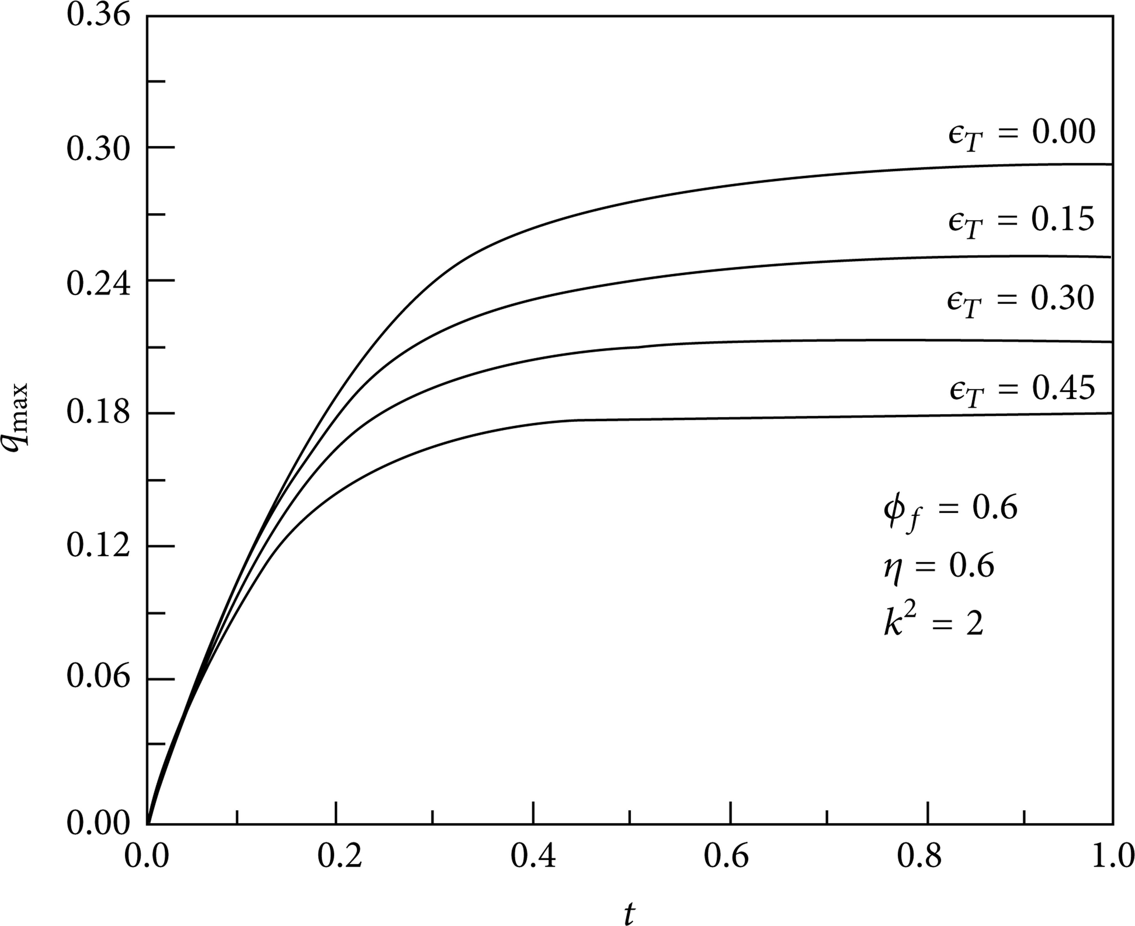
Maximum velocity variation with different values of thickness of porous medium. The parameters are selected as φ_f = 0.6, η = 0.6, and k² = 2.

Figure 6:

Velocity profile at five times: t = 0.06, 0.12, 0.24, 0.48, and 1 for porosity φ_f = 0.6 and 0.9.

For deformable porous medium, the maximum velocity in the pure fluid is shown in Figure 7 when the parameters are chosen as φ_f = 0.6, η = 0.6, k² = 2, and γ = 0.6. The effect of porous layer thickness becomes significant in this case. We notice that, for large thickness of porous layer (∊_T > 0.3), the velocity at the centre of the tube oscillation occurs at the position of the steady state flow solution. It is believed that such oscillation in the fluid is caused by the vibration of solid phase around the equilibrium position under dynamic pressure gradient. To illustrate such influence, we plot the variation of displacement of the solid phase at the interface against the real time in Figure 8. Furthermore, the dynamic response for the maximum velocity of the pure fluid subjected to a sinusoid pressure gradient is shown in Figure 9.

Figure 7:

The velocity at the centre position in pure fluid with parameters φ_f = 0.6, η = 0.6, k² = 2, δ = 3, and γ = 0.6.

Figure 8:

The displacement of the solid phase at the interface with parameters φ_f = 0.6, η = 0.6, k² = 2, δ = 3, and γ = 0.6.

Figure 9:

The maximum velocity in pure fluid under the sinusoid pressure gradient when parameters φ_f = 0.6, η = 0.6, k² = 2, δ = 3, and γ = 0.6 are applied.

7. Conclusion

General solutions for the displacement of solid phase and the velocities for both fluids in the porous layer and in the pure fluid space are obtained. The connection (jump) conditions at the interface between porous medium and pure fluid discussed for steady viscous flow are introduced for unsteady viscous flow. It is considered that for unsteady flow the volume-average velocity in the tangential direction is continuous across the porous interface and the stress distribution is proportional to itsvolume fractions at the interface. The interaction for the solid and the fluid phases in the porous medium and the effect on the velocity in the pure fluid are investigated in detail for three cases with different solid phases: (i) steady state deformation; (ii) rigid porous layer; (iii) deformable porous layer. Durbin's Laplace transformation inversion algorithm is used to obtain a high accuracy solution in the real time domain. Sufficient examples are given for Heaviside and sinuous pressure gradients applied to the system. The derived analytical solutions can be used to test some interesting practical problems. These analytical solutions are derived for axial symmetric problems.

Footnotes

Nomenclature

Acknowledgment

The authors are grateful to both referees for their valuable suggestions and comments for the improvement of this paper.

References

Richardson

and Power

, “A boundary element analysis of creeping flow past two porous bodies of arbitrary shape,” Engineering Analysis with Boundary Elements, vol. 17, no. 3, pp. 193–204, 1996.

Barry

S. I.

Parkerf

K. H.

, and Aldis

G. K.

, “Fluid flow over a thin deformable porous layer,” Zeitschrift für Angewandte Mathematik und Physik, vol. 42, no. 5, pp. 633–648, 1991.

Barry

S. I.

Mercer

G. N.

, and Zoppou

, “Deformation and fluid flow due to a source in a poro-elastic layer,” Applied Mathematical Modelling, vol. 21, no. 11, pp. 681–689, 1997.

Pozrikidis

, Boundary Integral and Singularity Method for Linearized Viscous Flow, Cambridge University Press, Cambridge, UK, 1992.

Wrobel

L. C.

, “The boundary element method,” in Applications in Thermo-Fluids and Acoustics, vol. 1, John Wiley & Sons, Hoboken, NJ, USA, 2002.

Dwivedi

J. P.

Singh

V. P.

, and Lal

R. K.

, “Stress, displacement and pore pressure of partially sealed circular tunnel surrounded by viscoelastic,” Advances in Theoretical and Applied Mechanics., vol. 4, no. 1–4, pp. 189–198, 2011.