
Abstract
Any trajectory calculation method has three primary sources of errors, which are model error, parameter error, and initial state error. In this paper, based on initial projectile flight trajectory data measured using Doppler radar system; a new iterative method is developed to estimate the projectile attitude and the corresponding impact point to improve the second shot hit probability. In order to estimate the projectile initial state, the launch dynamics model of practical 155 mm self-propelled artillery is defined, and hence, the vibration characteristics of the self-propelled artillery is obtained using the transfer matrix method of linear multibody system MSTMM. A discrete time transfer matrix DTTM-4DOF is developed using the modified point mass equations of motion to compute the projectile trajectory and set a direct algebraic relation between any two successive radar data. During iterations, adjustments to the repose angle are made until an agreement with acceptable tolerance occurs between the Doppler radar measurements and the estimated values. Simulated Doppler radar measurements are generated using the nonlinear six-degree-of-freedom trajectory model using the resulted initial disturbance. Results demonstrate that the data estimated using the proposed algorithm agrees well with the simulated Doppler radar data obtained numerically using the nonlinear six-degree-of-freedom model.
1. Introduction
There are different computation methods to estimate the projectile ballistic trajectory and subsequent impact point. These methods have three primary sources of errors, which are model error, parameter error, and initial state error. The model error depends on how much the projectile equations of motion are simplified. Increasing model complexity means decreasing model error, but the parameter and initial state errors will increase [1]. In 1964, the projectile six-degree-of-freedom (6-DOF) equations of motion in terms of direction cosines [2] was developed by the ballistic research laboratory, which is the most accurate model that can simulate the rigid body flight dynamics under the condition that all the aerodynamic forces and moments, and the initial state, are known to a high degree of accuracy. Using this system of equations, a discrete time transfer matrix method DTTM-6DOF [3] has been developed to accurately compute the projectile ballistic trajectory and minimize the corresponding computational time.
During testing new weapons, an accurate instrumentation is needed to measure the in-flight projectile parameters. Projectiles do not have enough space to install on-board sensors to acquire these parameters. Further, considering the severe environment faced by the projectile during flight such as velocity and spinning rate, a low cost and accurate measurement method is required. The most promising method is using a Doppler radar system [4] due to its robustness, portability, accuracy, and providing nearly continuous velocity-time information on the projectile during the flight down range. A number of authors presented different algorithms based on Doppler radar measurements. In 1958, Shapiro [5] proposed three different estimation methods to compute the six parameters that define the orbital parameters describing the ballistic missile trajectory using single radar measurements which include range, range-rate, and the azimuth and elevation angles. These methods are the maximum likelihood, the weighted least squares, and a deterministic method. In 1985, a new iterative method had been developed [6] and applied to a modified version of 6-DOF model to extract actual thrust made during the flight of rocket-assisted projectiles using Doppler radar measurements. In 2008, an iterative algorithm had been developed [7] using maximum likelihood method to predict the drag characteristics of projectiles in motion by processing data acquired by Doppler radar system, where the point mass model was used due to the projectile small angle of attack along the trajectory.
The movements of artillery and projectile are very complex in launch process because of the complex structure of self-propelled artillery and the severe environments, such as, high temperature, high pressure, high speed, instantaneous state, multibody, and mutation, in launch process [8]. Therefore, gun launch dynamics has a primary concern in designing embedded navigation and guidance systems in case of guided projectiles and evaluating the projectile initial disturbance in case of unguided projectiles. In 2000, the launch dynamics of self-propelled artillery [9] based on transfer matrix method of multibody system MSTMM was developed for studying the vibration characteristics and dynamics of self-propelled artillery and the projectile's initial disturbance. In 2001, a finite element analysis [10] had been done for the breech closure for the 155 mm Cannon M199, which is normally mounted on the Towed Howitzer M198. The analysis is for a 9 body problem with 13 contact surfaces and was solved for both static and dynamic load cases. In 2004, a simplified model [11] had been done to predict joint forces and accelerations along the length of a simplified 155 mm projectile using modal superposition. These predicted loads used to locate all guidance equipment, sensors, joints, and computers that must operate reliably after exiting the gun. In 2005, a sophisticated 3D-finite-element model [12] had been developed to investigate the survivability of embedded electrical systems by simulating the launch dynamics of a surrogate Excalibur projectile. This study determined free mounting locations trouble for sensitive components and parametric investigation in identifying sensitive factors affecting the muzzle-exit motion of projectile substructures. In 2008, a new method [13] named as transfer matrix method of linear multibody system MSTMM for linear hybrid multibody system dynamics was developed. This method had been applied to a Multiple Rocket System as a linear multi-rigid-flexible-body system. In 2011, the dynamics problem of a shipboard gun system had been solved [14] using the discrete time transfer matrix method of multibody system MSDTTMM [15].
In this paper, an iterative method is developed to determine the projectile kinematics including attitude and angular motion using Doppler radar measurements. Doppler radar measurements are only available during the first portion of projectile trajectory including the range, the range-rate, and the azimuth and elevation angles (position and velocity vectors), in order not to be recognized by the enemy counterattack systems. Simulated Doppler radar measurements are generated during flight time using 6-DOF trajectory model including the projectile initial disturbance problem. The projectile initial disturbance is computed by solving the self-propelled artillery and projectile dynamics as a multi-rigid-flexible system using Transfer Matrix Method of Multibody System MSTMM [8], where the overall transfer equation of self-propelled artillery was obtained to compute the corresponding vibration characteristics. In order to iteratively compute the projectile attitude, a discrete time transfer matrix DTTM-4DOF is developed based on linearization of the nonlinear modified point mass equations of motion using second-order Taylor series [16]. The system state vector, which defines the projectile trajectory parameters during Doppler radar observations, is defined by 13 state variables, which are the projectile position, velocity, spin rate, repose angle, and wind velocity. During iterations, adjustments to the repose angle are made until agreement with a certain tolerance occurs between the Doppler radar velocity measurements and the value predicted using DTTM-4DOF. Finally, projectile impact point can be predicted precisely depending on the length of radar data available, where the data estimated at the end of radar observations is used as an initial state to the 6-DOF trajectory model.
2. Launch Dynamics Model for Self-Propelled Artillery System
To accurately estimate the projectile initial state, launch process has to be decided precisely by studying the artillery and projectile dynamics from the moment of firing to the state of muzzle point. Four interactions have to be considered, the interaction between projectile and artillery, the interaction between the artillery transverse and longitudinal motion, the interaction between rigid and flexible body, and, finally, the interaction between space coordinate and time coordinate for describing motion parameters.
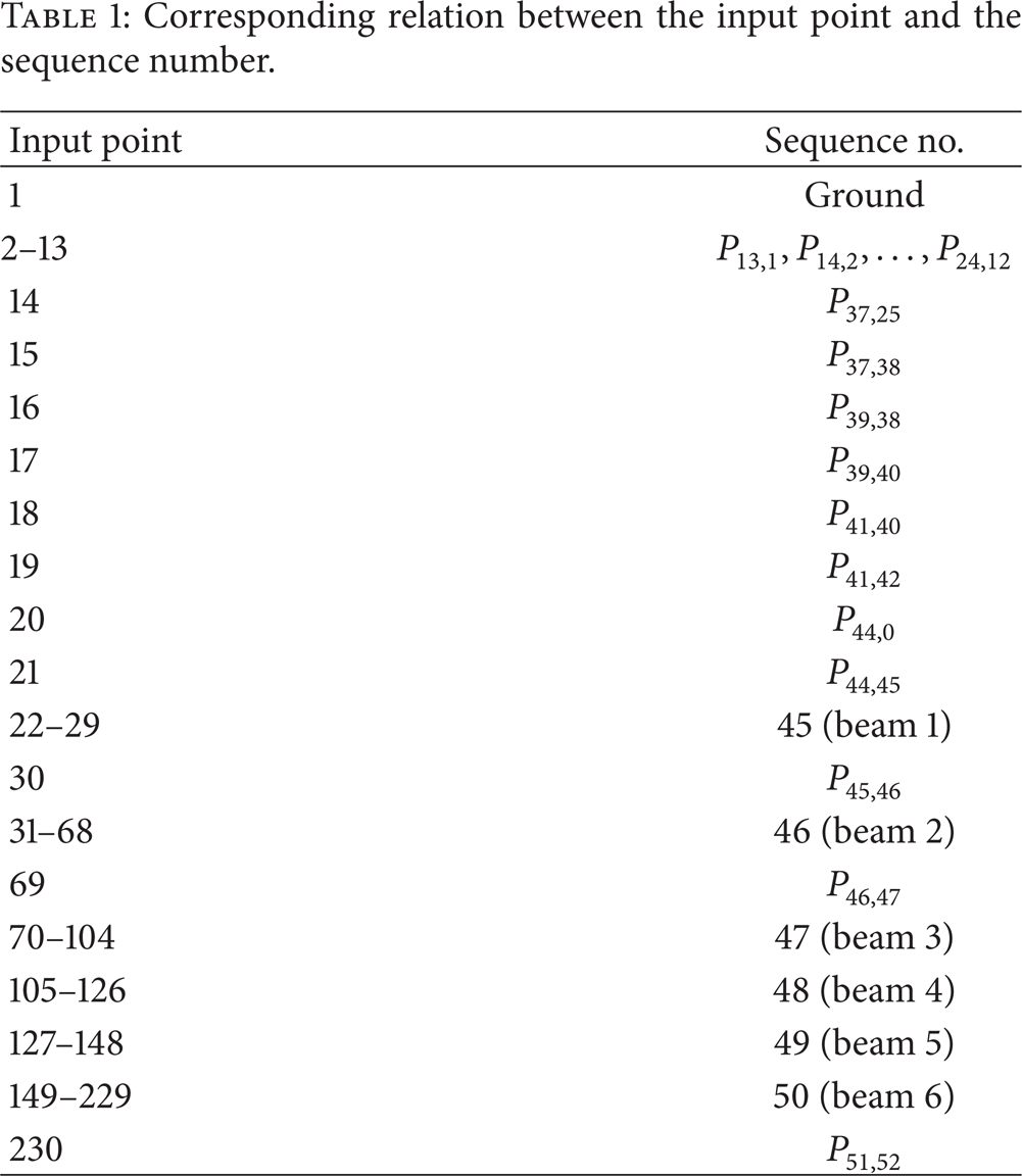
The launch dynamics model of self-propelled artillery is a multi-rigid-flexible system which has been studied in [8]. This system is composed of 51 elements (23 bodies and 28 joints) as shown in Figure 1. It has 3 boundary ends including ground, gun breech, and muzzle. The ground (0) is regarded as an infinity rigid body and the first input point, the gun breech (44) is regarded as rigid body and the second input point, and the muzzle (52) is the output point. The road wheels (13–24) are regarded as lumped masses. The hull (37), revolving part (39), elevating part (41), and muzzle brake (51) are regarded as rigid bodies; the barrel is divided into 6 segments (45–50) and each is regarded as a beam with equal sectional area. The interactions (1–12) between ground and road wheel and the connections (25–36) between road wheel and the hull are, respectively, modeled with springs and dampers in 3 directions. Connections (38, 40, 42, and 43) are modeled with springs and rotary springs accompanying dampers to represent relative linear motion and relative angular motion in 3 directions at the same time. All connections between barrel and gun breech, barrel and muzzle brake, and each segment of barrel are regarded as fixed. The masses of traversing mechanism, elevating mechanism, and equilibrator fall into elevating part, revolving parts, and hull, respectively. According to the launch dynamics model of self-propelled artillery and the sequence number of each element, there are 49 connection points which are Pi, i – 12, Pi, i + 12 (i = 13–24), P37, i (i = 25–36), P37,38, P39,38, P39,40, P41,40, P41,42, P41,43, P44,45, P45,46, P46,47, P47,48, P48,49, P49,50, and P51,50 and 14 boundary points which are P0, i (i = 1–12), P44,0, P51,52, respectively. The overall transfer equation of the practical 155 mm self-propelled artillery shown in Figure 1 was obtained using the transfer matrix method of linear multibody system MSTMM [8].
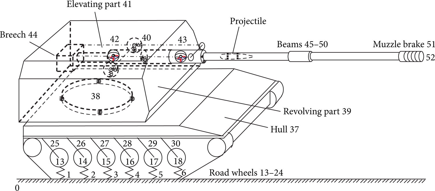
Launch dynamic model of self-propelled artillery [8].
During launch process, all forces and moments acting between barrel and elevating part, elevating part and revolving part, revolving part and the hull, the hull and road wheels, and road wheels and the ground are regarded as internal forces. The forces that acted on the barrel by projectile [8, 17] and the forces that acted on the barrel and muzzle brake by propellant gas [8] are regarded as external forces of the artillery. The recoil resistance between the barrel and elevating part produced by recoil and counter-recoil mechanism is decomposed into external force and internal force, and the internal force is proportional to the relative displacement between barrel and elevating part.
3. Projectile Flight Trajectory Model
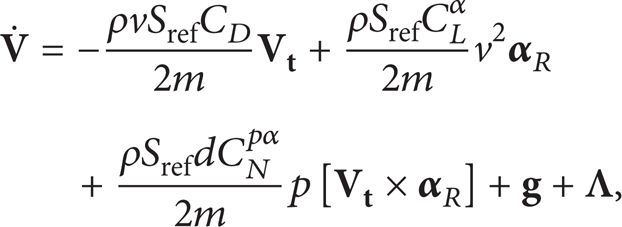
Due to the complexity of projectile initial disturbance determination, a modified point mass 4-DOF model for an unguided rigid projectile was stated in [18, 19]. These equations assume that the epicyclic pitching and yawing motion of the projectile are small everywhere along the trajectory; therefore, the yaw and pitch moments considered in 6-DOF trajectory model [19] are neglected.
The projectile modified point mass equations of motion with respect to earth fixed coordinate system (X1, X2, X3) as shown in Figure 2 are given by [19]


where C
D
, C
L
α, C
N
pα, and C
l
p
are the aerodynamic drag force, lift force, Magnus force, and spin damping moment coefficients, respectively;

Coordinate system and directions of ballistic target.
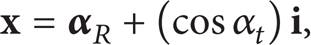
The projectile repose angle

where
And the total aerodynamic angle of attack is [3, 18, 19]
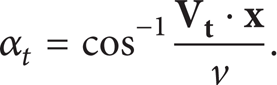
The simplified form of the repose angle is given by [19]
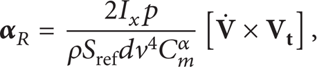
where C m α is the aerodynamic pitching moment coefficient.
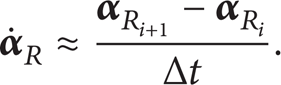
For discrete systems, a good approximation was done for the projectile repose angle [20] as

The Coriolis acceleration due to earth's rotation and gravitational acceleration are given by [3, 19]
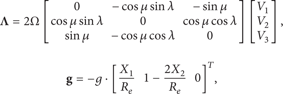
where g = g o · [1 – 0.0026 cos(2μ)], g o = 9.80665 m/s2; Ω is the earth's angular velocity; μ, λ are the corresponding latitude and longitude of the firing sight; and R e is the average radius of the earth (−6356766 m).
Due to spherical earth approximation, the instantaneous projectile altitude H is defined as [19]
4. Discrete Time Transfer Matrix for Modified Point Mass Equations of Motion
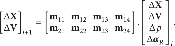
To develop a discrete time transfer matrix DTTM-4DOF using the modified point mass equations of motion mentioned above, a system state vector

DTTM-4DOF is the relation between any two successive state vectors, where

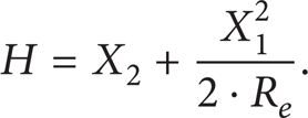
The 2nd-order Taylor series is given by [16]

where

The equations of motion matrix

where
All elements of matrix

where g
X
2
= g/X2,

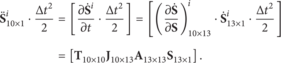
where
where a1 = (Sref/2m), a2 = ((Srefd)/2m), b1 = ((Sref · d2)/(2 · I x )), b2 = (d/b1), and anjan65.
The change in wind velocity vector with the projectile position

The Jacobian matrix

The partial derivatives of the projectile acceleration in (2) with respect to wind velocity and projectile velocity are given by

where

Similarly, using (3), the rate of change of projectile spin rate with respect to its velocity is given by

The partial derivatives of the projectile yaw of repose in (7) with respect to projectile velocity and spin rate are as follows:

where
The time matrix

By Applying (14), (19), and (25) into (12), the overall discrete time transfer matrix is given by

where,


All elements
5. Projectile Attitude Determination Algorithm
The algorithm presented here is an iterative method to compute (1) the projectile muzzle velocity and line of sight by using the first projectile displacement observed by radar, and (2) the projectile flight attitude and the corresponding angular momentum by using the Doppler velocity observed by radar. At each time step, the difference between the data measured by radar and the estimated parameters by using DTTM-4DOF are linearly related as follows:
At the beginning of flight time, the initial guess of the projectile velocity

The projectile muzzle spin rate is corrected by adding Δp
o
using the velocity difference Δ

where n is the gun twist rate.
At the beginning of each iteration cycle, the DTTM-4DOF matrix is computed and hence the projectile states


Then, the estimated parameters are used as initials for the next time step.
As shown in Figure 3, during each time step, the projectile attitude and the corresponding angular momentum can be estimated using the following procedure.
The projectile total angle of attack can be computed by

The projectile's axis of symmetry unit vector
where
The rate of change of the projectile total velocity unit vector is given by [19]

Due to the small variation in projectile repose angle during flight [19], its rate of change is approximated to be linear during each time step as
The rate of change of projectile's axis of symmetry unit vector

The projectile angular momentum divided by I y in earth fixed coordinate is given by [19]


Projectile attitude and impact point determination flow chart.
6. Simulated Trajectory Generation
In order to validate the proposed algorithm, a simulated noiseless ballistic trajectory for 155 mm high explosive HE spin stabilized projectile is generated to simulate the Doppler radar velocity measurements data. The projectile mass, length, center of mass measured from the nose, and the axial and transverse mass moments of inertia are 46.5 kg, 0.902 m, 0.593 m, 0.1585 kg/m2, and 1.8816 kg/m2, respectively. This trajectory is generated using the nonlinear 6-DOF trajectory model [2, 19] including projectile initial disturbance problem with 52° firing elevating angle.
6.1. Natural Vibration Characteristics of the Self-Propelled Artillery
To compute the vibration characteristics for 155 mm self-propelled artillery, the input points corresponding to sequence numbers of connection points and elements shown in Figure 1 are identified in Table 1.
Corresponding relation between the input point and the sequence number.
All simulation and test results of natural frequencies for the first sixteen ranks are listed in [8], where the simulation results have a good agreement with that obtained by experiments. Figures 4 and 5 show part of the resulted system mode shapes, where the 1st mode mainly represents the recoil motion of barrel, the 2nd mode represents the horizontal revolving motions of turret, cradle, and barrel, the 3rd mode mainly represents the elevating motions of cradle and barrel, and the 16th mode mainly represents the transverse motion of barrel and complex motions of other elements. The low rank mode shapes do not represent the transverse elastic deformation of the barrel that is only represented in high rank [8].

The 1st and 2nd mode shapes in X- and Z-direction, respectively.

The 3rd and 16th mode shape in Y-direction.
6.2. Computation of Projectile Initial Disturbance
The resulted projectile launch dynamics parameters with respect to gun tube coordinate system are shown in Figures 6–10. The gun tube coordinate system O3x O y O z O is defined as follows: the origin O3 is the intersection point between axis of gun tube and the vertical plane of projectile's axis of symmetry, the x O -axis is along gun tube axis of symmetry and points to muzzle, the y O -axis (plumb direction) is vertical to x O -axis and points up, the direction of z O -axis (swing direction) is determined by the right-hand role. The projectile longitudinal displacement, velocity, and acceleration with respect to gun tube axis are shown in Figures 6 and 7, where L b is the total barrel length. Figure 8 shows the projectile center of gravity plumb and sidewise displacement with respect to gun tube axis as function of nondimensionalized longitudinal displacement.

Projectile longitudinal displacement.
Projectile longitudinal velocity and acceleration.
Projectile lateral displacement.

Projectile angular displacement during launch.
Projectile angular velocity during launch.
The projectile axes orientation with respect to line of sight LOS, which includes the projectile roll, plumb and sidewise swing components, angular displacement, and velocity, are illustrated in Figures 9 and 10, respectively. The corresponding projectile angular displacement and velocity components at muzzle are shown in Table 2, where the deflection angle is the angle between the projectile velocity vector and LOS while projectile is just flying off from muzzle, and the swing angle is the angle between projectile axes and LOS at the same moment.
Simulation results of initial disturbance of projectile.
The projectile initial flight conditions corresponding to the self-propelled artillery launch dynamics, and hence, the projectile initial disturbance calculations proposed before are listed in Table 3, which include the projectile initial velocity V1, V2, V3, initial roll p, pitch q and yaw r rates, initial angle of attack α, and side-slip angle β.
Simulation results of the projectile parameters at muzzle.

7. Estimation Results
A computer program has been developed by using the nonlinear 6-DOF dynamic equations stated in [19]. All simulations were computed with fixed time step size of 0.001 s and integrated using Runge-Kutta-Gill method.
Firstly, a simulated noiseless Doppler radar velocity measurements data 6DOF-R are generated, including the projectile's position and velocity vectors, using the initial flight conditions listed in Table 3. The Doppler radar output data frequency is assumed to be 100 Hz. The 6DOF-R data is assumed to be the real projectile trajectory data. The corresponding impact point range, drift, maximum altitude, velocity, and flight time are 19689.2 m, 1027.85 m, 8180.9 m, 338.76 m/s, and 81.932 s, respectively.
Secondly, a nondisturbed trajectory simulation has been performed as nominal trajectory 6DOF-N, where the initial flight conditions used are 700 m/s, 52°, and 1279.7 rad/s for muzzle velocity, elevating angle, and spin rate, respectively. The corresponding impact point range, drift, maximum altitude, velocity, and flight time are 19729 m, 995 m, 8162 m, 338.66 m/s, and 81.829 s, respectively.
Finally, the iterative algorithm shown in Figure 3 has been applied to estimate the projectile attitude, using the generated Doppler radar data 6DOF-R, where the initial flight conditions are as the data used to simulate the projectile nominal trajectory 6DOF-N. Figures 11, 12, and 13 show that the estimated projectile velocity, AOA, and attitude, respectively, are matching very well with the simulated Doppler radar trajectory 6DOF-R, although the nominal (non-disturbed) trajectory results 6DOF-N are mismatching the 6DOF-R. Figures 14 and 15 show the rate of change of the projectile AOA and attitude, respectively, during flight time, where the estimated values are matched very well with 6DOF-R except at some peaks/dips data points due to the large difference between the data frequency obtained from radar and the simulation speed of the real trajectory data (1: 10). Therefore, the final estimated value shown in Figure 16, which represents the projectile angular momentum per-unit I y has mismatched with 6DOF-R data during these peaks/dips data points.

Projectile velocity vector versus flight time.

Projectile total angle of attack vector versus flight time.
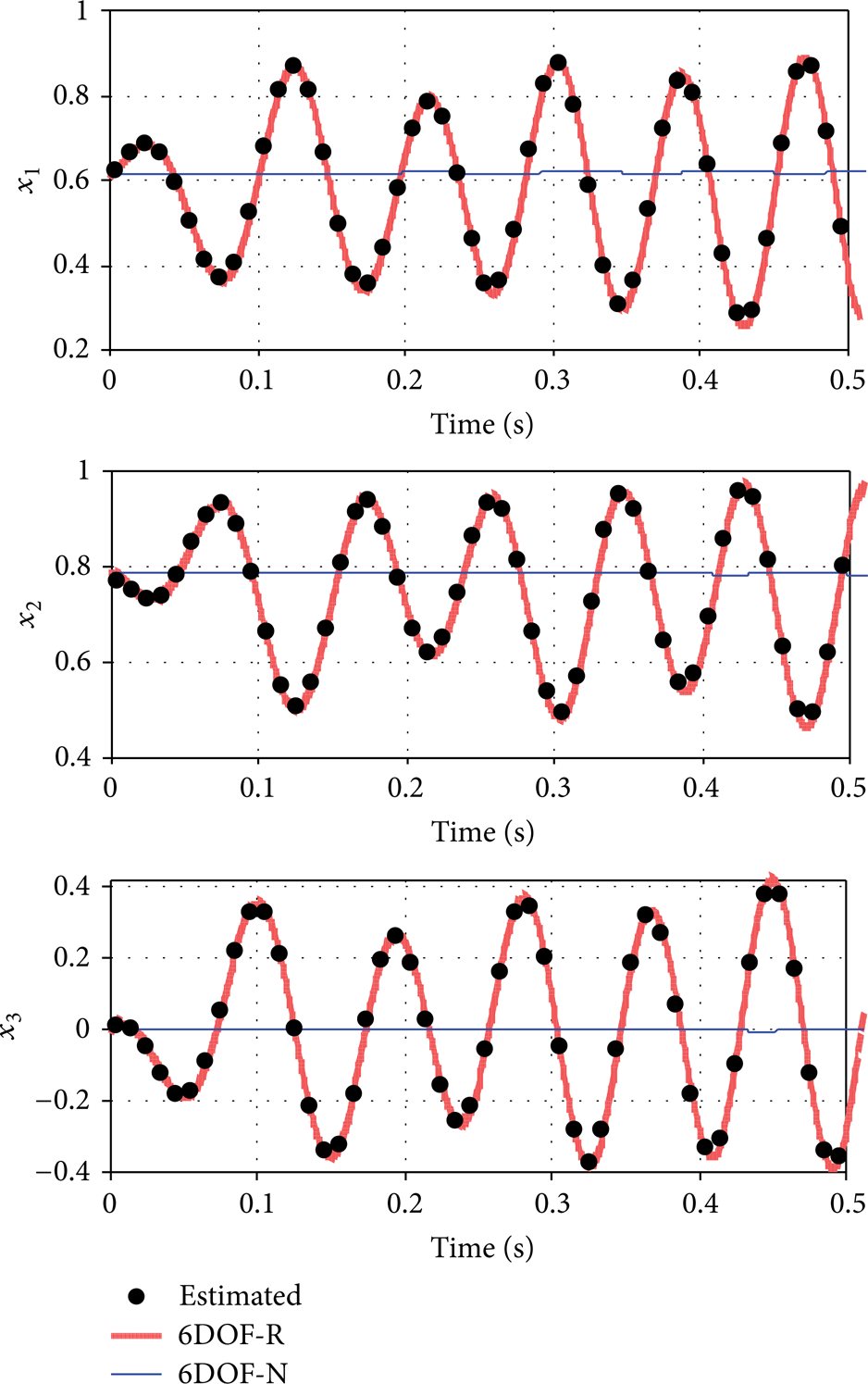
The projectile's axis of symmetry unit vector.

Rate of change of the projectile AOA.

Rate of change of the projectile's axis of symmetry unit vector.

Projectile angular momentum per unit I y .
For nominal trajectory data 6DOF-N, the impact range ∊ R and drift ∊ D errors relative to 6DOF-R are 0.202% and −3.2%, respectively. All impact point parameters inaccuracies for the proposed algorithm as function of simulated Doppler radar data availability are shown in Figure 17, where these errors, ∊ R and ∊ D , can be reduced by approximately 8 and 7 times, respectively, as the radar data is available for the first 10% of total flight time and approximately by 10 and 70 times to be −0.0205% and −0.0448%, respectively, as the radar data availability is 15% of total flight time.

Impact range and drift error versus Doppler Radar data availability.
8. Conclusion
The main objective of this paper is determining the effect of self-propelled artillery dynamics on the projectile impact point prediction accuracy, and hence, an iterative projectile attitude determination algorithm was developed to accurately compute the projectile ballistic trajectory and the corresponding impact point parameters by using a Doppler radar data. The projectile initial disturbance was computed by solving the interaction between the self-propelled artillery and the projectile dynamics during launch process. A discrete time transfer matrix DTTM-4DOF was developed by linearizing the projectile nonlinear modified point mass equations using second-order Taylor series. The main advantages of using DTTM-4DOF are (1) linearly relating any two successive radar data, and (2) increasing the computation speed due to solving a set of algebraic equations instead of using traditional numerical methods. An iterative projectile attitude determination algorithm was developed to accurately compute the projectile ballistic trajectory and predict the impact point parameters by using a Doppler radar data. In order to validate the proposed algorithm, a simulated noiseless trajectory data was generated as Doppler radar velocity measurements data 6DOF-R for 155 mm HE spin stabilized projectile using the nonlinear six-degree-of-freedom trajectory model including projectile initial disturbance problem. A nominal ballistic trajectory 6DOF-N was generated with 52° firing elevating angle and without including the effect of launch dynamics to show the importance of the projectile initial disturbance. Based on the results obtained, the proposed algorithm estimated the projectile velocity and attitude very well compared to the 6DOF-R trajectory data. The impact range and drift inaccuracies were reduced from 0.202% and −3.2% in case of nominal trajectory 6DOF-N to be −0.0205% and −0.0448% by applying the proposed algorithm as the radar data availability is 15% of total flight time. As the projectile dynamic stability increased, the radar data availability can be decreased. Finally, the proposed algorithm can estimate the projectile impact point accurately without computing the projectile initial disturbance, where different projectiles have different initial disturbances based on many factors, such as, gun barrel wear and erosion, projectile initial position and attitude inside barrel, and the propellant charge amount, composition, and homogeneity.
Footnotes
Appendix
Acknowledgments
The research was supported by the Research Fund for the Doctoral Program of Higher Education of China (20113219110025), the Natural Science Foundation of China Government (11102089), and the Program for New Century Excellent Talents in University (NCET-10-0075).