Fault Prognostic Based on Hybrid Method of State Judgment and Regression

Abstract

Fault prognostic is one of the most important problems in equipment health management system. This paper presents a hybrid method of mixture of Gaussian hidden Markov model (MG-HMM) and fixed size least squares support vector regression (FS-LSSVR) for fault prognostic. The system is established based on three parts. The first part trains the MG-HMM and FS-LSSVR model. According to the known samples, several MG-HMM models can be learned based on expectation maximization (EM) algorithm. Then, the forward variables can be calculated based on these MG-HMM models. Based on these forward variables, the corresponding FS-LSSVR models are built. All the MG-HMM models and corresponding FS-LSSVR models are combined into a model library. The second part recognizes the unknown sample based on the model library. This part obtains the MG-HMM model and FS-LSSVR model by maximization likelihood calculation between the unknown sample and MG-HMM models. The third part of the system calculates the forward variables based on the MG-HMM obtained from the second part. These forward variables are inputted into the corresponding FS-LSSVR model to compute the remaining useful life (RUL) of the unknown sample. Finally, we carry out experiments on benchmark data set to verify the proposed method. The results illustrate the effectiveness of the hybrid method.

1. Introduction

RUL is one of the most important problems in many application areas such as condition based maintenance (CBM) [1], fault prognostics (FP) [2], and prognostics and health management (PHM) system [3]. Obviously, the RUL of a system or a component is a random variable. Three techniques are applied to estimate the RUL: life cycle model, expert knowledge system, and data-driven model [4]. The data-driven model compromises the merits of adaptability, low cost, and little expert knowledge. For these reasons, it has been widely concerned in recent years.

Many artificial intelligence (AI) techniques have been applied to fault prognostic. Expert system (ES) is a computer system which consists of a knowledge database and an inference mechanism. The knowledge database contains domain knowledge for the solution of problems. This approach is not best for situations where there is a lack of expert knowledge [5]. ES cannot handle new situations not covered explicitly in its knowledge database. Fuzzy logic can represent uncertainty of complexity system while it is no feasible where there is no suitable membership function [6]. Artificial Neural Network (ANN) can simulate the structures and functions of biological neural networks. This approach can capture potential knowledge from input patterns. However there is no standard method to determine the structure of the network [7]. Support vector machine (SVM) project feature space into a higher dimensional space by a kernel function and finds an optimized separation surface in the higher dimensional space. This approach can achieve better generalization capability than ANN while there this no standard kernel function selection method for SVM [8].

Hidden Markov model (HMM) has demonstrated its superior performance in lots of application areas, such as speech recognition and gesture recognition. It is more suitable for modeling on stationary stochastic signal. Meanwhile, HMM is also inspected and applied into fault diagnosis or fault prognostics [9]. Comparing with many other RUL estimation methods, a distinct advantage of the HMM model is that HMM model can give an intelligible explanation. Bunks et al. firstly put forward a HMM model built on the Westland helicopter gear monitoring data, and then the RUL of gear is estimated based on the HMM model [10]. In this paper, the authors estimate each of the 68 operating conditions with a different eight-dimensional Gaussian model. At the same time, they make hypothesis that the health state could not revert once it departs from the current health state during its operation. Baruah and Chinnam apply HMM to model the metal cutting tools [11, 12]. The proposed method can simultaneously meet the requirements of fault diagnosis and fault prognostics. To describe a three-state transition procedure, a two-mixture Gaussian model is used for modeling. Based on the previous model, once the previous state transition time is known, the next state transition time can be estimated. Camci and Chinnam make a thorough inspection on drill bit health evaluation [13]. They define the drill bit health level as drilling holes number. Each drilling history time series can be used to train a separate HMM model. These HMM models are used to estimate the drill bit health in time. Then a hierarchy HMM is established to model the state transition relation in which the upper HMM model describes the drill bit health state transition relationship while the lower HMM model describes the drilling time series emitted from one state in the upper HMM model. Once the drill bit health is determined, the RUL is calculated based on the probability transition matrix in the upper HMM model. Ocak et al. make a decomposition on the bearing vibration signals by using wavelet packet technique. The Nth layer node data is used as feature vector for HMM training. If the bearing state need to be judged, the HMM models will be applied into likelihood calculation. The experimental results found that, as the bearing wears, the likelihood gradually drops [14]. Tai et al. apply HMM model into condition monitoring of nozzle [15]. Zhou et al. combine the HMM model and belief rule base under a variable circumstance, where belief rules are used to model the dynamic environment. Eventually, fault diagnosis and fault prognostics are implemented for the complex system based on this mixture model [16]. Tobon-Mejia et al. establish the models on the bearing data with mixture of gaussian hidden Markov model (MG-HMM). Once a sequence classification is determined, a graph-based path traversal algorithm is carried on to estimate the RUL of bearing [17]. Liu et al. present a hybrid method of HMM and LSSVR to predict the RUL. The LSSVR is used to predict the future features based on the past samples and the HMM is used to judge the future state according to the future predicted features [18].

Motivated by the above approaches for fault prognostic, in this paper, we present a hybrid method of state judgment and regression. The state judgment is implemented by MG-HMM model. The MG-HMM not only can make condition recognition but also provides detailed health indexes for unknown sample. The regression is implemented by FS-LSSVR. FS-LSSVR is a version of SVM which is more suitable for large scale application. The RUL can be calculated by the FS-LSSVR model built on the health indexes obtained from MG-HMM. We also compare the RUL prediction performance between artificial neural network (ANN) and FS-LSSVR. The experimental results show that the hybrid method is effective for fault prognostic.

This paper is organized as follows. Section 2 introduces the MG-HMM and its training. Section 3 introduces the FS-LSSVR model which is fit for large scale problem. Section 4 gives a detailed description for left-right HMM (LR-HMM) and system architecture which is used for fault diagnosis and fault prognostic. The experiments are carried out on a benchmark dataset to illustrate the effectiveness of the HMM training method in Section 5. The last section is the conclusion of this paper.

2. HMM Model and Its Training

2.1. HMM Model

Discrete hidden Markov model (DHMM) is a doubly stochastic process [19], and a DHMM model usually contains the following elements:

1. S = {s₁, s₂, …, s _N }, which is a finite set of states where each element means a distinct state,

2. V = {v₁, v₂, …, v _M }, which is a set of output symbols,

3. A, which is state transition probability matrix where $a_{ij}=P[q_{t+\mathrm{1}}=s_j\mid q_t=s_i]$ , 1 ≤ i, j ≤ N,

4. B = {b _j (k)}, which is an observation value probability distribution, where $b_j(k)=P[v_k\mid q_t=s_j]$ , 1 ≤ j ≤ N, 1 ≤ k ≤ M,

5. π = {π _i }, which is an initial state probability distribution, where each element means a probability of the initial state. π _i = P(q₁ = s _i ), 1 ≤ i ≤ N.

Usually, a more compact model λ = (A, B, π) is used to represent a HMM model for there is an implication definition N and M in A and B.

DHMM only considers the case when the observations were discrete symbols chosen from a finite alphabet. There are some disadvantages for this method if the observations are continuous signals. Although it is possible to quantize such continuous signals via codebooks and so forth, there might be serious degradation associated with such quantization. Hence, it would be advantageous to use MG-HMM with continuous observation densities.

The continuous observation under a special state can be described as a probability density function. Usually, mixture Gaussian distribution probability density function is used to describe the probability density function:

$b_j\left(O\right)=\sum _{m=\mathrm{1}}^M{c}_{jm}N\left(O,{\mu }_{jm,}{U}_{jm}\right),\hspace{1em}\mathrm{1}\le j\le N,$

(1)

where O is the vector being modeled, c _jm is the mixture coefficient for the mth mixture in state j, and N is a Gaussian distribution function, with mean vector μ _jm and covariance matrix U _jm for the mth mixture component in state j. The mixture coefficient c _jm satisfies the stochastic constraint

$\begin{array}{c}\sum _{m=\mathrm{1}}^M{c}_{jm}=\mathrm{1},\hspace{1em}\mathrm{1}\le j\le N,\\ c_{jm}\ge \mathrm{0},\hspace{1em}\mathrm{1}\le j\le N,\hspace{1em}\mathrm{1}\le m\le M.\end{array}$

(2)

So that the probability density function is properly normalized; that is,

${\int }_{-\infty }^{\infty }{b}_j\left(x\right)dx=\mathrm{1},\hspace{1em}\mathrm{1}\le j\le N.$

(3)

2.2. Model Training

DHMM parameter estimation problem can be defined as how to adjust unknown model parameters λ = (A, B, π) to maximize $P(O\mid \lambda )$ .

Baum-Welch (BW) or gradient descent algorithm can be applied to solve this problem. Now, a brief description of BW algorithm is provided here.

Firstly, a variable ${\xi }_t(i,j)=P(q_t=s_i,q_{t+\mathrm{1}}=s_j\mid O,\lambda )$ is defined to represent a transition probability from state s _i at time t to state s _j at time t + 1.

By definition, it can be deduced that

${\xi }_t\left(i,j\right)=\frac{{\alpha }_t\left(i\right)a_{ij}{b}_j\left(O_{t+\mathrm{1}}\right){\beta }_{t+\mathrm{1}}\left(j\right)}{P\left(O\mid \lambda \right)\mathrm{\hspace{0.17em}\hspace{0.17em}}}=\frac{{\alpha }_t\left(i\right)a_{ij}{b}_j\left(O_{t+\mathrm{1}}\right){\beta }_{t+\mathrm{1}}\left(j\right)}{{\sum }_{i=\mathrm{1}}^N{\sum }_{j=\mathrm{1}}^N{\alpha }_t\left(i\right)a_{ij}{b}_j\left(O_{t+\mathrm{1}}\right){\beta }_{t+\mathrm{1}}\left(j\right)}.$

(4)

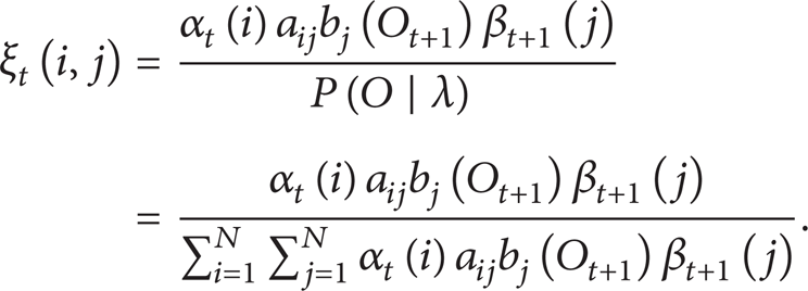
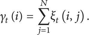
Hence, a probability under state s _i at time t can be defined as

${\gamma }_t\left(i\right)=\sum _{j=\mathrm{1}}^N{\xi }_t\left(i,j\right).$

(5)

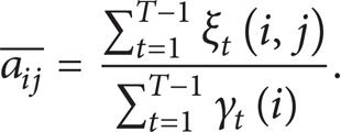
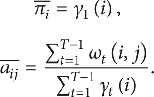
Therefore, the three parameters of HMM model can be estimated. The initial probability distribution can be calculated as

$\stackrel{—}{{\pi }_i}={\gamma }_{\mathrm{1}}\left(i\right).$

(6)

The transition probability distribution can be calculated as

$\stackrel{—}{a_{ij}}=\frac{{\sum }_{t=\mathrm{1}}^{T-\mathrm{1}}{\xi }_t\left(i,j\right)}{{\sum }_{t=\mathrm{1}}^{T-\mathrm{1}}{\gamma }_t\left(i\right)\mathrm{\hspace{0.17em}\hspace{0.17em}}}.$

(7)

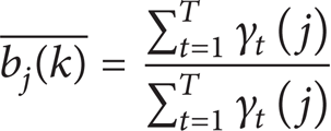
The emission probability distribution can be calculated as

$\stackrel{—}{b_j\left(k\right)}=\frac{{\sum }_{t=\mathrm{1}}^T{\gamma }_t\left(j\right)}{{\sum }_{t=\mathrm{1}}^T{\gamma }_t\left(j\right)}$

(8)

Given an observation sequence O = O₁, O₂, … O _T , Baum-Welch method may be used to estimate λ such that $P(O\mid \lambda )$ is locally maximized. Firstly, three variables are defined as follows.

Forward variable ${\alpha }_t(i)=P(O_{\mathrm{1}},O_{\mathrm{1}},\dots O_t,q_t=S_i\mid \lambda )$ , that is, the probability of the partial observation sequence, O₁, O₂, … O _t , and state S _i at time t, given the model λ.

Backward variable ${\beta }_t(i)=P(O_{t+\mathrm{1}},O_{t+\mathrm{2}},\dots O_T\mid q_t=S_i,\lambda )$ , that is, the probability of the partial observation sequence from t + 1 to the end, given state S _i at time t and model λ.

${\omega }_t(i,j)=P(q_t=S_i,q_{t+\mathrm{1}}=S_j\mid O,\lambda )$ , the probability of being in state S _i at time t, and S _j at time t + 1, given the model λ and the observation sequence O.

The detailed model training steps of MG-HMM are listed as follows.

Step 1. Some variables are firstly defined: state number N, Gaussian mixture component number M, initial state distribution with random initialization, state transition probability distribution A with random initialization and the other parameters needed to construct observation symbol probability distribution in state j with random initialization. Of course the random initialization should be satisfied with the stochastic constraint.

Step 2. Calculate α _t (i). This variable can be solved by dynamic programming algorithm. The solving process is as follows:

$\begin{array}{c}{\alpha }_{\mathrm{1}}\left(i\right)={\pi }_i{b}_i\left(O_{\mathrm{1}}\right),\hspace{1em}\mathrm{1}\le j\le N,\\ {\alpha }_{t+\mathrm{1}}\left(j\right)=\left[\sum _{i=\mathrm{1}}^N{\alpha }_t\left(i\right)a_{ij}\right]b_j\left(O_{t+\mathrm{1}}\right),\\ \hspace{1em}\hspace{1em}\hspace{1em}\hspace{1em}\mathrm{1}\le j\le N,\hspace{1em}\mathrm{1}\le t\le T-\mathrm{1}.\hfill \end{array}$

(9)

Step 3. Calculate β _t (i). The solving process is as follows:

$\begin{array}{c}\begin{array}{c}{\beta }_T\left(i\right)=\mathrm{1},\hspace{1em}\mathrm{1}\le j\le N,\\ {\beta }_t\left(j\right)=\sum _{j=\mathrm{1}}^N{a}_{ij}{b}_j\left(O_{t+\mathrm{1}}\right){\beta }_{t+\mathrm{1}}\left(j\right),\hspace{1em}\mathrm{1}\le j\le N,\\ \hspace{1em}\hspace{1em}\hspace{1em}\hspace{1em}\hspace{1em}\hspace{1em}\hspace{1em}t=T-\mathrm{1},T-\mathrm{2},\dots ,\mathrm{1}.\end{array}\end{array}$

(10)

Step 4. Calculate ${\omega }_t(i,j)=P(q_t=S_i,q_{t+\mathrm{1}}=S_j\mid O,\lambda )$ for each time t:

$\begin{array}{c}{\omega }_t\left(i,j\right)=\frac{{\alpha }_t\left(i\right)a_{ij}{b}_j\left(O_{t+\mathrm{1}}\right){\beta }_{t+\mathrm{1}}\left(j\right)}{P\left(O\mid \lambda \right)}\\ \hfill =\frac{{\alpha }_t\left(i\right)a_{ij}{b}_j\left(O_{t+\mathrm{1}}\right){\beta }_{t+\mathrm{1}}\left(j\right)}{{{\sum }_{i=\mathrm{1}}^N\sum }_{j=\mathrm{1}}^N{\alpha }_t\left(i\right)a_{ij}{b}_j\left(O_{t+\mathrm{1}}\right){\beta }_{t+\mathrm{1}}\left(j\right)}\end{array}$

(11)

Step 5. Calculate γ _t (i) = ∑ _{i = 1} ^N ω _t (i, j) for each time t.

Step 6. Calculate updated initial probability distribution π and state transition probability distribution A:

$\begin{array}{c}\stackrel{—}{{\pi }_i}={\gamma }_{\mathrm{1}}\left(i\right),\\ \stackrel{—}{a_{ij}}=\frac{{\sum }_{t=\mathrm{1}}^{T-\mathrm{1}}{\omega }_t(i,j)}{{\sum }_{t=\mathrm{1}}^{T-\mathrm{1}}{\gamma }_t\left(i\right)}.\end{array}$

(12)

Step 7. For each time t, state j and the kth component probability in mixture Gaussian distribution can be expressed as

${\gamma }_t(j,k)=\left[\frac{{\alpha }_t\left(j\right){\beta }_t\left(j\right)}{{\sum }_{j=\mathrm{1}}^N{\alpha }_t\left(j\right){\beta }_t\left(j\right)}\right]\left[\frac{c_{jk}N(O_t,{\mu }_{jk},U_{jk})}{{\sum }_{m=\mathrm{1}}^M{c}_{jk}N(O_t,{\mu }_{jk},U_{jk})\mathrm{\hspace{0.17em}\hspace{0.17em}}}\right].$

(13)

Step 8. Estimate the parameters in observation probability density function:

$\begin{array}{c}\stackrel{—}{c_{jk}}=\frac{{\sum }_{t=\mathrm{1}}^T{\gamma }_t(j,k)}{{\sum }_{t=\mathrm{1}}^T{\sum }_{k=\mathrm{1}}^M{\gamma }_t(j,k)},\\ \stackrel{—}{{\mu }_{jk}}=\frac{{\sum }_{t=\mathrm{1}}^T{\gamma }_t(j,k)O_t}{{\sum }_{t=\mathrm{1}}^T{\gamma }_t(j,k)},\\ \stackrel{—}{U_{jk}}=\frac{{\sum }_{t=\mathrm{1}}^T{\gamma }_t\left(j,k\right)\left(O_t-{\mu }_{jk}\right){\left(O_t-{\mu }_{jk}\right)}^{\prime }}{{\sum }_{t=\mathrm{1}}^T{\gamma }_t(j,k)}.\end{array}$

(14)

Step 9. The procedure may end or jump to Step 2 according to the given threshold.

The above model training algorithm can only be applied for a single observation sequence. In practical application, in order to obtain a more reliable estimation of parameters, one has to use multiple observation sequences.

For given multiple sequences $O=[O^{(1)},O^{(2)},\dots ,O^{(z)}]$ and each sequence O^(z) = [O₁^(z), O₂^(z), …, O _{T z} ^(z)], the goal of model training is $P(\lambda \mid O)={\max }_{\lambda }{\Pi }_{z=1}^{z}P(O^{(z)}\mid \lambda )$ . We can adaptively modify the above algorithm to confirm with the multiple sequences. First of all, the likelihood $P(O^{(z)}\mid \lambda )={\sum }_{i=\mathrm{1}}^N{\alpha }_T^z(i)$ of each single sequence is calculated. Hence, the reestimation of parameters should consider the contribution weight of each sequence.

3. FS-LSSVR

SVM has been widely used in many areas [20]. Least squares support vector machine (LSSVM) [21] is a least squares version of SVM for classification problems. The solution of LSSVM follows directly from solving a set of linear equations. Furthermore, the support values in LSSVM are proportional to the errors.

3.1. LSSVM

Given a sample set {y _k , x _k }_{k = 1} ^N where x _k ∊ R ⁿ is the kth input features and y _k ∊ R is the kth label, LSSVM can be described as follows [21]:

$\begin{array}{c}\underset{w,b,e}{\min \mathrm{\hspace{0.17em}\hspace{0.17em}}}\hspace{1em}\hspace{1em}\hspace{0.5em}J=\frac{\mathrm{1}}{\mathrm{2}}{w}^{T}w+\frac{\mathrm{1}}{\mathrm{2}}\gamma \sum _{k=\mathrm{1}}^N{e}_k^{\mathrm{2}}\\ \text{subject}\mathrm{\hspace{0.17em}\hspace{0.17em}}\text{to}\hspace{0.5em}{y}_k\left[w^T\varphi \left(x_k\right)+b\right]=\mathrm{1}-e_k,\\ \hspace{1em}\hspace{1em}\hspace{1em}\hspace{1em}\hspace{1em}\hspace{1em}\hspace{1em}\hspace{1em}\hspace{1em}\hspace{1em}\hspace{1em}k=\mathrm{1},\dots ,N.\end{array}$

(15)

The solution to the constrained optimization problem follows from the Lagrangian:

$L\left(w,b,e;\alpha \right)=J(w,b,e)-\sum _{k=\mathrm{1}}^N{\alpha }_k\left\{y_k\mid \left[w^T\varphi \left(x_k\right)+b\right]-\mathrm{1}+e_k\right\}.$

(16)

Here, the variable α _k is Lagrange multiplier. The problems can be solved by the following equation:

$\begin{array}{c}\frac{\partial L}{\partial w}=\mathrm{0}⟶w={\sum }_{k=\mathrm{1}}^N{\alpha }_k{y}_k\varphi \left(x_k\right),\\ \frac{\partial L}{\partial b}=0⟶{\sum }_{k=1}^N{\alpha }_k{y}_k=0,\\ \frac{\partial L}{\partial e_k}=0⟶{\alpha }_k=\gamma e_k,\hspace{1em}k=1,\dots ,N,\\ \frac{\partial L}{\partial {\alpha }_k}=0⟶y_k\left[w^T\varphi \left(x_k\right)+b\right]-1+e_k=0,\\ \hspace{1em}\hspace{1em}\hspace{1em}\hspace{1em}\hspace{1em}\hspace{1em}\hspace{1em}\hspace{1em}k=1,\dots ,N.\end{array}$

(17)

Similar to the standard SVM, the w and ϕ(x _i ) do not need to be solved. A linear KKT system can be established in place of the two order optimization system to eliminate w and e:

$\left[\begin{array}{cc}\mathrm{0}& {\mathrm{1}}_v^T\\ {\mathrm{1}}_v& \Omega +{\gamma }^{-\mathrm{1}}{I}_N\end{array}\right]\left[\begin{array}{c}b\\ \alpha \end{array}\right]=\left[\begin{array}{c}\mathrm{0}\\ Y\end{array}\right].$

(18)

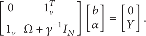
In the above linear equation, there are Y = [y₁; …; y _N ] and 1 _v = [1; …; 1], e = [e₁; …; e _N ], and α = [α₁; …; α _N ]. Meanwhile, according to the Mercer permission condition, the kernel matrix Ω ∊ R^{N × N} can be written as

${\Omega }_{ij}=\varphi {\left(x_i\right)}^T\varphi \left(x_j\right)=K\left(x_i,x_j\right).$

(19)

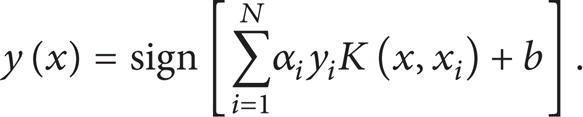
The solution of classification problem is as follows:

$y\left(x\right)=\mathrm{sign}\left[\sum _{i=\mathrm{1}}^N{\alpha }_i{y}_{i}K\left(x,x_i\right)+b\right].$

(20)

3.2. FS-LSSVR

Solving the LS-SVM requires the resolution for all samples, which is practical when the input space dimension is larger than sample size. However, when the sample size is very large, it is impossible to solve these questions by traditional LS-SVM method [22]. For example, the benchmark data set used in Section 5 to finish fault prognostic contains about 200 samples, and the total size is above 20000. For this case, LS-SVR needs to be adjusted to fit for large scale problems. FS-LSSVR is presented to solve this problem [22]. It makes use of the NystrÖm approximation but estimates the model in the primal within the LS-SVM setting [23]. Instead of a random subset, a subset selection method based upon quadratic Renyi entropy was proposed.

1. Nyström Approximation in Dual Space. Nonlinear map φ can be explicitly represented by eigenvalue decomposition of kernel matrix Ω and kernel function K(x, x _j ). For probability density p(x), there is

   $\int K\left(x,x_j\right){\phi }_i\left(x\right)p\left(x\right)dx={\lambda }_i{\phi }_i\left(x_j\right).$

   (21)

   ϕ is represented as follows:

   $\varphi =\left[\sqrt{{\lambda }_{\mathrm{1}}}{\phi }_{\mathrm{1}},\sqrt{{\lambda }_{\mathrm{2}}}{\phi }_{\mathrm{2}},\dots ,\sqrt{{\lambda }_{nh}}{\phi }_{nh}\right].$

   (22)

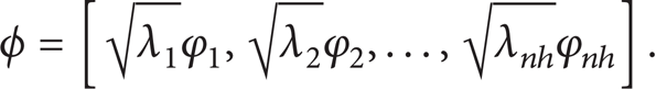
   Here, the φ is eigenvalue function.

   The above problem can be transformed to an eigenvalue problem on the sample data set:

   $\frac{\mathrm{1}}{N}\sum _{k=\mathrm{1}}^{N}K(x_k,x_j)u_i\left(x_k\right)={\lambda }_i^{\left(s\right)}{u}_i\left(x_j\right).$

   (23)

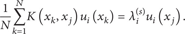
   Then, the eigenvalue λ _i and eigenvalue vector u _i can be approximated by the eigenvalue and eigenvalue vector:

   $\widehat{{\lambda }_i}=\frac{\mathrm{1}}{N}{\lambda }_i^{\left(s\right)},\hspace{1em}\hspace{1em}\widehat{{\phi }_i}=\sqrt{N}{u}_i.$

   (24)

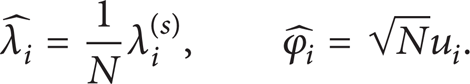
   The nonlinear map is estimated as follows:

   $\widehat{{\varphi }_i}\left(x\right)=\frac{N}{\sqrt{{\lambda }_i^{\left(s\right)}}}\sum _{k=\mathrm{1}}^N{u}_{ki}K\left(x_k,x^{\left(v\right)}\right).$

   (25)

2. Sparse Spproximation for Subset. Small proportion of all samples selected to approximate all samples is the core idea of FS-LSSVR algorithm. The standard of sample selection is of great importance. Entropy maximization is a well-defined criterion for subset selection. Renyi entropy can be considered as one of the criteria:

   $H_R=-\log \int p{\left(x\right)}^{\mathrm{2}}dx.$

   (26)

   It can be approximated as

   $\int \widehat{p}{\left(x\right)}^{2}dx=\frac{\mathrm{1}}{N^{\mathrm{2}}}{\mathbf{1}}^{\mathbf{T}}\mathbf{\Omega }\mathbf{1}.$

   (27)

3. Based on the analysis in (1) and (2), the algorithm can be listed as follows.

Step 1. Randomly select a subset with M samples from the original data set {y _k , x _k }_{k = 1} ^N . The two-order Renyi entropy is calculated for the selected samples. Then, the subset with maximization Renyi entropy is determined.

Step 2. A small kernel matrix Ω _M is constructed based on the selected samples.

Step 3. Compute the eigenvalue λ _i ^(s) and eigenvalue vector u _i on Ω _M .

Step 4. Nonlinear map $\widehat{\varphi }({\text{x}}_{\text{i}})$ is calculated for all samples (i = 1, …, N).

Step 5. The final regression problem is solved based on the above steps.

4. System Framework for RUL Prediction

4.1. LR-HMM

Here LR-HMM model [7] is proposed for RUL prediction as shown in Figure 1.

Figure 1:

LR-HMM Model for RUL prediction.

The health status of system discussed here is S = {1, 2, 3, …, N}. The health status is a oneway and irreversible. From Section 2, we know that the forward variable ${\alpha }_t(i)=P(O_1,O_1,\dots O_t,q_t=S_i\mid \lambda )$ represents the probability of the partial observation sequence, O₁, O₂, … O _t , and state S _i at time t, given the model λ. This definition is used to describe the health status of system. The calculation of α _t (i) is given in (9).

4.2. System Framework

The system is established based on three parts as shown in Figure 2. The first part trains the MG-HMM and FS-LSSVR model. According to the known samples, several MG-HMM models can be trained based on expectation maximization algorithm. Then, the forward variables of each sample can be calculated based on these MG-HMM models. The corresponding FS-LSSVR model is established with these forward variables. The MG-HMM models and corresponding FS-LSSVR models are constructed into a model library. The second part of the system is to recognize the unknown sample based on the model library. This part determines the MG-HMM model and FS-LSSVR with the maximization likelihood.

Figure 2:

System framework.

The third part of the system calculates the forward variables based on the MG-HMM obtained from the second part. These forward variables are put into the corresponding FS-LSSVR model to compute the RUL of the unknown sample.

5. Experiments

5.1. RUL Evaluations Metrics

Fault prognostic has its inherent particularity contrary to fault diagnosis. Therefore, Saxena et al. present some new evaluation metrics on fault prognostics [24–27]. After making a thorough inspection of these metrics, this paper further proposes two metrics for fault prognostics metrics: MAα and α-Nmap. We consider the series of evaluation metrics that could effectively measure algorithm performance in real-time RUL assessment.

First of all, a variable r ^f (t) is defined as the actual RUL when the system is in t moment, while variable r ^p (t) is defined as the prediction RUL at the same time. Hence, the prediction error percentage is represented as

$\text{PE}\left(t\right)=\frac{\left|r^p\left(t\right)-r^f\left(t\right)\right|}{r^f\left(t\right)}.$

(28)

Obviously there is PE ≥ 0. When the PE is equal to zero, there will be a perfect prediction.

(I) MAPE. Assumes the prediction time start that from t = 1 to the final failure moment t = N. Based on the prediction error percentage metrics, there are several evaluation metrics listed below

$\text{MAPE}=\frac{\mathrm{1}}{N}\sum _{t=\mathrm{1}}^N\text{PE}\left(t\right).$

(29)

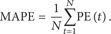
The metrics measure the average prediction precision along with the time axis.

(II) BIAS. Consider the following:

$\text{BIAS}=\sqrt{\frac{\mathrm{1}}{N-\mathrm{1}}\sum _{t=\mathrm{1}}^N\left(\text{PE}\left(t\right)-\text{MAPE}\right)}.$

(30)

The metrics measure the prediction bias along with the time axis.

(III) α(t), α ∊ [0, 1]. If there is [1 – α]r ^f (t) ≤ r ^p (t) ≤ [1 – α]r ^f (t), there will be α(t) = true, otherwise α(t) = false. The metrics gives a Boolean determination whether the prediction time is in a certain earlier or later range away from actual time.

(IV) MAα. Consider the following:

$\text{MA}\alpha =\frac{\mathrm{1}}{N}\left(\sum _{t=\mathrm{1}}^{N}I\left(\alpha \left(t\right)\right)\right),\hspace{1em}\alpha ∊\left[\mathrm{0,1}\right];$

(31)

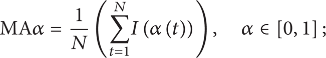
where there is α(t) = true there will be $I(\alpha (t)=\text{true})=\mathrm{1}$ , otherwise, $I(\alpha (t)=\text{true})=\mathrm{0}$ . In fact, these metrics makes a simple statistics of α(t). The great advantage of the metrics is that they do not need to consider specific prediction time point.

(V) α-Nmap. Furthermore, we specify λ = 1/k and α = λm where there is m = {1, 2 …, k}. Hence, the α-Nmap is represented as

$\alpha \text{-Nmap}=\frac{\mathrm{1}}{k}\sum _{m=1}^k\text{MA}\alpha \left(m\lambda \right).$

(32)

The metrics mean the whole prediction correct percentage when the allowable prediction range changes in the interval [anjan101]. Therefore, there is α-Nmap ∊ [0, 1]. Furthermore, the best solution is obtained when α-Nmap = 1.

(VI) C. The metrics indicate the convergence performance of prediction. The detailed description can be provided as follows.

$\begin{array}{c}{x}_c=\frac{\left(\mathrm{1}/\mathrm{2}\right){\sum }_{t=\mathrm{1}}^{N-\mathrm{1}}\left({\left(t+\mathrm{1}\right)}^{\mathrm{2}}-t^{\mathrm{2}}\right)\text{PE}\left(t\right)}{{\sum }_{t=\mathrm{1}}^N\text{PE}\left(t\right)},\\ y_c=\frac{\left(1/2\right){\sum }_{t=\mathrm{1}}^{N-\mathrm{1}}\text{PE}{\left(t\right)}^2}{{\sum }_{t=\mathrm{1}}^N\text{PE}\left(t\right)},\\ C=\sqrt{x_c^2+y_c^2}.\end{array}$

(33)

5.2. Data Set

(C-MAPSS) Commercial modular aeropropulsion system simulation, [24] is a tool for simulating a realistic large commercial turbofan engine. The software simulates an engine model of the 90000 lb thrust class and an atmospheric model capable of simulating operations at (i) altitudes ranging from sea level to 40000 ft, (ii) March numbers from 0 to 0.90, and (iii) sea-level temperatures from −60 to 103°F. Several dataset generated by C-MAPSS has been uploaded on NASA website. The description of the dataset is shown in Table 1.

Table 1:

C-MAPSS data set.

Data Set	Train trajectories	Test trajectories	Conditions	Fault modes
FD001	100	100	One (sea level)	One (HPC Degradation)
FD002	260	259	Six	One (HPC degradation)
FD003	100	100	One	Two (HPC degradation, fan degradation)
FD004	248	249	Six	Two (HPC degradation, fan degradation)

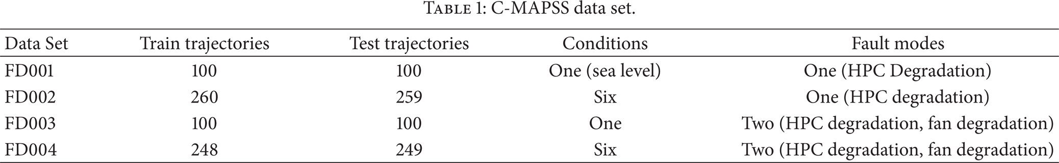
There are 26 columns in these data sets. Column one represents the unit number. Column two is the time of unit running. Columns 3–5 are the different unit operation conditions. The remaining columns are the 21 sensor measurements. The software calculates the health index according to four parameters of the 21 variables. But the researchers could not find these parameters explicitly.

The train trajectories contain all sensor measurements of one unit during its whole life. Otherwise, the test trajectories only provide part of all measurements of one unit. That is, the dataset are truncated at an appropriate time before its failure. The data set is divided into four training sets and four test sets. In the experiments, we used FD001 and FD002 train trajectories as training sets and FD001 and FD002 test trajectories as test set.

In order to train the MG-HMM model on data, we firstly transform the 24 sensor measurements (including 3 columns working conditions and 21 columns other sensor measurements) into values in (0, 1) range by Sigmoid function $x=1/(1+\exp (x))$ . For the considerations of performance and precision, here we choose the HMM model with five states and two Gaussian mixture models. The model training, unknown sample recognition, and RUL prediction process are listed as follows.

1. Four individual MG-HMM models are trained on the four data sets with different work conditions.

2. Health index of different data sets is calculated based on the corresponding MG-HMM.

3. FS-LSSVR models corresponding to the MG-HMM are built based on health index, running cycle t, and RUL of training data set.

4. Online recognition for unknown sample is done based on MG-HMM. In other words, the algorithm determines the unknown sample as the emission of the MG-HMM which has the maximization likelihood on the unknown sample.

5. Health index of the time t is calculated based on the MG-HMM obtained in (4).

6. Based on the time cycle t and health index, the FS-LSSVR corresponding to the MG-HMM obtained in (4) is used to predict the RUL.

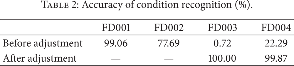
5.3. Condition Recognition

These MG-HMM models are used to judge the work condition of unknown sample. The judgment results are listed in the first row of Table 2. From Table 2, we find the recognition accuracy on FD001 and FD002 is very high, while the recognition accuracy of FD003 and FD002 is very low. The reason is that the FD001 and FD002 only contain one type fault, that is, HPC degradation. However, the FD003 and FD004 contain two type faults; one is HPC degradation and the other is fan degradation. Furthermore, we give a deeper inspector for the dataset. Then we find that FD003 operates under the same condition as FD001 and FD004 operates under the same condition as FD002. Then we adjust the algorithm with respect to the work condition. The algorithm is considered to do right recognition if it judges the FD003 as the emission of MG-HMM1 which is trained from FD001. Similarly, the algorithm is thought to do right recognition if it judges the FD004 as the emission of MG-HMM2 which is trained from FD002. After this adjustment, the accuracy of condition recognition for FD003 is improved from 0.72% to 100%. Meanwhile, the accuracy of condition recognition for FD004 is improved from 22.29% to 99.87%.

Table 2:

Accuracy of condition recognition (%).

	FD001	FD002	FD003	FD004
Before adjustment	99.06	77.69	0.72	22.29
After adjustment	—	—	100.00	99.87

5.4. Health Indexes

We apply the various MG-HMM models obtained from the training data set into health index calculation on the unit 1 of training data set and testing data set. The health indexes are illustrated in Figure 3. In Figure 3, the health state is the first state of MG-HMM and the hazard state is the final state. We find the probability of health decreases as time goes on. Meanwhile, the probability of hazard increases as time goes on. The situation is in line with the actual working condition of the traditional equipment.

Figure 3:

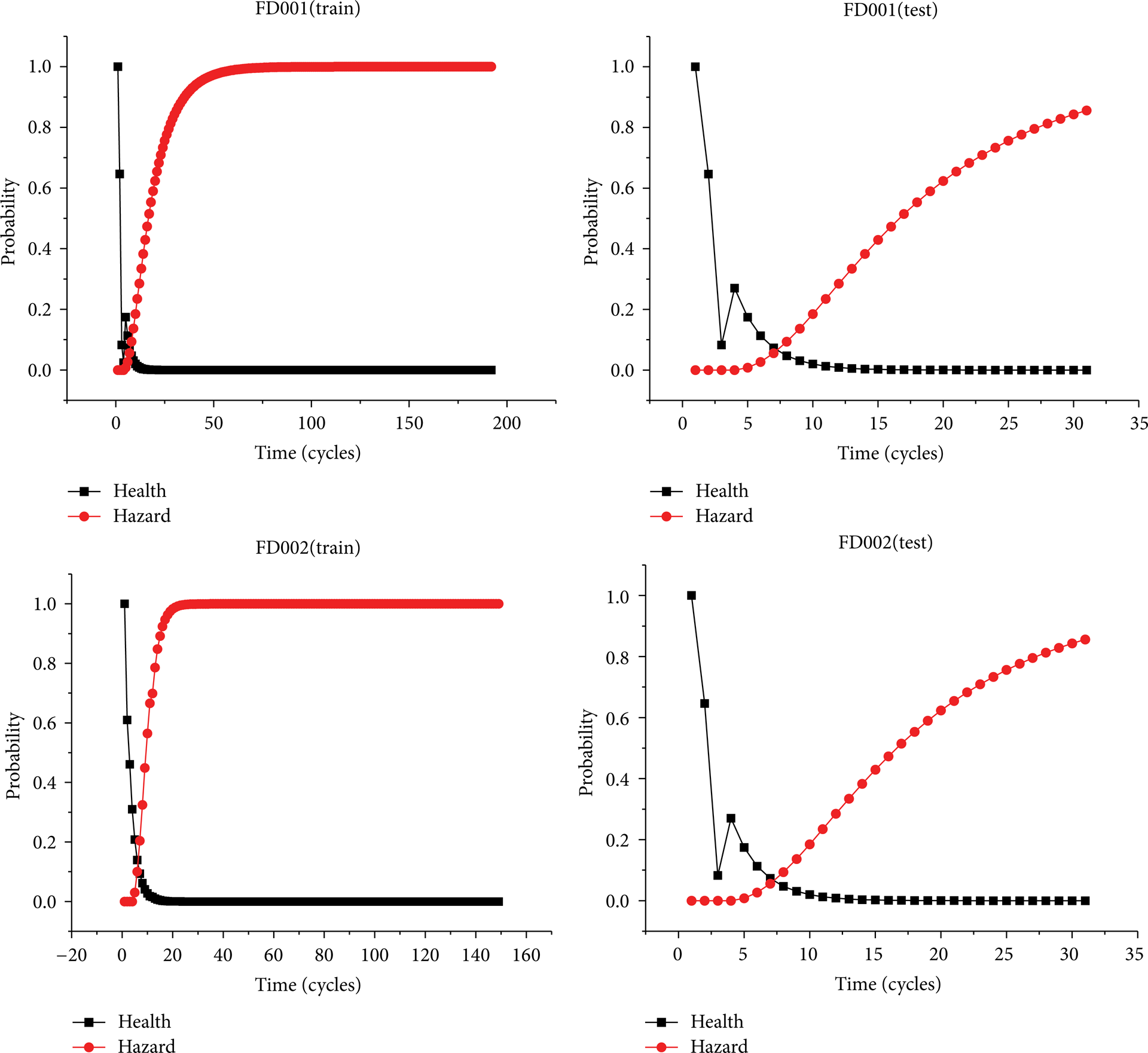
Health indexes for several samples.

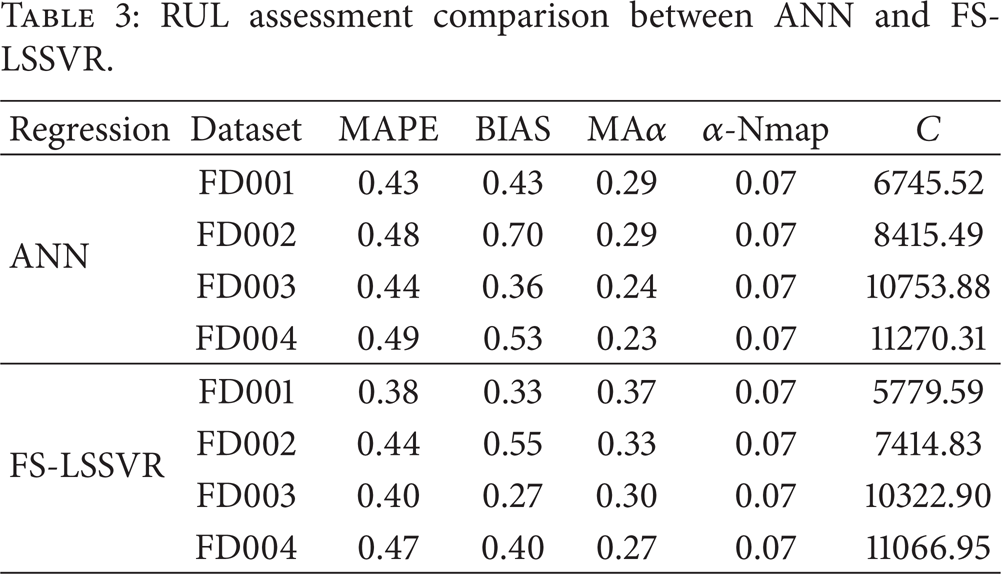
5.5. RUL Assessment

Once health indexes of unknown samples are calculated based on MG-HMM models, the RUL can be predicated based on FS-LSSVR models. Here we also make a comparison between ANN and FS-LSSVR. The reason we choose ANN is that ANN is a good nonlinear regression tool in machine learning area. The comparison results are listed in Table 3. From MAPE metric, we find that the FS-LSSVR can make a higher accuracy RUL prediction than ANN. Based on BIAS metric, we find the deviation of RUL prediction based on FS-LSSVR is lower than ANN. From the comparison result of MAα and α-Nmap, we find the FS-LSSVR can make more near RUL prediction than ANN. Also the FS-LSSVR converges to the failure point faster than ANN.

Table 3:

RUL assessment comparison between ANN and FS-LSSVR.

Regression	Dataset	MAPE	BIAS	MAα	α-Nmap	C
ANN	FD001	0.43	0.43	0.29	0.07	6745.52
	FD002	0.48	0.70	0.29	0.07	8415.49
	FD003	0.44	0.36	0.24	0.07	10753.88
	FD004	0.49	0.53	0.23	0.07	11270.31
FS-LSSVR	FD001	0.38	0.33	0.37	0.07	5779.59
	FD002	0.44	0.55	0.33	0.07	7414.83
	FD003	0.40	0.27	0.30	0.07	10322.90
	FD004	0.47	0.40	0.27	0.07	11066.95

6. Conclusions

In this paper we present a hybrid method of MG-HMM and the FS-LSSVR for fault prognostic. The system contains three parts. The first part is responsible for training the MG-HMM models and FS-LSSVR models. The second part of the system recognizes the unknown sample based on the model library established in the first part. The third part of the system calculates the forward variables based on the MG-HMM obtained from the second part. These forward variables are inputted into the corresponding FS-LSSVR model to compute the RUL of the unknown sample.

Furthermore, after making a thorough inspection for former metrics of RUL assessment, this paper proposes two novel metrics for fault prognostics metrics: MAα and α-Nmap. From the comparison result of MAα and α-Nmap, we find the FS-LSSVR can make more near RUL prediction than ANN.

One interesting direction for future work is to investigate other state judgment techniques. The techniques can be developed based on pattern recognition techniques. Among these techniques the methods which can generate probability of health type are more preferred.

Another interesting direction for future work is to explore different regression methods. For example, the deep neural network (DNN) [25] and extreme learning machine (ELM) [28] are two newly developing machine learning algorithms. Maybe there is a better RUL prediction accuracy if the system framework can replace the FS-LSSVR with DNN or ELM. However, the calculation performance for large scale application of the two algorithms is still open issue, as we have considered in this paper.