
Abstract
Isogeometric analysis (IGA) has been a fundamental step forward in the computational mechanics for the past few years, which maintains the accuracy of the description of computational domain geometry throughout the analysis process. However, the research on IGA in the area of flexible multibody dynamics is little and mainly concentrates on the univariate or bivariate NURBS geometry. This paper applies the trivariate IGA to the flexible multibody dynamics and proposes a continuum mechanics-based method to construct the system dynamic equations within the framework of IGA. A significant feature of this method is that it only employs the position coordinates of the control points as the system variables. To solve the large rotation and deformation coupled problems without introducing any rotation angles, the Green-Lagrange strain tensor is adopted. The evaluation of the elastic force and its Jacobian is easy and accurate by exploiting the appropriate mathematical transformation. In addition, the mass matrix and the generalized gravity force remain constant, and the centrifugal and Coriolis inertia forces equal zero. A numerical experiment is conducted using a thin-plate pendulum, which proves the feasibility and effectiveness of this method.
1. Introduction
The kinematic description of flexible bodies that undergo large rotation and deformation is a research hotspot in the area of flexible multibody dynamics. Various methods have been proposed over the years [1], among which the floating frame of reference (FFRF) is the most widely used way. FFRF uses two sets of coordinates to describe the configuration of the deformable bodies; one set describes the position and orientation of a body-fixed coordinate system, and the other describes the deformation of the body with respect to its body-fixed coordinate system. As a consequence, the stiffness matrix used to obtain elastic forces remains the same. However, the mass matrix, centrifugal and Coriolis inertia forces, and generalized gravity forces are highly nonlinear. Moreover, the small deformation assumption limits the use of FFRF in large deformation problems.
In order to overcome the limitation of FFRF, the incremental finite-element approach introduces infinitesimal rotation angles as nodal variables. However, this approach cannot exactly describe the rigid-body motion, which is a fundamental requirement in flexible multibody dynamics.
To solve the drawback of the incremental finite-element approach, the large rotation vector formulation replaces the infinitesimal rotation angles with finite ones. However, this method has not been widely accepted due to the redundancy of representing the large rotation of the cross-section which may lead to singularity problems and unrealistic shear forces.
Absolute nodal coordinate formulation (ANCF) introduces absolute displacements and global slopes as nodal coordinates, which prevents the system equations from being highly nonlinear because the mass matrix and generalized force remain constant and centrifugal and Coriolis inertia forces equal zero. ANCF can exactly describe the rigid body modes and solve the large rotation and deformation problems, while FFRF is just effective in small deformation situations.
Different from the above methods, isogeometric analysis (IGA) [2, 3], which has been considered as a fundamental step forward in computational mechanics, aims to maintain the same exact description of the computational domain geometry throughout the analysis process. The basic idea is the use of the same NURBS-based mathematical model, which is the predominant technology used by CAD, for both modeling and FEA analysis. This makes it possible to exactly represent certain geometries that can only be approximated by polynomial functions, such as conic and circular sections. Moreover, it uses the shape functions with higher regularity than the traditional FEM. IGA exhibits many advantages and has been successfully applied in many problems, for example, contact problems [4], optimization problems [5], shell and plate problems [6–10], fluid-structure interaction problems [11], and so on. In flexible multibody dynamics, [12, 13] compare IGA and ANCF. Reference [14] analyzes the Kirchhoff-Love shells within the framework of IGA. However, most of the prior research uses the univariate or bivariate NURBS geometries to describe the deformable bodies. This paper applies the trivariate IGA to flexible multibody dynamics and proposes a continuum mechanics-based systematic method to solve the large rotation and deformation coupled problems.
The rest of the paper is organized as follows. Section 2 makes a short review of the geometric modeling and computational domain discretization techniques used in IGA. Section 3 proposes a systematic method to construct the dynamic models within the framework of IGA. Section 4 describes the computational strategies used to solve the system equations. To verify the feasibility and effect of this method, numerical tests are performed and the results are presented in Section 5. A conclusion is made at last in Section 6.
2. Geometric Modeling and Space Discretization
IGA forms the computational domain in a way much the same as that of the traditional FEMs. In these methods, the position of any point in an element is evaluated by interpolation of element nodes, and the interpolation weights are determined by the element shape functions. IGA employs NURBS as the geometric description method which is based on the knot vectors, and control points. Meshing and element shape functions are formed by knot vectors and the control points play the same role as that of the element nodes.
A knot vector, Ω = {ξ1, ξ2, …, ξn + p + 1}, is constituted by nondecreasing real numbers, where p is the order of the B-Spline and n is the number of basis functions (and control points) necessary to describe it. A knot vector is said to be uniform if its knots are uniformly spaced and nonuniform otherwise. Moreover, a knot vector is said to be open if its first and last knots are repeated p + 1 times. In this paper, the open knot vectors are adopted. In addition, ξ1 and ξn + p + 1 are set to 0 and 1, respectively.
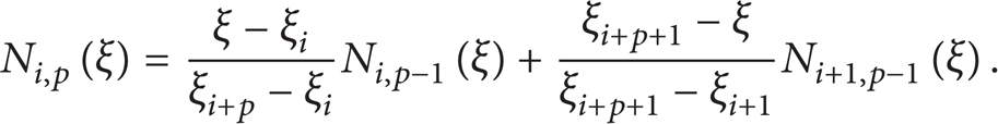
Given a knot vector, Ω, B-Spline basis functions are defined recursively starting with p = 0 (piecewise constants) as follows:
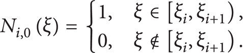
For p > 1,
If the internal knots are not repeated, B-Spline basis functions are Cp−1-continuous. If a knot has multiplicity k, the basis is Cp–k-continuous at that knot. In particular, when a knot has multiplicity p, the basis is C0-continuous and interpolatory at that location.
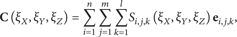
With the knot vectors and the control points, NURBS can form curves, surfaces, and solids exactly. In this paper, we concentrate on the trivariate NURBS solid, on which any point
where ξ
X
, ξ
Y
, and ξ
Z
are the three parameters located in the knot vectors Ω
X
, Ω
Y
, and Ω
Z
, respectively;
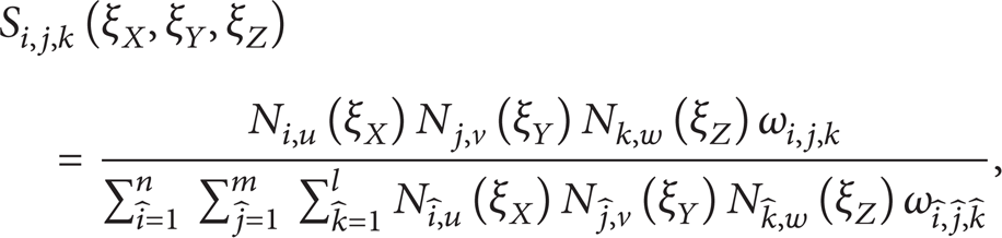
where ωi, j, k are weights; {Ni, u (ξ X )}, Nj, v (ξ Y ), and Nk, w (ξ Z ) are the B-Spline basis functions defined on the knot vectors Ω X , Ω Y , and Ω Z , respectively. It can be easily deduced that the number of NURBS basis functions is N e = n × m × l.
The most distinguished feature of IGA is the discretization of the computational domain. To directly perform the meshing on the same exact NURBS geometry, knot vectors
3. Dynamic Equations
The large rotation and deformation problems of the flexible bodies belong to the highly nonlinear problems. To extend IGA to these problems, a continuum mechanics-based method is proposed to describe the elastic forces.
Suppose that the position vector
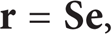
where
where

where
Given the initial configuration

To solve the large rotation and deformation problems within the framework of IGA, the Green-Lagrange strain tensor and the corresponding second Piola-Kirchhoff stress tensor are employed to guarantee that the work of elastic forces and strain energy are not affected when the continuum undergoes pure rigid-body motion.
The Green-Lagrange strain tensor is defined as

With this strain tensor, the weak form of dynamic equilibrium equations of the continuous body in the reference configuration can be written as

The first integral in (10) represents the virtual work of inertia forces, where ρ is the density of material,
3.1. Inertia Forces
The virtual work of inertia forces can be written as

It can be inferred from (11) that the vector of inertia forces is

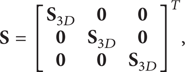
and the mass matrix is
It can be deduced that the mass matrix
3.2. Elastic Forces
As shown in (10), the Green-Lagrange strain tensor is used to measure the degree of deformation in this paper. In order to deduce the expression of the elastic forces, the detailed formula of the Green-Lagrange strain tensor is needed. Suppose

Substituting (14) into (8), the position vector gradients can be written as

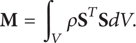
Substituting (15) into (9), the elements of the Green-Lagrange strain tensor can be written as
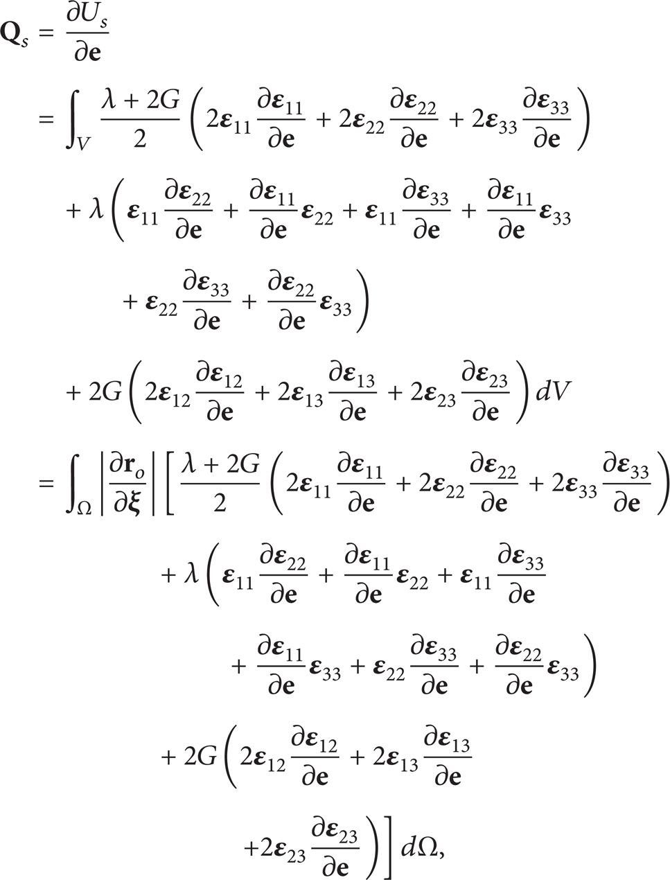
For isotropic elastic materials, the virtual work of elastic forces, U s , can be written as

where λ is Lame's constant and G is the shear modulus. The vector of elastic forces is defined as the derivative of U
s
with respect to generalized coordinates
where

It can be seen from (14), (16), (18), and (19) that

With (18) and (20), the elastic forces and the Jacobian can be effectively evaluated. In engineering problems, mechanical properties of isotropic elastic materials are usually given in terms of Young's modulus, E Y , and Poisson's ratio, μ. The relationships between these parameters and Lame's constants are the following:

3.3. Body Forces
Taking gravity forces as an example, the virtual work of body forces can be written as

It can be inferred that the vector of gravity forces is

4. Computational Strategies
Multibody systems usually contain various forms of constraints. Different kinds of system equations for the constrained multibody systems have been proposed over the years [17, 18]. This paper adopts the frequently used DAE system of index-3 with holonomic constraints which is usually written as
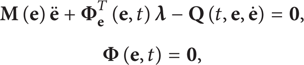
where
In general, DAE-solvers can be classified into two categories [17, 18]: algebraic elimination and constraint violation stabilization. The latter is paid continuously increasing attention due to the simplicity and efficiency in implementation, among which the commonly used methods include Newmark [19], BDF [20], HHT [21], generalized-α [22, 23]. The Newmark method has only order-1 convergence of errors, while the others possess order-2 convergence. In addition, the generalized-α method has adjustable control of numerical dissipation; which leads to an optimal combination of high-frequency and low-frequency dissipation, that is, for a desired level of high-frequency dissipation, the low-frequency dissipation is minimized. Based on these considerations, the generalized-α method is employed to solve the system equation (24). With this method, system equations of time step n + 1 are discretized as

where h is the time step, α m = (2ρ∞ – 1)/(ρ∞ + 1), α f = (ρ∞)/(ρ∞ + 1), ρ∞ ∊ [0, 1], and β = (1 + α f – α m )2/4. ρ∞ is a parameter controlling numerical dissipation (ρ∞ = 0 for maximal dissipation). The position and velocity variables of time step n + 1 are discretized as

where γ = 1/2 + α
f
– α
m
;

Algorithm 1 sums the process of generalized-α scheme to solve dynamic equilibrium at time tn + 1.

Generalized-α scheme.
The Jacobian,

5. Numerical Tests
In this section, a numerical experiment with a thin-plate pendulum is performed to verify the proposed continuum mechanics-based trivariate isogeometric analysis for the large rotation and deformation coupled problems.
As shown in Figure 1, the plate is fixed in one corner without any deformation at the initial time. Then, it falls down freely under the action of gravity. Both the length and width of the plate are set to 3 m, and its thickness is chosen to be 0.1 m. The density, Young's modulus, and Poisson ratio of the material are assumed to be 5000 kg/cm3, 1. 0 × 107 N/m2, and 0.3, respectively.

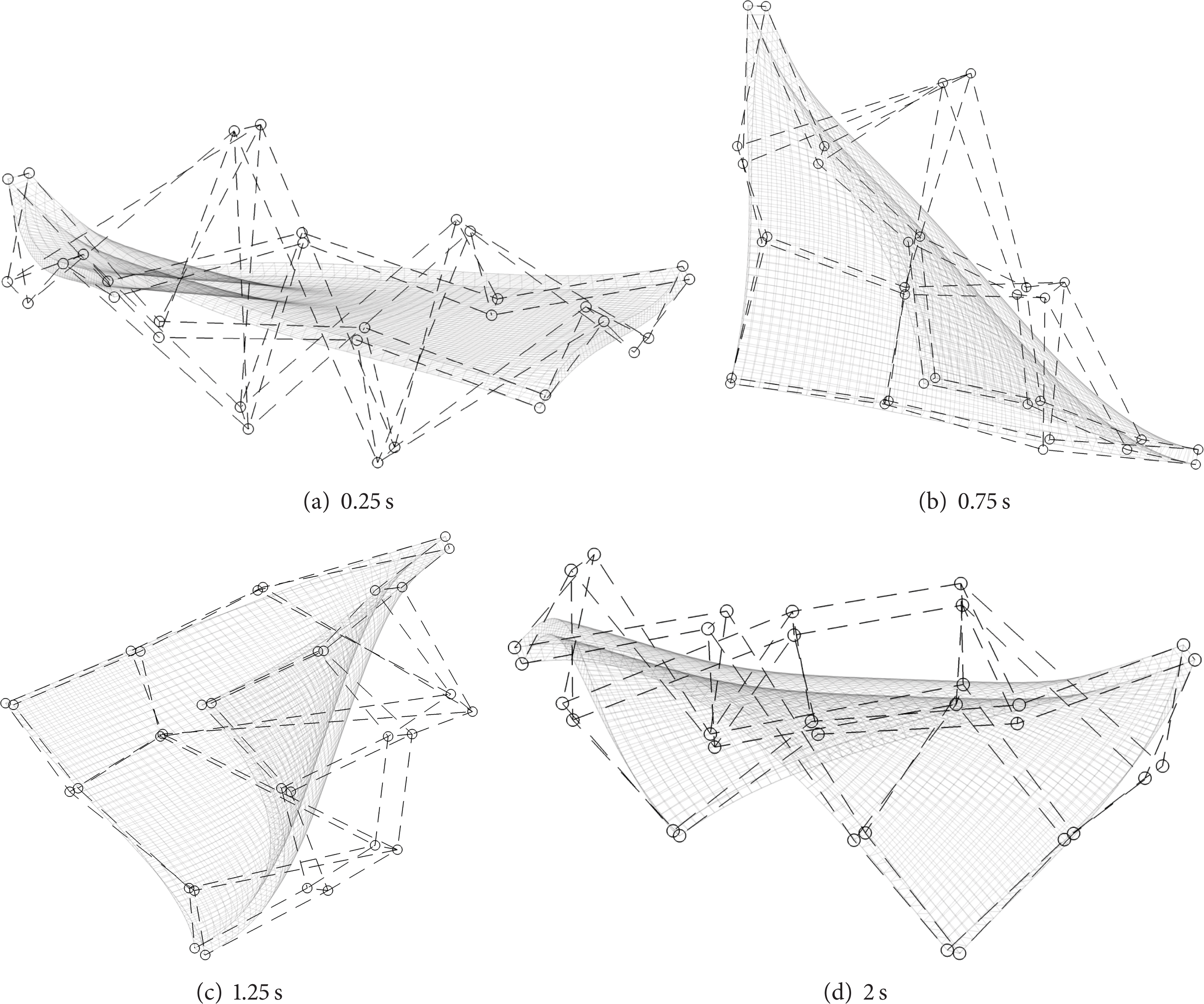
The configuration of the thin plate at different moments (36 elements).
The employed plate element adopts NURBS bases of order 3 in the direction of both length and width. In order not to make a distraction, these NURBS bases are assumed to be C2-continuous at all of the internal knot values, which are uniformly distributed between 0 and 1. The polynomial order in the thickness direction is chosen to be 1. Therefore, the number of control points in a single element is 4 × 4 × 2 = 32.
To better illustrate the NURBS element, Figure 2 presents the relationship between the element and its related control points when the whole plate is regarded as a single element, that is, Ω x = Ω y = {0, 0, 0, 0, 1, 1, 1, 1}, and Ω z = {0, 0, 1, 1}. As shown in the figure, control points are marked with circles and connected with dashed line to form the control net. It should be noted that this is a special case that NURBS basis functions are interpolatory at all of the corners of the element. In most cases, control points do not need to lie on the geometry.

Relationship between the element and the corresponding control points.
To see the influence of refinement on the plate's deformation, other 36-elements (Ω x = Ω y = {0, 0, 0, 0, 1/6, 1/3, 1/2, 2/3, 5/6, 1, 1, 1, 1}, Ω z = {0, 0, 1, 1}) and 100-element (Ω x = Ω y = {0, 0, 0, 0, 0.1, 0.2, 0.3, 0.4, 0.5, 0.6, 0.7, 0.8, 0.9, 1, 1, 1, 1}, Ω z = {0, 0, 1, 1}) meshing plans are performed separately. A 2 s simulation with 2−12 s step size is performed for each of the above three meshing plans. Figure 1 shows the configurations of the moving thin plate at different moments for the 36-element meshing plan. Figure 3 shows the position relationship between the control points and the thin plate configuration for the single-element meshing plan at different moments. Figure 4 compares the plate deformation of single-element, 36-element and 100-element meshing plans at different moments. It is obvious that the plate configuration changes significantly when the number of elements increases from 1 to 36, while it differs not that much from 36 to 100. But the ratio of CPU time used in the three cases is 1: 22: 66. Therefore, it can be concluded that, using this method, a balance between the accuracy and efficiency can be achieved with a relatively coarse meshing.
The configuration of the plate and related control points at different moments (1 element).
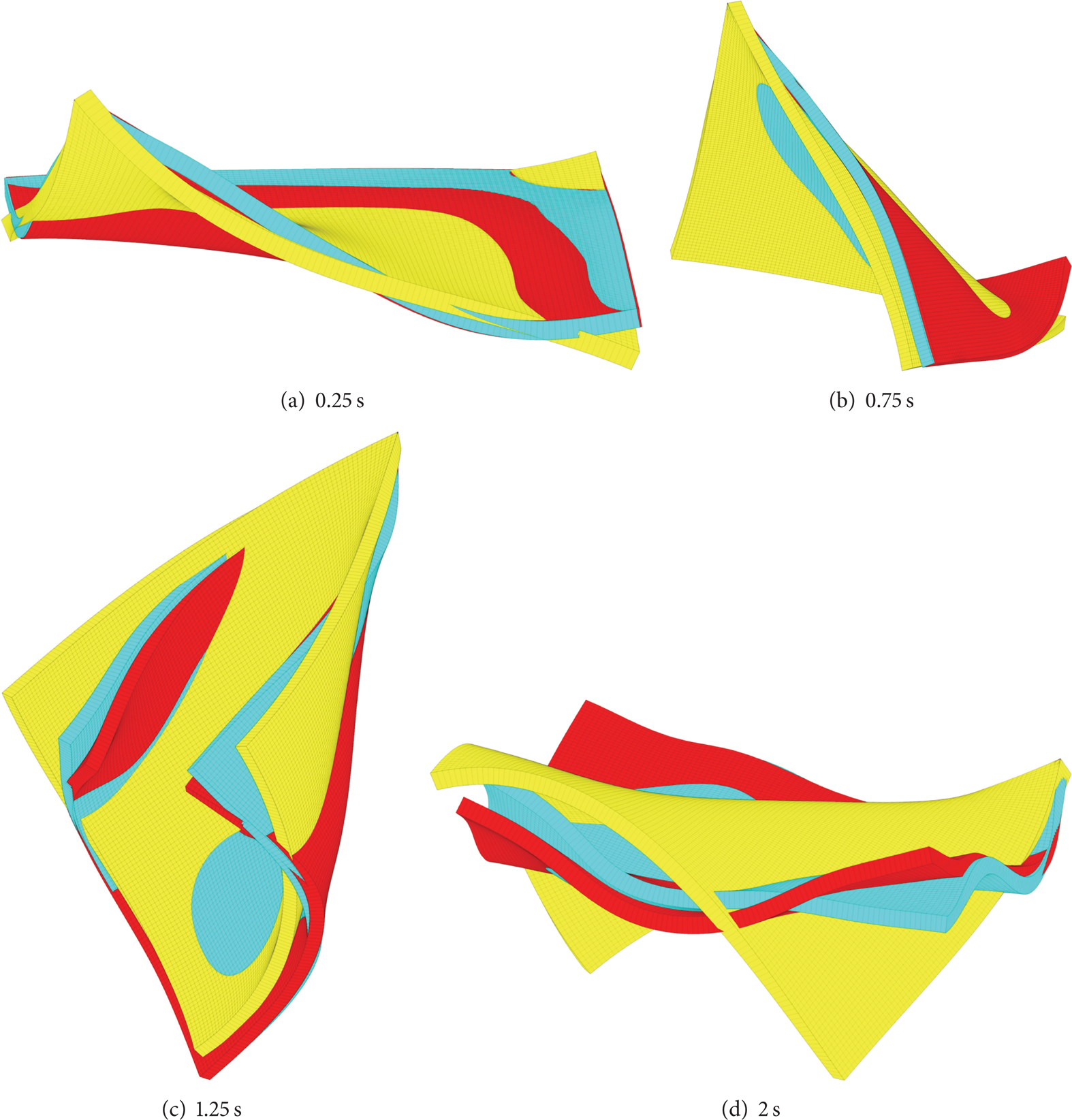
Comparison of plate deformation of different meshing plans (1 element: yellow; 36 elements: cyan; 100 elements: red).
6. Conclusion
This paper applies the trivariate IGA to the flexible multibody system dynamics and proposes a continuum mechanics-based method to construct the system dynamic equations within the framework of IGA. A significant feature of this method is that it only employs the position coordinates of the control points as the system variables. To solve the large rotation and deformation coupled problems without introducing any rotation angles, the Green-Lagrange strain tensor is employed. Elastic force and its Jacobian are easily and accurately evaluated by using appropriate mathematical transformations. In addition, the mass matrix and generalized gravity force remain constant, and the centrifugal and Coriolis inertia forces equal zero. The feasibility and effectiveness of this method are verified through a thin-plate pendulum experiment. In addition, the trivariate IGA has a good symmetric form, which facilitates the computer implementation. The element types and the comparison with other methods will be studied in the future.