Sage Journals: Discover world-class research

Abstract

A numerical method is proposed to compute full-tensor permeability of porous media without artificial simplification. Navier-Stokes (N-S) equation and Darcy's law are combined to design these numerical experiments. This method can successfully detect the permeability values in principle directions of the porous media and the anisotropic degrees. It is found that the same configuration of porous media may possess isotropic features at lower Reynolds numbers while manifesting anisotropic features at higher Reynolds numbers due to the nonlinearity from convection. Anisotropy becomes pronounced especially when convection is dominant.

1. Introduction

Permeability is a key parameter of porous media because it relates with many parameters, such as the infiltration, dielectric strength and thermophysics. It may strongly affect the design and production process of fibrous reinforcements, cement paste and so forth and related scientific researches. The permeability may vary over several orders of magnitude, and it plays an important role in petroleum migration and reservoir performance [1]. Therefore, the accurate measurement of permeability is always a hot topic in both industrial and academic fields. Many of these researches adopt experimental approaches, such as free-space methods, open-ended coaxial probe techniques, cavity resonators, transmission-line techniques, and gas-dynamic methods [2, 3].

Jensen and Heriot-Watt [4] proposed a statistical model for small-scale permeability using minipermeameter and core plug measurements. They suggested the minipermeameter measurement as a better choice. Wang et al. [5] discussed two experimental methods to determine the absolute values of in-plane permeability. They concluded that both the radial flow measurement method and the unidirectional flow measurement method were recommended to obtain reliable permeability data. Ferland et al. [6] proposed a concurrent method to estimate permeability at low cost. However, the experimental procedures can introduce uncertainty significantly on the estimated permeability. They suggested some special treatments to increase the reliability of experimental data. Some other researchers [7 –10] also realized that permeability is difficult to measure although its definition is simple. Many factors, such as flow rate, pressure, fluid properties, handling process by human factors, edge effect, wall effect, single-equipment reproducibility, and between-equipment repeatability, could strongly influence the results of measurements. Therefore, the ability to obtain consistent permeability data depends on skilled and experienced experimental design, reproducible preparation of specimens, operation of equipment, and evaluation of measured raw data. This is the reason many published data observed by different persons often have significant differences for the same material. Weitzenböck et al. [11] pointed out that numerous practical problems caused three-dimensional (3D) permeability measurements to be very difficult. Then, they proposed an approach to measure the permeability by a two-dimensional (2D) radial flow method, which allows the experimental axes not to align with the principal direction of permeability [12, 13].

Some researchers made efforts on measuring transport properties (including permeability) by numerical simulation. Keehm et al. obtained good results in estimating permeability and electric conductivity of complicated pore geometries using Lattice-Boltzmann method (LBM) [14]. Kameda et al. applied LBM to estimate 3D permeability through 2D images of small fragments of rocks. They obtained a valid permeability-porosity trend by using a significant number of such small fragments in statistical sense [15]. Saenger et al. estimated permeability through LBM flow simulation and compared mechanical and transport properties for the same digital rocks [16].

Since all physical parameters can be easily and exactly controlled in numerical simulations, the shortcomings of laboratory experiments mentioned previously can be avoided. In particular, numerical methods have the advantage of separately studying different physical processes coexisting in nature, which are uneasily separated in laboratory. It is easier to form standardization of measurement methods and obtain unchangeable results. It will be a very efficient and economical way for measuring properties of porous media combining with the digital rock physics [17, 18]. In the present paper, we studied how to establish this digital laboratory method for measuring permeability of porous media through directly solving the N-S equation, other than reconstructing it by LBM method. To the best knowledge of the authors, all studies of permeability prediction have been concerned only with diagonal permeability tensor actually. Full tensor of permeability has not been studied extensively since it has more general meanings for practical applications. Thus, we expand our research object from the simple diagonal permeability tensor to more general full permeability tensor. We select gravity in periodic domain as the driven force, instead of pressure widely used in previous studies [1 –18]. This can avoid the edge effect encountered in experimental measurements. As a first trial, we assume incompressible single-phase flow to pass through the porous media in rectangular geometry, but the methodology can be extended to more complex applications, for example two-phase flow using diffuse interface models, which will be pursued in our future researches. The basic principles and proposed methods in this study will be presented next.

2. Principles and Methods

2.1. General Principles

The basic law that is used by experimental and numerical studies for measuring permeability is the Darcy's law:

u_{D} = - \frac{k}{μ} (\nabla p - ρ g),

(1)

where u_D is Darcy velocity (m/s), k is the permeability tensor (m²), g is the gravitational acceleration (m/s²), ∇ p is the pressure gradient (Pa/m), ρ is the density of fluid (kg/m³), and μ is the dynamic viscosity of fluid (Pa · s).

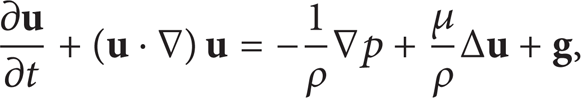
The N-S equation (2) and the continuity equation (3) that describe fluid flow in the continuum sense are as follows (Δ is the Laplace operator):

\frac{\partial u}{\partial t} + (u \cdot \nabla) u = - \frac{1}{ρ} \nabla p + \frac{μ}{ρ} Δ u + g,

(2)

\nabla \cdot u = 0 .

(3)

Conventional methods for measuring permeability neglect gravity and drive the fluid flow by pressure because it is easier to control, especially for laboratory experiments. Here, we select to use the full expressions of (1)∼(3) to determine the permeability. Periodic boundary condition is adopted so that boundary pressure needs not to be considered. It is pretty easier for numerical implementation and more sensible in nature because subsurface formation is in fact a periodic system or statistically periodic one. The general procedure is stated below.

Step 1. Solve (2) and (3) for incompressible single-phase flow in porous media and obtain several velocity fields as samples.

Step 2. Obtain volumetric velocity of the whole domain according to the samples obtained in Step 1.

Step 3. Solve permeability for the whole domain by directly setting the volumetric velocity as the Darcy velocity in (1).

The detailed numerical methods used in these three steps will be introduced in the next section.

2.2. Numerical Methods

As stated previously, we only consider simple 2D rectangular cases in the present study. The incompressible single-phase flow in porous media is modeled as the flow passing through a square barrier in a square domain with periodic boundary conditions. The numerical model is shown in Figure 1(a). L is the domain side length while a is the side length of the barrier. Γ_P means periodic boundary.

Figure 1:

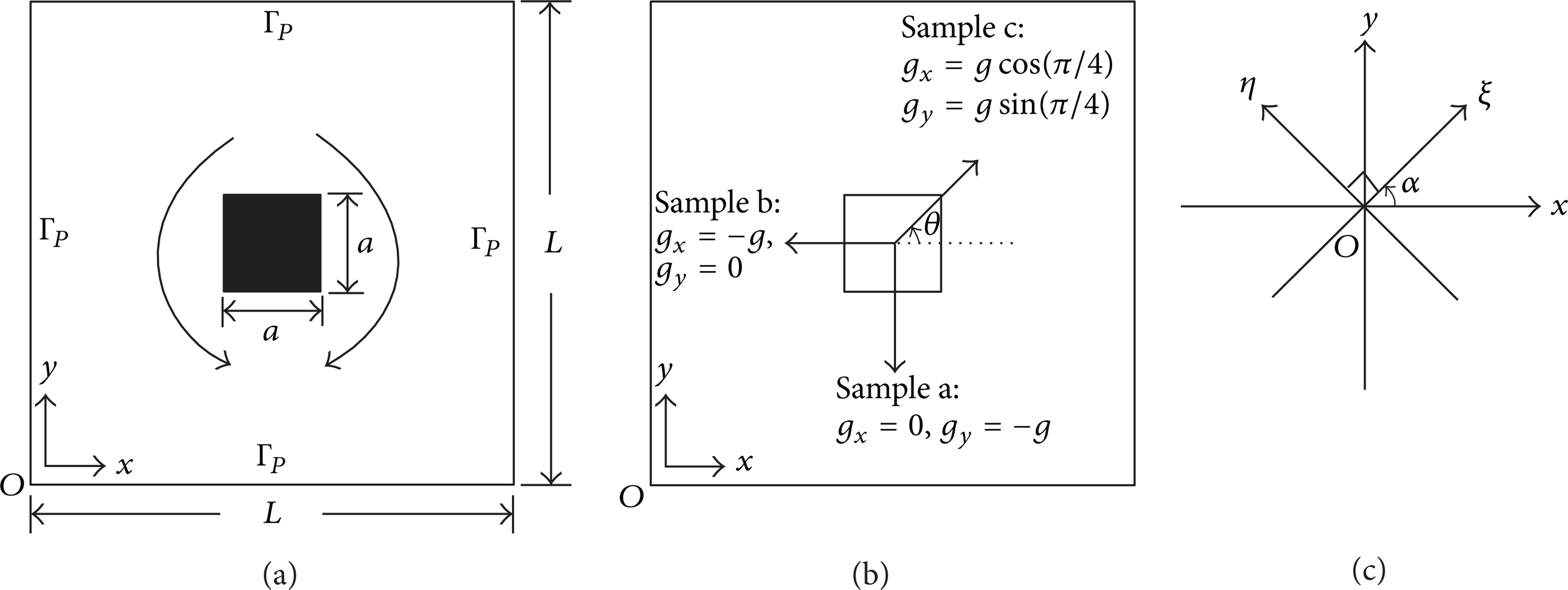
Calculation methodology: (a) numerical model; (b) sampling; and (c) coordinate rotation.

On this kind of domain, the vectors and tensors in (1)∼(3) have the following forms:

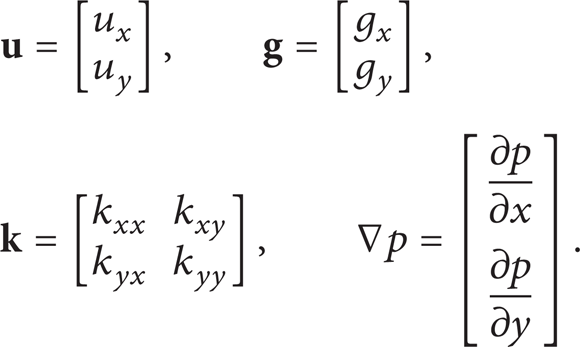
\begin{matrix} u = [\begin{bmatrix} u_{x} \\ u_{y} \end{bmatrix}], g = [\begin{bmatrix} g_{x} \\ g_{y} \end{bmatrix}], k = [\begin{bmatrix} k_{x x} & k_{x y} \\ k_{y x} & k_{y y} \end{bmatrix}], \nabla p = [\begin{bmatrix} \frac{\partial p}{\partial x} \\ \frac{\partial p}{\partial y} \end{bmatrix} \end{matrix}

(4)

Here g_x = gcosθ, g_y = gsinθ, g = 9.807 m/s², k_xx, and k_yy are the diagonal components of the permeability tensor while k_xy and k_yx are the off-diagonal components of the permeability tensor. These four variables are all independent of each other. Three typical directions of gravity are chosen to calculate the full-tensor permeability. They are represented by θ = 3π/2,π, and π/4, respectively, and named “Sample a,” and “Sample b,” and “Sample c” as shown in Figure 1(b).

The numerical algorithm for solving (2)∼(3) in “Step 1” is projection method with fully explicit spatial discretization (but solve pressure implicitly) using second-order finite difference central type scheme. Cyclic tridiagonal matrix algorithm (CTDMA) is applied to accelerate the convergence of pressure iteration. The mesh size is set as 80 × 80. Flow is considered to reach the steady state as the temporal truncation | ∂u/∂t| averaged over the whole domain is lower than 10⁻⁶ m/s².

The volumetric velocity in “Step 2” is defined as follows:

U = \frac{1}{V_{d}} \int_{V_{d}} u d V_{d},

(5)

where $U = [\begin{smallmatrix} U_{x} \\ U_{y} \end{smallmatrix}]$ is the volumetric velocity with the components U_x and U_y in the x and y directions. V_d is the volume of the whole domain. Equation (5) has a discrete expression in this study:

U_{x} = \frac{(\sum u_{x})}{N_{x}}, U_{y} = \frac{(\sum u_{y})}{N_{y}},

(6)

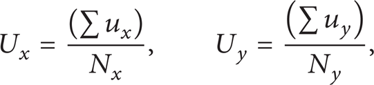
where N_x and N_y are the total number of u_x and u_y on grid cells, respectively. The values of u_x and u_y can be determined by solving the N-S equation so that U_x and U_y can be determined.

The volumetric velocity in (5) is actually the Darcy velocity in (1); that is, u_D = U. In the Darcy scale averaged in the whole domain, pressure gradient should be zero because of the periodic boundary condition; that is, ∇ p = 0. Thus, (1) can be rewritten as

U = \frac{k}{μ} ρ g .

(7)

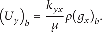
For Sample a ((g_y)_a = – g), (7) becomes

{(U_{x})}_{a} = \frac{k_{x y}}{μ} ρ {(g_{y})}_{a},

(8a)

{(U_{y})}_{a} = \frac{k_{y y}}{μ} ρ {(g_{y})}_{a} .

(8b)

For Sample b ((g_x)_b = – g), (7) becomes

{(U_{x})}_{b} = \frac{k_{x x}}{μ} ρ {(g_{x})}_{b},

(9a)

{(U_{y})}_{b} = \frac{k_{y x}}{μ} ρ {(g_{x})}_{b} .

(9b)

For Sample c ((g_x)_c = gcos(π/4), (g_y)_c = gsin(π/4)), (7) becomes

{(U_{x})}_{c} = \frac{k_{x x}}{μ} ρ {(g_{x})}_{c} + \frac{k_{x y}}{μ} ρ {(g_{y})}_{c},

(10a)

{(U_{y})}_{c} = \frac{k_{y x}}{μ} ρ {(g_{x})}_{c} + \frac{k_{y y}}{μ} ρ {(g_{y})}_{c} .

(10b)

Theoretically, (8a), (8b), (9a), and (9b) are adequate to determine the four components of the full-tensor permeability. However, (U_x)_a and (U_y)_b are always very close to zeros since they are orthogonal to the bulk flow directions and large numerical errors may exist. Thus, k_xy and k_yx determined by (8a) and (9b) are always very close to zeros. This apparently violates the fact that k_xy and k_yx may be far from zeros for some cases. The application of (8a) and (9b) actually makes the full-tensor permeability decay to a diagonal permeability so that they should be canceled. To predict the off-diagonal components accurately, (10a) and (10b) are utilized since the bulk flow in Sample c has equivalent projections in the x and y directions so that (U_x)_c and (U_y)_c are both accurate. Therefore, the final equations to determine the four components of the permeability tensor should be the four equations (8b), (9a), (10a), and (10b), which are used in “Step 3.” The procedure is calculating k_xx by (9a) and k_yy by (8b) and substituting them to (10a) and (10b) to obtain k_xy and k_yx, respectively.

In practice, it is of interest to detect the maximum permeability, the minimum permeability, principle direction, and anisotropy so that essential features of reservoir, which are independent of coordinate systems and samplings, can be described. Therefore, the original permeability tensor can be transformed by rotating the original xOy coordinate to a new ξOη coordinate according to tensors' characteristics [19]. The angle between the ξOη coordinate system and the xOy coordinate system is represented by the angle α (Figure 1(c)). Therefore, a series of transformed permeability tensors $k_{trans} = [\begin{smallmatrix} k_{ξ ξ} & k_{ξ η} \\ k_{η ξ} & k_{η η} \end{smallmatrix}]$ can be obtained by continuously rotating the ξOη coordinate system, that is, continuously changing the value of angle α. Once k_ξη ≈ 0,k_ηξ ≈ 0 is achieved at a certain angle α_p; it represents the case that fluid flows no longer in any tangential directions but only in the two normal directions ξ and η so that maximum and minimum components of permeability among all transformed permeability tensors can be examined (k_max = max(k_ξξ, k_ηη), k_min = min(k_ξξ, k_ηη)). In this case, α_p represents the principle direction. To examine the principle direction precisely, α = 0∼360° with interval 1° is adopted. Another important parameter is the anisotropy of the permeability in the porous media. Here, we define the ratio A_k to determine the anisotropic degree of permeability: A_k = k_max/k_min. The tensor transformation formula [19] is shown as follows:

k_{ξ ξ} = k_{x x} cos α cos α + k_{y y} cos β cos β + k_{x y} cos α cos β + k_{y x} cos β cos α,

(11)

k_{η η} = k_{x x} cos γ cos γ + k_{y y} cos α cos α + k_{x y} cos γ cos α + k_{y x} cos α cos γ,

(12)

k ξ_{η} = k_{x x} cos α cos γ + k_{y y} cos β cos α + k_{x y} cos α cos α + k_{y x} cos β cos γ,

(13)

k_{η ξ} = k_{x x} cos γ cos α + k_{y y} cos α cos β + k_{x y} cos γ cos β + k_{y x} cos α cos α,

(14)

where β = π/2 – α, γ = π/2 + α.

3. Results and Discussion

Two important factors are discussed here: porosity and Reynolds number. To study them separately, two groups of numerical cases are designed. One is changing porosity by changing the size of barrier but keeping constant length of domain. The other one is changing the length of domain but keeping constant porosity. These two factors are discussed in the following two sections. Fluid passing through the porous media is water with density ρ = 1000 kg/m³ and dynamic viscosity μ = 0.001 Pa · s.

3.1. Discussion on Porosity

The domain size is set as L = 10⁻⁶ m. The size of barrier is set as a = (1/10)L∼(9/10)L with interval (1/10)L so that 9 cases named Case 1∼Case 9 are generated. According to the size of the computational domain and spatial element sizes on the fixed mesh, time step is set as its maximum value available: Δt = 10⁻¹¹ s.

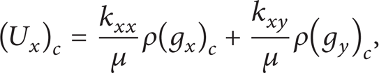
The flow simulation results by directly solving the Navier-Stokes equation are shown in Figure 2. The contours represent the magnitudes of velocity (i.e., the characteristic speed to be defined later), while the vectors represent the directions of velocity. It can be seen that the flow fields are well represented in the 9 cases. The square barriers are clearly identified by the vectors. We define characteristic speed as $V = \sqrt{U_{x}^{2} + U_{y}^{2}}$ , characteristic length as the hydraulic radius R_h = a²/(4a) = a/4, Reynolds number as Re = ρVR_h/μ, and Darcy number as Da = (R_h/L)². The characteristic parameters are listed in Table 1 (results for Samples a, b, and c are the same so that the data in Table 1 are any of them). The very low Reynolds number (order of magnitude 10⁻¹⁰∼10⁻⁸) indicates that the flows are very slow laminar flows. It can be seen that the dimensionless number ReDa^1/2 has the order of magnitude 10⁻¹¹∼10⁻⁹, which satisfies the suggested restriction of Darcy's law ReDa^1/2 ≪ 1 by Bear and Cheng [20].

Table 1:

Characteristic parameters.

Case	V (m/s)	R_h (m)	Re	Da	ReDa^1/2

Case 1	1.16 × 10⁻⁶	2.50 × 10⁻⁸	2.90 × 10⁻⁸	6.25 × 10⁻⁴	7.25 × 10⁻¹⁰
Case 2	6.62 × 10⁻⁷	5.00 × 10⁻⁸	3.31 × 10⁻⁸	2.50 × 10⁻³	1.66 × 10⁻⁹
Case 3	3.96 × 10⁻⁷	7.50 × 10⁻⁸	2.97 × 10⁻⁸	5.63 × 10⁻³	2.23 × 10⁻⁹
Case 4	2.32 × 10⁻⁷	1.00 × 10⁻⁷	2.32 × 10⁻⁸	1.00 × 10⁻²	2.32 × 10⁻⁹
Case 5	1.28 × 10⁻⁷	1.25 × 10⁻⁷	1.60 × 10⁻⁸	1.56 × 10⁻²	2.00 × 10⁻⁹
Case 6	6.24 × 10⁻⁸	1.50 × 10⁻⁷	9.36 × 10⁻⁹	2.25 × 10⁻²	1.40 × 10⁻⁹
Case 7	2.51 × 10⁻⁸	1.75 × 10⁻⁷	4.39 × 10⁻⁹	3.06 × 10⁻²	7.69 × 10⁻¹⁰
Case 8	7.12 × 10⁻⁹	2.00 × 10⁻⁷	1.42 × 10⁻⁹	4.00 × 10⁻²	2.85 × 10⁻¹⁰
Case 9	8.58 × 10⁻¹⁰	2.25 × 10⁻⁷	1.93 × 10⁻¹⁰	5.06 × 10⁻²	4.34 × 10⁻¹¹

Figure 2:

Flow fields for different porosities from Navier-Stokes simulation: columns a, b, and c represent Sample a, Sample b, and Sample c; numbers 1∼9 represent Case 1∼Case 9; the contour shows total speed while the vector shows directions of total velocity.

Porosity is defined as the ratio of void space volume to the total volume as follows:

ϕ = 1 - \frac{a^{2}}{L^{2}} .

(15)

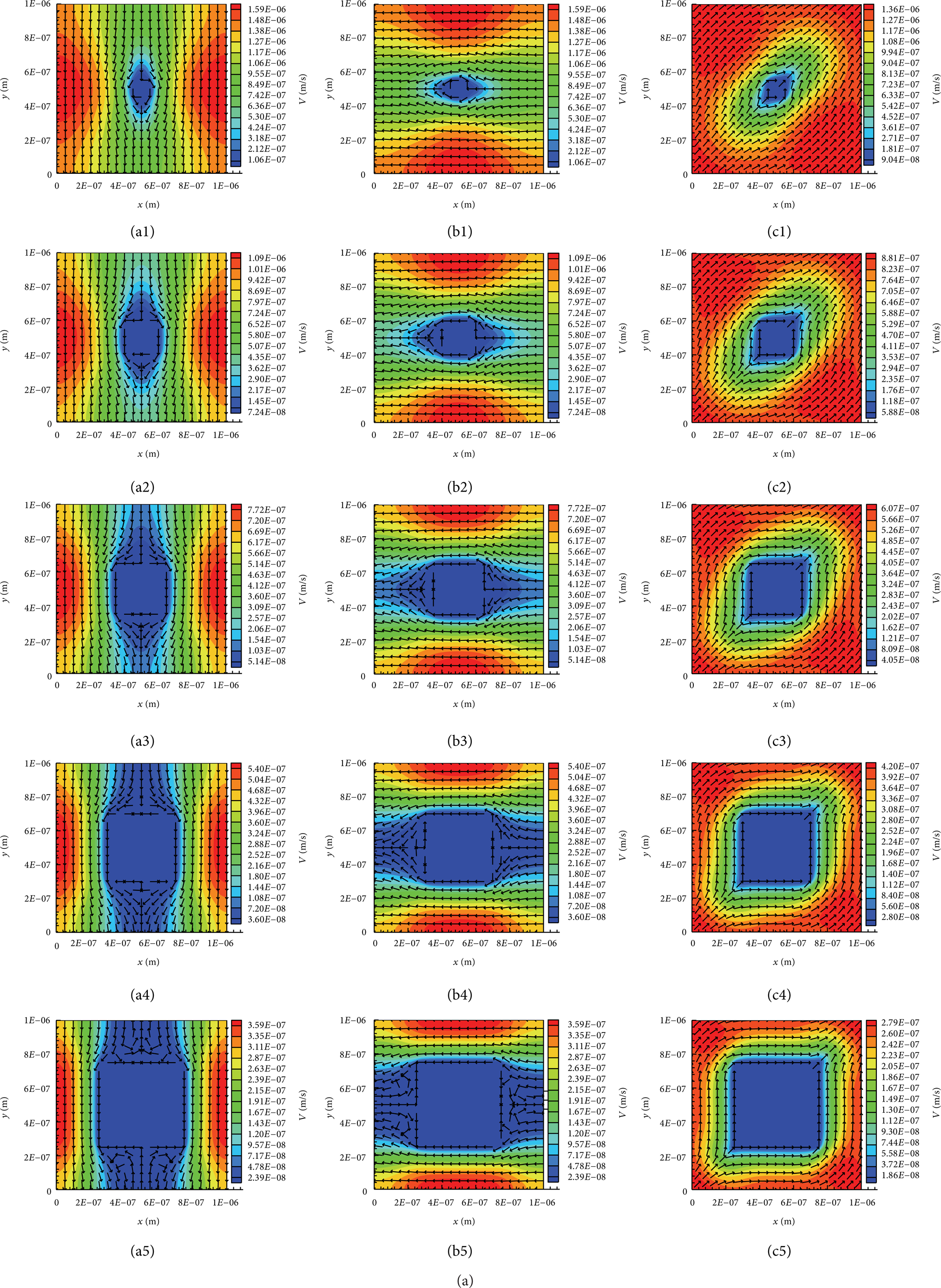
Thus, the 9 cases relate to 9 different values of porosity. Full permeability tensors obtained from flow simulation results of the 9 cases are listed in Table 2. It can be seen that the diagonal components of the permeability tensor all decrease with decreasing porosity. Their values show that the studied porous media fall within the ranges of oil rocks (10⁻¹¹ m²∼10⁻¹⁴ m²), sandstone (10⁻¹⁴ m²∼10⁻¹⁶ m²), and good limestone (10⁻¹⁶ m²∼10⁻¹⁸ m²) [20]. The diagonal components of transformed permeability tensor are shown in Figure 3 for the 9 porosities; there always exist k_ξξ = k_ηη and k_ξξ = k_xx, k_ηη = k_yy. These mean that the two diagonal components of the full permeability tensor are the same and are always equal to each other along with the rotating coordinate. This indicates that the permeable properties are all the same for any direction so that principle direction does not exist. Therefore, the full-tensor permeabilities are always diagonal tensors with equivalent components for the 9 porosities. The off-diagonal components, which are 3∼6 orders of magnitudes lower than the diagonal components (Table 2), should be considered as numerical errors. In this case, the off-diagonal components should be considered as zeros. Revealed from the mathematical meaning, physical meaning is that the porous media in the 9 cases are all isotropic. Corresponding characteristic parameters are listed in Table 3.

Table 2:

Full-tensor permeabilities at different porosities.

Case	ϕ	k_xx (m²)	k_yy (m²)	k_xy (m²)	k_yx (m²)

Case 1	0.99	1.1808 × 10⁻¹³	1.1808 × 10⁻¹³	−5.6848 × 10⁻¹⁶	−5.6363 × 10⁻¹⁶
Case 2	0.96	6.7481 × 10⁻¹⁴	6.7481 × 10⁻¹⁴	−3.1129 × 10⁻¹⁷	−2.8981 × 10⁻¹⁷
Case 3	0.91	4.0362 × 10⁻¹⁴	4.0362 × 10⁻¹⁴	−6.2013 × 10⁻¹⁹	2.6772 × 10⁻¹⁹
Case 4	0.84	2.3702 × 10⁻¹⁴	2.3702 × 10⁻¹⁴	−2.7576 × 10⁻¹⁹	3.5447 × 10⁻²⁰
Case 5	0.75	1.3026 × 10⁻¹⁴	1.3026 × 10⁻¹⁴	−8.3818 × 10⁻²⁰	1.6370 × 10⁻²⁰
Case 6	0.64	6.3596 × 10⁻¹⁵	6.3596 × 10⁻¹⁵	7.1193 × 10⁻²¹	−2.1080 × 10⁻²⁰
Case 7	0.51	2.5614 × 10⁻¹⁵	2.5614 × 10⁻¹⁵	5.8343 × 10⁻²¹	−3.6183 × 10⁻²⁰
Case 8	0.36	7.2643 × 10⁻¹⁶	7.2643 × 10⁻¹⁶	1.0640 × 10⁻²¹	−1.0052 × 10⁻²⁰
Case 9	0.19	8.7493 × 10⁻¹⁷	8.7493 × 10⁻¹⁷	6.4756 × 10⁻²³	−1.9648 × 10⁻²²

Table 3:

Characteristic permeabilities and anisotropies at different porosities.

Case	ϕ	k_max (m²)	k_min (m²)	A_k (= k_max/k_min)

Case 1	0.99	1.1808 × 10⁻¹³	1.1808 × 10⁻¹³	1.0000
Case 2	0.96	6.7481 × 10⁻¹⁴	6.7481 × 10⁻¹⁴	1.0000
Case 3	0.91	4.0362 × 10⁻¹⁴	4.0362 × 10⁻¹⁴	1.0000
Case 4	0.84	2.3702 × 10⁻¹⁴	2.3702 × 10⁻¹⁴	1.0000
Case 5	0.75	1.3026 × 10⁻¹⁴	1.3026 × 10⁻¹⁴	1.0000
Case 6	0.64	6.3596 × 10⁻¹⁵	6.3596 × 10⁻¹⁵	1.0000
Case 7	0.51	2.5614 × 10⁻¹⁵	2.5614 × 10⁻¹⁵	1.0000
Case 8	0.36	7.2643 × 10⁻¹⁶	7.2643 × 10⁻¹⁶	1.0000
Case 9	0.19	8.7493 × 10⁻¹⁷	8.7493 × 10⁻¹⁷	1.0000

Figure 3:

Diagonal components of transformed permeability tensor at different porosities.

3.2. Discussion on Reynolds Number

Besides the porosity, Reynolds number is also a key factor which may strongly affect velocity fields so that the results of permeability may be affected. Thus, it is important to check whether the Reynolds number, actually controlled by the domain size, may change the conclusions in Section 3.1. Therefore, the domain size is gradually scaled up from L = 10⁻⁶ m by keeping porosity at 0.64 (Case 6 in Tables 2 and 3). The results are shown in Table 4.

Table 4:

Full-tensor permeabilities at different Reynolds numbers.

L (m)	k_xx (m²)	k_yy (m²)	k_xy (m²)	k_yx (m²)

10⁻⁶	6.3596 × 10⁻¹⁵	6.3596 × 10⁻¹⁵	7.1193 × 10⁻²¹	−2.1080 × 10⁻²⁰
10⁻⁵	6.3596 × 10⁻¹³	6.3596 × 10⁻¹³	7.5167 × 10⁻¹⁹	−2.1064 × 10⁻¹⁸
10⁻⁴	6.3596 × 10⁻¹¹	6.3596 × 10⁻¹¹	−7.4280 × 10⁻¹⁷	−3.6338 × 10⁻¹⁶
10⁻³	6.0366 × 10⁻⁹	6.0366 × 10⁻⁹	−1.9077 × 10⁻⁹	−1.9077 × 10⁻⁹
≥10⁻²	Divergence	Divergence	Divergence	Divergence

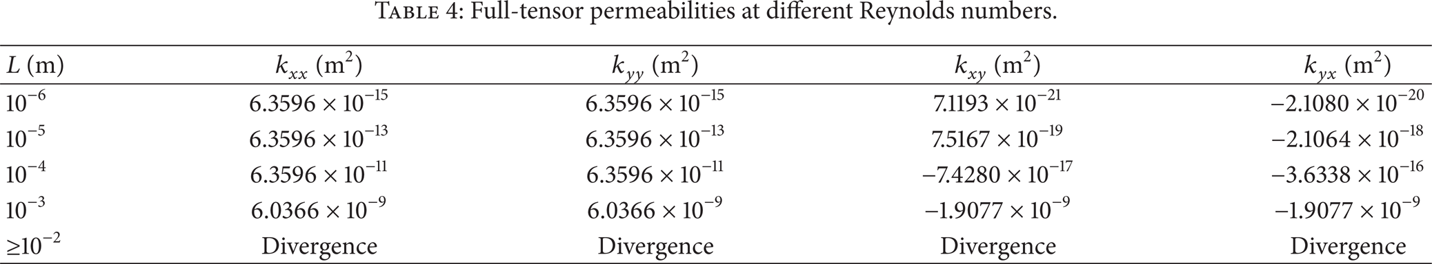
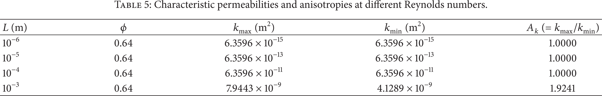
From 10⁻⁶ m to 10⁻⁴ m, the diagonal components of the full-tensor permeability just increase two orders of magnitudes once the domain size increases one order of magnitude. The off-diagonal components should still be considered as numerical errors and set to be zeros as stated previously. These three cases are quite similar, and their difference is only the magnitude. It can be verified by the flow fields in Figures 4(a1), 4(b1), 4(c1)∼Figures 4(a3), 4(b3), 4(c3), Figures 5(a)∼5(c), and Table 5 that the domain size scaling up from 10⁻⁶ m to 10⁻⁴ m just leads the velocity to increase proportionally. They are all isotropic. However, the situation is different when the domain size increases up to 10⁻³ m (see line 5 in Table 4). The off-diagonal components are no longer several orders of magnitudes smaller than the diagonal components so that the full-tensor permeability is no longer diagonal. Figures 4(a4)∼4(c4) show that the fluid tends to depart the solid walls and the vortex expands. Figure 5(d) shows that the components of the transformed permeability tensor are no longer constant. Maximum and minimum values of the diagonal components (k_max, k_min) can always be obtained at the same time once the off-diagonal components become zeros. Their values (Table 5) show that the porous media at the domain length of 10⁻³ m enter the range of clean stand (10⁻⁹ m²∼10⁻¹² m²) which is a better aquifer than the previous ones [20]. Correspondingly, four angles (α_I,α_II, α_III, and α_IV) can be obtained, which are shown in Table 6. Surprisingly from Table 5, the porous media start to show anisotropic property (A_k = 1.9241) when the domain length reaches 10⁻³ m. It can be summarized from Table 6 that α_p is always equal to angle α_II or α_IV when k_max equals k_ξξ. These two angles are on the same line across the second and the fourth quadrants in the original xOy coordinate (see Figure 1(c)). This line is the direction where permeability achieves maximum value, that is, the easiest directionwhere fluid can pass through, so that this is the principle direction. Accordingly, the direction fluid receives the most resistance (i.e., the direction for k_min) is the line represented by angles α_I and α_III, so that this line is the direction orthogonal to the principle direction.

Table 5:

Characteristic permeabilities and anisotropies at different Reynolds numbers.

L (m)	ϕ	k_max (m²)	k_min (m²)	A_k (= k_max/k_min)

10⁻⁶	0.64	6.3596 × 10⁻¹⁵	6.3596 × 10⁻¹⁵	1.0000
10⁻⁵	0.64	6.3596 × 10⁻¹³	6.3596 × 10⁻¹³	1.0000
10⁻⁴	0.64	6.3596 × 10⁻¹¹	6.3596 × 10⁻¹¹	1.0000
10⁻³	0.64	7.9443 × 10⁻⁹	4.1289 × 10⁻⁹	1.9241

Table 6:

Angles at zero off-diagonal components of transformed permeability for L = 10⁻³ m.

L (m)	α_I	α_II	α_III	α_IV	α_p

10⁻³	45°	135°	225°	315°	135°, 315°
Summary	k_max = k_ηη k_min = k_ξξ	k_max = k_ξξ k_min = k_ηη	k_max = k_ηη k_min = k_ξξ	k_max = k_ξξ k_min = k_ηη	α_p = α_II or α_IV

Figure 4:

Flow fields for different Reynolds numbers from Navier-Stokes simulation: columns a, b, and c represent Sample a, Sample b, and Sample c; numbers 1∼4 represent domain size L = 10⁻⁶ m, 10⁻⁵ m, 10⁻⁴ m, and 10⁻³ m, respectively; the contours show total speed while the vectors show directions of total velocity.

Figure 5:

Components of transformed permeability tensor at different Reynolds numbers: (a) L = 10⁻⁶ m, (b) L = 10⁻⁵ m, (c) L = 10⁻⁴ m, and (d) L = 10⁻³ m.

When the length of domain is greater than or equal to 10⁻² m, the flow simulation is divergent. This is probably because the mesh size 80 × 80 is not dense enough for larger domain. Larger domains with finer grid, which are very time consuming, will be studied in the future.

To discuss the previous phenomenon that different Reynolds numbers may generate essentially different permeability tensors, or in other words predict different types of porous media for the same configuration, four characteristic parameters are shown in Table 7. R_u and R_v are defined as the ratios of the mean convection effect to the mean diffusion effect in the momentum equation (2):

\begin{matrix} R_{u} = \frac{\overset{—}{u (\partial u / \partial x) + v (\partial u / \partial y)}}{\overset{—}{(μ / ρ) (\partial^{2} u / \partial x^{2} + \partial^{2} u / \partial y^{2})}}, \\ R_{v} = \frac{\overset{—}{u (\partial v / \partial x) + v (\partial v / \partial y)}}{\overset{—}{(μ / ρ) (\partial^{2} v / \partial x^{2} + \partial^{2} v / \partial y^{2})}}, \end{matrix}

(16)

where the superscript “—” represents the average value over the whole domain. It is clear in Table 7 that the fluid flows are actually diffusion dominated for the domain lengths smaller than 10⁻³ m since R_u and R_v are all much smaller than 1. However, R_u and R_v are greater than 1 at the domain length of 10⁻³ m. This means that the flow is dominated by the convection effect of fluid. It is well known from their intentions that the diffusion effect tends to transport variables to all directions uniformly while the convection effect tends to transport variables along specific directions. Therefore, the existence of convection dominant flow may be the main reason for the anisotropy. It is worth to point out that Table 7 also verifies the conclusion made by Bear and Cheng[20] that Darcy's law is usually valid as long as Reynolds number is lower than 1 (occurred at the domain lengths 10⁻⁶ m∼10⁻⁴ m where Re = 9.36 × 10⁻⁹∼9.36 × 10⁻³) but sometimes as high as 10 (occurred at the domain length 10⁻³ m where Re = 8.88 and the suggested restriction ReDa^1/2 ≪ 1 is violated).

Table 7:

Characteristic parameters at different Reynolds numbers.

L (m)	Re	ReDa^1/2	R _u	R _v

10⁻⁶	9.36 × 10⁻⁹	1.40 × 10⁻⁹	2.79 × 10⁻⁹	2.79 × 10⁻⁹
10⁻⁵	9.36 × 10⁻⁶	1.40 × 10⁻⁶	2.79 × 10⁻⁶	2.79 × 10⁻⁶
10⁻⁴	9.36 × 10⁻³	1.40 × 10⁻³	2.79 × 10⁻³	2.79 × 10⁻³
10⁻³	8.88	1.33	1.35	1.35

4. Conclusion

A numerical method is proposed to compute the permeability in the form of full tensor. The flow simulation results show that flow fields can be well represented by solving the Navier-Stokes equation directly. Original and transformed permeability tensors are obtained so that maximum and minimum components of permeability with principle directions and anisotropies are detected successfully. With this information, the directions of largest and smallest resistances for fluid flow in porous media can be inferred easily.

Through the analyses on the porosity effect and the Reynolds number effect, it is found that porous media with the same porosity and the same configuration can manifest different levels of anisotropy at different Reynolds numbers. At the Reynolds numbers that diffusion dominates flow, isotropy is a good description. At the Reynolds number that convection dominates flow, anisotropy occurs. Thus, it is important to pay attention to Reynolds numbers for porous media applications. This is especially important for applications with large Darcy velocities, such as flow and transport in packed columns and in fractured geological media.

5. Future Issues to Be Addressed

The previous discussions show that the proposed method in the present study is an easy way to determine full-tensor permeability numerically and related characteristics. However, many issues still need to be addressed in future works. Only two of them are briefly listed below as an example.

Method for solving the Navier-Stokes equation in porous media should be improved to accelerate the computation. Current speed is not acceptable for engineering applications. Multigrid method needs to be developed for the flow around solids so that the iteration of pressure can be largely accelerated. High-resolution time integration scheme is expected to largely reduce the number of time steps needed. Since only steady-state results are needed for obtaining the full-tensor permeability, a method directly solving the steady-state Navier-Stokes equation is also expected so that a large amount of time integrations can be avoided.

Shape, number, position, and so forth of inner barriers should be intensively studied to know the application and limitation of this method and to improve precision. Denser meshes are also expected to study what will happen for larger Reynolds numbers.

Footnotes

Acknowledgments

The work presented in this paper has been supported in part by the project entitled “Simulation of Subsurface Geochemical Transport and Carbon Sequestration,” funded by the GRP-AEA Program at KAUST. The work has also been supported in part by National Science Foundation of China (no. 51206186, no. 51174206) and Science Foundation of China, University of Petroleum, Beijing (no. 2462012KYJJ0403, no. 2462012KYJJ0404).

References

Dinwiddie

C. L.

Molz

F. J.

III , and Castle

J. W.

, “A new small drill hole minipermeameter probe for in situ permeability measurement: fluid mechanics and geometrical factors,” Water Resources Research, vol. 39, no. 7, 2003.

Wolfson

B. J.

and Wentworth

S. M.

, “Complex permeability and permeability measurement using a rectangular waveguide,” Microwave and Optical Technology Letters, vol. 27, no. 3, pp. 180–182, 2000.

Ivanov

A. N.

Kozlova

S. N.

, and Pechenov

A. V.

, “Permeability measurement,” Measurement Techniques, vol. 43, no. 12, pp. 1086–1088, 2000.

Jensen

J. L.

and Heriot-Watt

, “A model for small-scale permeability measurement with applications to reservoir characterization,” in Proceedings of the SPE/DOE 7th Symposium on Enhanced Oil Recovery, pp. 891–900, April 1990.

Wang

T. J.

C. H.

, and Lee

L. J.

, “In-plane permeability measurement and analysis in liquid composite molding,” Polymer Composites, vol. 15, no. 4, pp. 278–288, 1994.

Ferland

Guittard

, and Trochu

, “Concurrent methods for permeability measurement in resin transfer molding,” Polymer Composites, vol. 17, no. 1, pp. 149–158, 1996.

Gauvin

Trochu

Lemenn

, and Diallo

, “Permeability measurement and flow simulation through fiber reinforcement,” Polymer Composites, vol. 17, no. 1, pp. 34–42, 1996.

Luo

Verpoest

Hoes

Vanheule

Sol

, and Cardon

, “Permeability measurement of textile reinforcements with several test fluids,” Composites A, vol. 32, no. 10, pp. 1497–1504, 2001.

Fwa

T. F.

Tan

S. A.

Chuai

C. T. Y.

, and Guwe

, “Expedient permeability measurement for porous pavement surface,” The International Journal of Pavement Engineering, vol. 2, pp. 259–270, 2001.

10.

Arbter

Beraud

J. M.

Binetruy

, “Experimental determination of the permeability of textiles: a benchmark exercise,” Composites A, vol. 42, no. 9, pp. 1157–1168, 2011.

11.

Weitzenböck

J. R.

Shenoi

R. A.

, and Wilson

P. A.

, “Measurement of principal permeability with the channel flow experiment,” Polymer Composites, vol. 20, no. 2, pp. 321–335, 1999.

12.

Weitzenböck

J. R.

Shenoi

R. A.

, and Wilson

P. A.

, “Radial flow permeability measurement. Part A: theory,” Composites A, vol. 30, no. 6, pp. 781–796, 1999.

13.

Weitzenböck

J. R.

Shenoi

R. A.

, and Wilson

P. A.

, “Radial flow permeability measurement. Part B: application,” Composites A, vol. 30, no. 6, pp. 797–813, 1999.

14.

Keehm

Mukerji

, and Nur

, “Computational rock physics at the pore scale: transport properties and diagenesis in realistic pore geometries,” Leading Edge, vol. 20, no. 2, pp. 180–183, 2001.

15.

Kameda

Dvorkin

Keehm

Nur

, and Bosl

, “Permeability-porosity transforms from small sandstone fragments,” Geophysics, vol. 71, no. 1, pp. N11–N19, 2006.

16.

Saenger

E. H.

Enzmann

Keehm

, and Steeb

, “Digital rock physics: effect of fluid viscosity on effective elastic properties,” Journal of Applied Geophysics, vol. 74, no. 4, pp. 236–241, 2011.

17.

Quintal

Frehner

Madonna

Tisato

Kuteynikova

, and Saenger

E. H.

, “Integrated numerical and laboratory rock physics applied to seismic characterization of reservoir rocks,” Leading Edge, vol. 30, no. 12, pp. 1360–1367, 2011.

18.

Keehm

Mukerji

, and Nur

, “Computational rock physics at the pore scale: transport properties and diagenesis in realistic pore geometries,” Leading Edge, vol. 20, no. 2, pp. 180–183, 2001.

19.

Bishop

R. L.

and Goldberg

S. I.

, Tensor Analysis on Manifolds, Dover Publications, 1968.

20.

Bear

and Cheng

A. H. D.

, Modeling Groundwater Flow and Contaminant Transport, vol. 23 of Theory and Applications of Transport in Porous Media, Springer Science+Business Media B.V., 2010.

On Full-Tensor Permeabilities of Porous Media from Numerical Solutions of the Navier-Stokes Equation

Abstract

1. Introduction

2. Principles and Methods

2.1. General Principles

2.2. Numerical Methods

3. Results and Discussion

3.1. Discussion on Porosity

3.2. Discussion on Reynolds Number

4. Conclusion

5. Future Issues to Be Addressed

Footnotes

Acknowledgments

References