
Abstract
Continuous k-nearest neighbor (CkNN) search is a variation of kNN search that the system persistently reports k nearest moving objects to a user. For example, system continuously returns 3 nearest moving sensors to the user. Many query processing approaches for CkNN search have been proposed in traditional environments. However, the existing client-server approaches for CkNN search are sensitive to the number of moving objects. When the moving objects quickly move, the processing load on the server will be heavy due to the overwhelming data. In this thesis, we propose a distributed CkNN search algorithm (DCkNN) on wireless sensor networks (WSNs) based on the Voronoi diagram. There are four features about DCkNN: (1) each moving object constructs a local Voronoi cell and keeps the local information; (2) in order to keep the reliability of system, the query message will be propagated to related objects; (3) using the idea of safe time, the number of updates is reduced; (4) an equation to estimate a more accurate safe time is provided. Last, we present our findings through intensive experiments and the results validate our proposed approach, DCkNN.
1. Introduction
The mobile sensors have been widely used in recent years. For example, the smartphone, Samsung Galaxy S4, includes a barometer, thermometer, and hygrometer (to measure humidity)—the first major smartphone to do so. By using these sensors, people can easily use their mobile devices to obtain environmental information. On the other hand, the popularization of global positioning system (GPS) and the miniaturization of mobile devices, equipped with a wireless network module, make location-based services (LBSs) no longer expensive. Thus, with the combination of the mobile sensors and the GPS, more and more interesting applications and issues gradually emerged.
In general, one can regard each mobile device (sensor) as a moving object in wireless mobile sensor networks. Each user (object) can use the GPS and sensors to provide the environmental information, such as location, temperature, and humidity, to the information systems which are built by the manufacturers. These systems can sink user's information and send the user's location through the mobile networks. Mobile users can immediately access the information related to the location and geographic information. Many manufacturers even provide different telecommunication services to the users, The multiple types of information services make life more convenient. For example, if a user issues a query and wants to know the temperature at a specific location, the neighboring mobile objects of this location will return the measured temperature information to the user. Another example is the temperature monitoring system where a mobile sink may move around to collect the temperature around it. In these cases, the query may move.
As the above examples, the mobile query often selects k nearest neighbors (kNN) [1] around itself to obtain the average of the measured temperatures. Moreover, the mobile query may monitor the environmental information for a period of time. Each moving object thus needs to continuously reply to the mobile query with measured environmental information and location. Such an application actually is the continuous k nearest neighbors (CkNN) query [2, 3], which is used to derive the k nearest neighbor sensors and then get the average of the received information continuously. In this paper, we consider the mobile environment where the data objects and queries can move.
Spatial queries, such as k nearest neighbors query and continuous k nearest neighbors query, have attracted many researchers' interest and also have been discussed on many different applications. Most of the existing methods about the kNN or CkNN search in the considered mobile environment still use the client-server architecture and rely on a central server for processing queries. Each moving object needs to continuously obtain the location information of itself by GPS and send the information back to the server for updating the database. Thus, if we use the existing methods under a specific scenario that the position status of objects changes frequently, the server must receive a huge amount of information stream for updating each object's location in a short time, thus causing the server system to be overloaded. Besides, the large amount of messages for updates occupies quite a lot of bandwidth. We hence propose an effective and noncentralized approach for supporting CkNN query in a mobile environment.
In this work, we consider the continuous k nearest neighbors query in WSNs or some other distributed and mobile environments like WSNs, which consist of a number of mobile devices (sensors) and propose a new distributed approach, DCkNN, for processing CkNN query efficiently. From the object's point of view, the distributed architecture using local computation can effectively reduce the updating cost since the update messages in the client-server architecture may need more hops to arrive to the server. Even worse, the long delay of the update messages can make the answer of the CkNN inaccurate. On the other hand, the distributed architecture can avoid the long response time caused by the overload of the server. In our considered environments, each mobile device, also called moving sensor or moving object, can obtain its location information by the GPS equipment. Besides, each moving object is equipped with enough storage and a cpu for storing the local information and processing simple 2D functions, respectively.
In our proposed approach, each moving object will send messages to its one-hop neighbors when necessary to avoid the wrong information for processing spatial queries. When finding the kNN, our method uses the incremental strategy on the number of hops based on the Voronoi diagram (VD) [4]. In order to estimate the movement of a moving object accurately, we consider the speed of each moving object and adapt the concept of safe region [5] to our proposed approach, distributed continuous k nearest neighbors (DCkNN).
In this paper, we address the problem of efficiently processing continuous k nearest neighbors over moving objects with updates and make the following contributions.
We identify the continuous k nearest neighbors search problem on mobile ad hoc networks and categorize some detailed existing works about this issue. We provide a novel approach, using local Voronoi diagram, for efficiently and precisely collecting the location of each object in a distributed way. With the combination of local Voronoi diagram, we propose a model for accurately estimating the safe-time (safe-region) of continuous k nearest neighbors query, which can lead to a short response time, fewer number of messages, less update cost, and high accuracy. We perform a simulated experimental evaluation and the results show the superiority of our solution over the adaptation of state-of-the-art solutions [5] given to the similar issues.
The rest of this paper is organized as follows. In Section 2, we review the related work. The performance metrics and considered issues are introduced in Section 3. Section 4 presents the proposed solution using localized Voronoi diagram and how to derive the accurate safe time. Section 5 gives some analysis and comparisons between the proposed DCkNN method and different existing methods. The discussion on the experimental simulation is in Section 6. Finally, we give the conclusion remarks in Section 7.
2. Related Work
The existing works for CkNN search can be categorized into the following categories according to the ways for accessing or managing data: (1) pull-based approach, (2) push-based approach, and (3) distributed and mobile approach. The pull-based approach uses the traditional client-server architecture [6–8]. A given central server is responsible for processing the spatial queries from the user devices and all the data are stored in the server. Whenever a client wants some information, the client will send a query to the server. In many applications, the amount of spatial data needed to be processed could be very large and hence the spatial data is usually saved in the external storages, such as disks. Thus, the existing approaches for CkNN search using the pull-based approach focus on optimizing the number of I/O's. Of course, the computation time (CPU time) is still an important performance metric when the size of spatial data needed to be processed is not large. As a result, the above two measurements, the number of I/O's and CPU time, are usually used to validate the effectiveness of the proposed algorithms for processing kNN and CkNN queries using pull-based approach. However, the bandwidth of communication between the clients and servers is asymmetric. In other words, the uplink bandwidth is limited and much smaller than the bandwidth of downlink. This phenomenon in wireless communication will cause the bottleneck [9] when the number of queries increases if the pull-based approach is applied for accessing data.
In order to overcome the bottleneck problem caused by the pull-based approach in wireless environment, the push-based approach is proposed and also referred to as data broadcasting approach. Data broadcasting has attracted a lot of research attention in the past decades and many approaches or protocols for different types of spatial queries have been proposed [10–13]. In the data broadcasting environment, the data are broadcast in the air by the server and the clients execute the query process by listening to the broadcast channel. The load for processing data on the server is dramatically decreased and relieves the bottleneck problem. Instead, the computation load on the clients is increased. From the user's point of view, the fewer battery power each device consumes, the better experience each user has. Thus the existing works [10, 11, 13–15], in general, discuss the performance of data broadcasting protocol in terms of latency and tuning time. Latency is the time a client experiences from issuing query to receiving the complete answer. The tuning time is the amount of time actually spent on listening to the broadcast. The latency indicates the quality of service (QoS) provided by the system and the tuning time can represent the power consumption of mobile clients.
Many works [16–18] have discussed the kNN and CkNN queries on the distributed and mobile environments like mobile ad hoc NETworks (MANETs) and wireless sensors networks (WSN). MANETs and WSNs are self-configuring infrastructure-less networks consisting of mobile devices and sensors connected by wireless communication. Each device in such networks is free to move independently in any direction and will thus change its links to other devices frequently. Each device can forward the traffic unrelated to its own use and act as a router. In contrast to the client-server and data broadcasting environments, there is no central server that handles the spatial queries or broadcasts spatial data in MANETs or WSNs. Accordingly, the information system based on the above infrastructure-less networks has to process the queries in a distributed way. Each mobile node (or device) in such a system cooperates and exchanges spatial data with each other and then derives the answer for the spatial queries.
In spatiotemporal data applications, the datasets consist of data objects and the data as well as queries might move over time. In order to process a great volume of spatial data and queries efficiently, some decomposition methods, such as grid and Voronoi diagram, have been used in the existing works [7, 19, 20]. Xiong et al. [20] focused on multiple kNN queries and proposed an incremental search technique based on hashing objects into a regular grid and keeping CPU time in mind. The main objective of this work on disk-resident data is to minimize disk I/O operations. The CPU time is considered only as a secondary objective. Zhao et al. [21] proposed a Voronoi-based approach for CKNN query. Although this work provided a navigation service to mobile devices, the query processing is still operated on a central server.
Mouratidis et al. [22] proposed a threshold-based algorithm to help the server processing continuous nearest neighbor queries from geographically distributed clients. Within a given threshold, the k nearest neighbors of the query point will not change. However, this work still needs a central server for monitoring the kNN objects, maintaining the huge spatial data, and broadcasting each object's information. Chatzimilioudis et al. [16] proposed a proximity algorithm to answer all k-nearest neighbor queries continuously. In such an environment, many stations, called query processors, are placed to monitor all the objects in the radio region. Then, different query processors can exchange the monitored spatial information to calculate the k nearest neighbor answer to the user (query point).
In contrast to most of the above approaches, Kim et al. [5] proposed a decentralized method to support continuous k nearest neighbor query. Each query object predicts a safe time as a threshold for reducing the cost of information update. This method assumes that there is a maximum speed, MaxSpeed, of each object in the environment and use, DIKNN algorithm [23] to find the initial k nearest neighbors. By monitoring the kth and
3. Preliminaries
In this section, we present some concepts and techniques that are generally used when solving the spatial data queries on moving objects. The metrics generally used to evaluate the query process will also be introduced.
3.1. Spatial Query
The k nearest neighbor search (kNN search) is one of the important types of spatial queries. Suppose that the distance between two points v and u is

A 2NN search with query point q, where 2NN
Definition 1 (kNN search problem).
Given a query point q and an integer k, the k NN search problem is to find a subset
The continuous k nearest neighbors search (CkNN Search) [3] is a variation of kNN query. CkNN search is extended from kNN search and the system will continuously return the kNN answer in a time interval. In a mobile environment, the mobile devices are regarded as moving objects. Thus, the result of a CkNN search may change over time due to the movement of the queries and data objects. We can model the moving pattern of the query as a path consisting of consecutive line segments and then consider the line segments for CkNN search. Let D be a dataset of data objects and

An example of CkNN,
Definition 2 (CkNN search problem).
Given a line segment
3.2. Voronoi Diagram
Using Voronoi diagram (VD) for CkNN search is proposed in the pull-based approach [7]. Consider a set P of n distinct data points, called sites, in the plane. The Voronoi diagram of P, denoted by
A continuous nearest neighbor search example using Voronoi diagram.
Using the Voronoi diagram, one can easily find the NN for a query point. To find the kNN for an arbitrary

The construction of an approximate order-3 Voronoi cell, where q is the query point.
3.3. Safe-Time
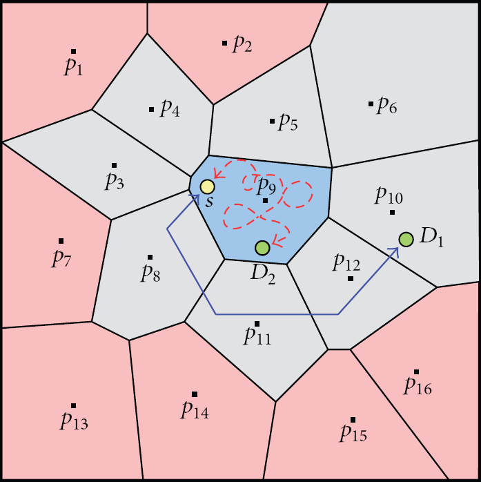
In the wireless sensor network, the idea of safe-time is proposed by Kim et al [5]. This method first assumes that there is a maximum speed, MaxSpeed, of each object in the environment and then uses DIkNN algorithm [23] to find the initial k nearest neighbors. As Figure 5 shows, the user located at S issues a query with q as the center point of this query. The system will first inquiry object

The kNN search on WSNs: (a) Q-node is the first object receiving the query and D-node is the sink node which is responsible for collecting data and (b) presents the multihops routing path for the kNN process.

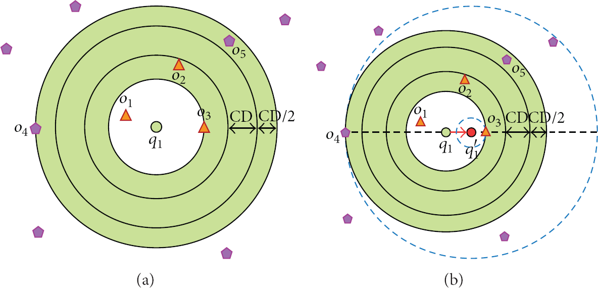
Update process using safe-time for 3NN search on WSNs: (a) shows the CD between the third and fourth closest data points; (b) presents the maximum influenced distance for update using broadcast; (c) indicates the area for broadcasting to update.
3.4. Performance Metrics
In order to evaluate the proposed DCkNN approach, we consider the following performance metrics, including update cost, number of messages, accuracy, and response time.
3.4.1. Update Cost
The update cost is to measure the number of updates during the query process. We sometimes use the frequency to denote it. Since the sensors (objects) and even the query will move, the status of the sensors should be maintained in order to have the accurate results. However, the cost for one update is high in the distributed environment. Hence, one of the objectives of the designed algorithm, DCkNN, is to minimize the update cost for the CkNN query.
3.4.2. Number of Messages
Except for the number of updates, there are some other kinds of messages for the query process in the distributed and mobile environment, including the messages for query and information passing. The total number of messages used during the query process can be used to indicate the throughput over the networks and the energy consumption. So the proposed DCkNN is towards minimizing the total number of messages for the query.
3.4.3. Accuracy
By using the pull-based approach, the time interval for routing update messages to the server depends on the distance between the data object and the server. It thus can not ensure that the location information of each object saved in the server is the latest. Hence, the results may be timely incorrect when deriving the answers for a query due to the mobility. This situation becomes worse in the distributed and mobile environments. In our design, the proposed approach can avoid redundant updates and keep the accuracy of the results.
3.4.4. Response Time
The complicated query process, the delay time for message communication, and the number of users will affect the response time of the system to process the query. Long response time is unbearable and may return obsoletely invalid query results. Even worse, the long response time may cause important information missing or financial loss. Thus the system response time is also one of the important issues that must be considered when designing the method for continuous queries.
4. Distributed Continuous k Nearest Neighbors Search
In the mobile and distributed environments, like WSNs or MANETS, the pull-based approach may not be a good match for CkNN search due to the problems discussed in Section 2. We thus propose a distributed algorithm, DCkNN, for CkNN search in the mobile and distributed environments. The distributed approach using a better safe-time can reduce the update cost, relieve the load for server, shorten the response time, and make the result more accurate. There are three phases in DCkNN: initialization phase, query processing phase, and information update phase. In the initialization phase, each moving object exchanges the location information and builds a local Voronoi cell (LVC) as well as calculates the safe time for the LVC. The query processing phase collects sufficient location and environmental information of neighboring neighbors for exploring the result of the given CkNN query. The last information update phase is to maintain the latest information for the moving objects and the result of the continuous k nearest neighbor query. The following will explain each phase in details.
4.1. Phase 1: Initialization
During system initialization, each mobile sensor (moving object) exchanges location information with its neighbors, derives the local Voronoi cell (LVC), calculates the safe time of LVC, and then stores the LVC and safe time in the memory.
When a user issues an NN query Q and broadcasts the query message
4.2. Phase 2: CkNN Query Processing
The pseudocode, Query_DCkNN_Search(), in Algorithm 1 shows the whole query process on the query point. The operations from Line 6 to the end of Query_DCkNN_Search() do the query processing of CkNN
(1) broadcast a query (2) get the Voronoi cells or object's information; (3) (4) show LVC; (5) find (6) (7) (8) broadcast the query (9) run normal kNNSearch to find kNN set; (10) show LVC according to kNNset and (11) find (12) (13) wait;
When the received information is enough to derive the results of kNN, the query point Q will use the approximate method we modified from [25] to calculate the approximate order-k LVC in which the query point Q locates. By using the modified method, the query point Q has to partition the plane into λ equal sectors and selects an additional nearest neighboring object in each sector, excluded from kNN objects. Thus, the query point Q needs to collect at least
Figure 7 gives an example for the case of
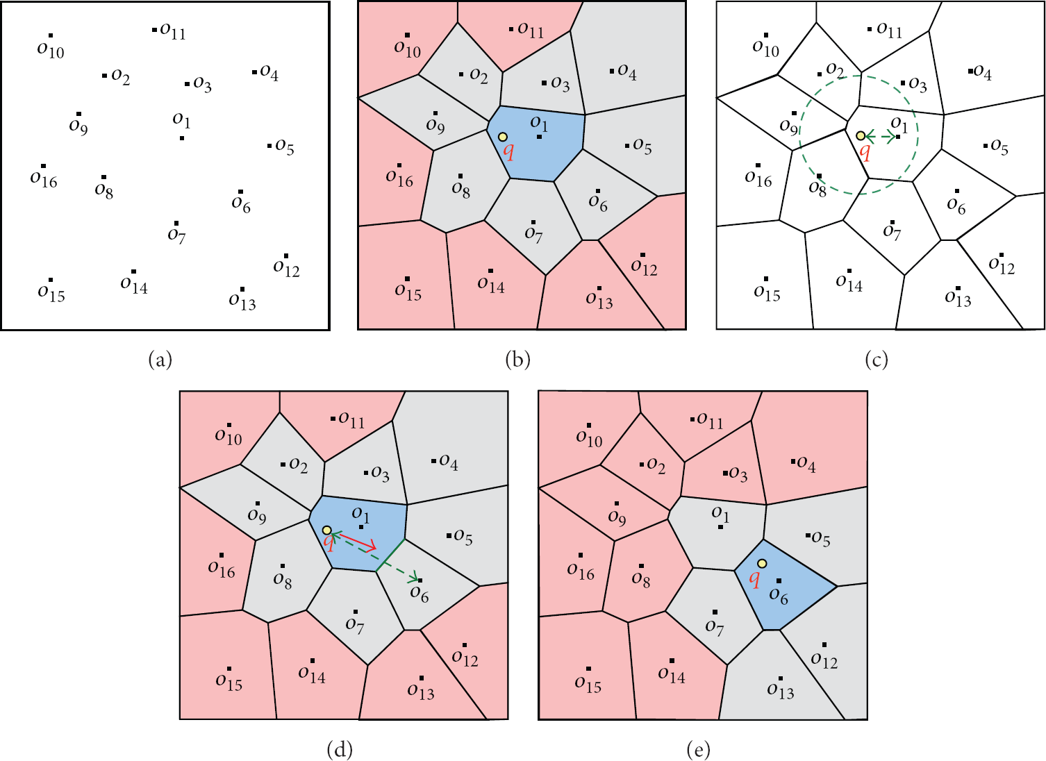
An example of DCNN where (a) each sensor exchanges information in the initial step; (b) each sensor builds its LVC; (c) a query at object q is issued and sensor
Figure 8 demonstrates an example of DCkNN for

An example of DCkNN for
4.3. Phase 3: Information Updates
In the distributed and mobile environments, it is challenging for a mobile node to maintain the location information of the other mobile nodes effectively. If a mobile node sends the update messages frequently, it will consume much network resource and power. Furthermore, the result of the moving query should be effectively maintained. For different roles, nodes, and query, we propose effective ways, respectively, in our DCkNN query process to update the location information and maintain the query result.
4.3.1. The Safe Time of Each Object
In the proposed approach, DCkNN, each object cooperates with each other and exchanges information to update the location information of each object. In order to monitor and obtain the continuous answer of a continuous k nearest neighbors query, we use a safe distance between each object and query. Then we can derive the safe time of each object for location updates by estimating the maximum speed of that object. Suppose that the sensing area is partitioned into a grid for location management. There are three possible methods for deriving the safe distance. The first one is the grid-based safe distance. Each object directly uses the minimum distance between itself and the boundary of the grid cell where the object locates. Simply using the grid-based safe distance may cause some problems about the imprecise updates. The second method, VD-based safe distance, uses VD to obtain the safe distance. In order to predict the safe distance more precisely, we can consider the previous two distances simultaneously and then select the smaller one. So the last method, proper safe distance, will return a better safe distance by comparisons. Having the safe distance, the safe time then can be derived by estimating the maximum speed of the considered object.
In Figure 9, the sensing area is divided into a grid and the Voronoi diagram formed by the sensors is also shown. For sensor
An illustration for different safe distances: (a) sensor
4.3.2. The Safe Time of Each Query
For the moving query, it is important to know when the result will change. To derive the safe time, during which the result will not change, we refer to the characteristics of Voronoi diagram. In the traditional environment with static objects, the system only uses the minimum distance from the query to the boundary of the Voronoi cell where the query locates as the safe distance. The the safe time can be obtained by the estimated maximum speed of that query. During the safe time, no update is necessary, thus saving the update cost.
Unfortunately, in the moving object environment, the above method cannot obtain the right safe time. As shown in Figure 10, the left part shows the static case, where L is the Voronoi cell boundary between objects A and B, and the safe distance of the query can be calculated as the figure shows. However, for the moving objects, the original safe distance between the L and query cannot be directly used to calculate the safe time because the object movement will cause the distance form query to L to be nonlinearly increasing or decreasing. As the right part of Figure 10 shows, after the movement of object A and object B, L becomes

An example showing the impact on the safe distance caused by object movement.
In order to derive the precise safe distance, we consider the movements of objects and query simultaneously and use Figure 11 to illustrate. Initially,

The precise safe-time for moving objects A and B and the moving query, where (a) shows the beginning state, (b) presents the moment when the moving query meets the boundary, and (c) gives the diagram for the change on the safe distance with time t.
In the following, we present the way to calculate the safe time when
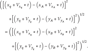
Then,

Equation (2) is a quadratic equation. Since a general quadratic equation can be written in the following form:

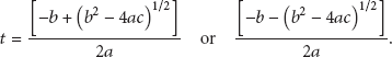
Finally, we select the minimum value of
Additionally, assuming that d is the distance between the object and the query and t is the time,
5. Comparisons with Previous Approaches
In this section, we compare the proposed DCkNN approach, the Safe-time with stationary query approach [5], and the naïve way used pull-based approach, in terms of safe time, space, and accuracy.
5.1. Safe Time
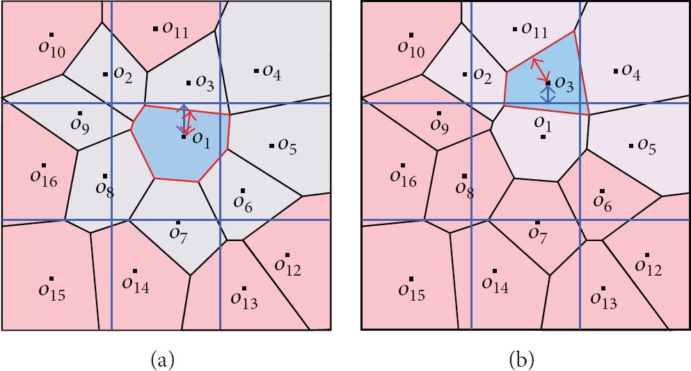
The original safe-time with stationary query [5] (safe-time(S)) does not support moving queries. An example of C3NN is shown in Figure 12, where
The phenomenon when using the original safe-time methods to (a) stationary query and (b) moving query.
We adapt the safe-time(S) method for moving query. The adapted approach will result in a higher update cost. Figure 12(b) presents a case that the query moves toward object
In addition, according to the Figure 12(b), we can know that the original Safe-time method, safe-time(S), is not appropriate for moving queries since the calculation of Safe-time(S) method does not consider the speed of query. safe-time(S) directly uses twofold of the maximum speed of the kth and
We modify the Safe-time to fully support the moving query. In order to support and maintain the accuracy of moving query, the maximum speed (Maxspeed) used in the safe time calculation is required to be modified and replaced by the maximum relative speed between the query and the objects. Because of using the relative speed, the adapted safe-time method, safe-time(M), needs twofold maximum relative speed (
5.2. Space
In DCkNN, each object and query only need to maintain the information of LVC. The information to be stored includes the location of neighboring objects and the object information of order-k's local Voronoi diagram. The total amount of stored information is not significant on each object. Thus, the use of storage space does not need to be very substantial.
5.3. Accuracy
The safe-time (S) [5] considers the stationary query. When applying it to the moving query, some adaption should be made. According to our experimental results, when the value of k increases with a moving query, the accuracy of the result will be reduced. In our simulation, we modify the original Safe-time(S) as Safe time(M) for moving query and consider the relative distance in detail caused by the moving query and objects. Although the correctness of the answer can be increased, the update frequency increases, thus increasing the number of delivered messages.
DCkNN uses Voronoi and grid cell boundary to calculate the safe time and updates the information of related objects before the end of the safe time. In fact, the boundary of the Voronoi cell represents the boundary of moving kNN query. After the safe time period, the query will collect the information of related neighboring objects. Having such real-time information, the query can have the result more accurate in time. Similar to safe-time(M), DCkNN uses the kth and
6. Simulation Experiments
In the simulation, we compare the following methods: Naïve, DCkNN, safe-time (S), and safe-time (M). The Naïve method is centralized and used as a benchmark for the comparison. All the mobile sensors will send the location information to the central server to update the information. The other methods, DCkNN, Safe-time(S), and Safe-time(M), are distributed and used in the considered mobile wireless sensor network, where each object knows its position, has the ability to perform some calculation, and stores the information of localized Voronoi cell (LVC). We assume that each object can transmit a message to its one-hop neighbor so that each object can communicate with at least one object. For Safe-time(S) and the safe-time(M), a maximum speed (MaxSpeed) is set in order to estimate relative speed and distance for safe-time calculation.
In the simulation, all the compared approaches are performed under the same environmental conditions for fairness. The initial location and speed of moving objects are uniformly randomly distributed. Since we focus on the performance of the query process of the proposed DCkNN approach, we further assume that the transmission quality is ideal and no congestion and communication delays occur. The metrics measured include the update frequency for a query, the total number of messages, response time, and accuracy. The update frequency for a query is the average number of update messages sent by the data objects related to the query per minute. The total number of messages is all the amount of messages sent from all objects during the query process. The accuracy of each method is measured by comparing the results to the real answers. Since the query is continuous and the update occurs subsequently, the measured response time is mainly the time required from sending a query to obtaining the first result.
All the experiments are simulated, so the results about the response time may not show the practical cases exactly but can reflect the trends on the performance among all the compared approaches relatively. In order to have the response time in our simulation, we thus use the total number of hops for deriving the result to multiply the average time for one hop in the simulation system to present the response time. Thus, the response time is proportional to the total number of hops in our simulation program. In addition, because the main difference between Safe-time(S) and the Safe-time(M) is the way for deriving the safe time, the measured response time of these two methods is the same. The simulation program is implemented with Java. The setting of our simulation is shown in Table 1 with a default value for each parameter. In all the simulation experiments, the final results are reported with the average of 100 queries. The duration of each query is 60 seconds.
Simulation parameters.

6.1. Effects of Sensing Area
Sensing area affects the number of update and query messages since if the area becomes greater with the fixed number of objects, relatively, the density of the objects becomes sparse. For example, when the sensing areas are 200*200, 400*400, 600*600, 800*800, and 1000*1000, the densities are 1.88, 0.47, 0.21, 0.12, and 0.08, respectively. Figure 13(a) shows that DCkNN has the lowest number of updates with all the different areas and the number of updates for Safe-time(S) is the highest (worst) because DCkNN considers the moving direction and speed of the queries and objects and selects the proper safe-distance to derive the safe-time. Safe-time(S) the Safe-time(M) estimate the safe time according to the maximum speed of the objects, so more number of updates can be expected. Additionally, Safe-time(M) is updated more frequently than Safe-time(S). Recall that Safe-time(M) considers the query movement. The average safe-distance becomes shorter, thus leading to more updates. Besides, when the sensing area increases from 200*200 to 600*600, the update frequency drops dramatically. The curve becomes flatter when the area is from 600*600 to 1000*1000 since the difference on the densities of the areas from 600*600 to 1000*1000 is not much. The number of updates is less as the safe-time becomes larger. The total number of transmitted messages of naïve approach is fixed at about 1800 packets. All the other distributed methods use fewer number of messages than naïve.
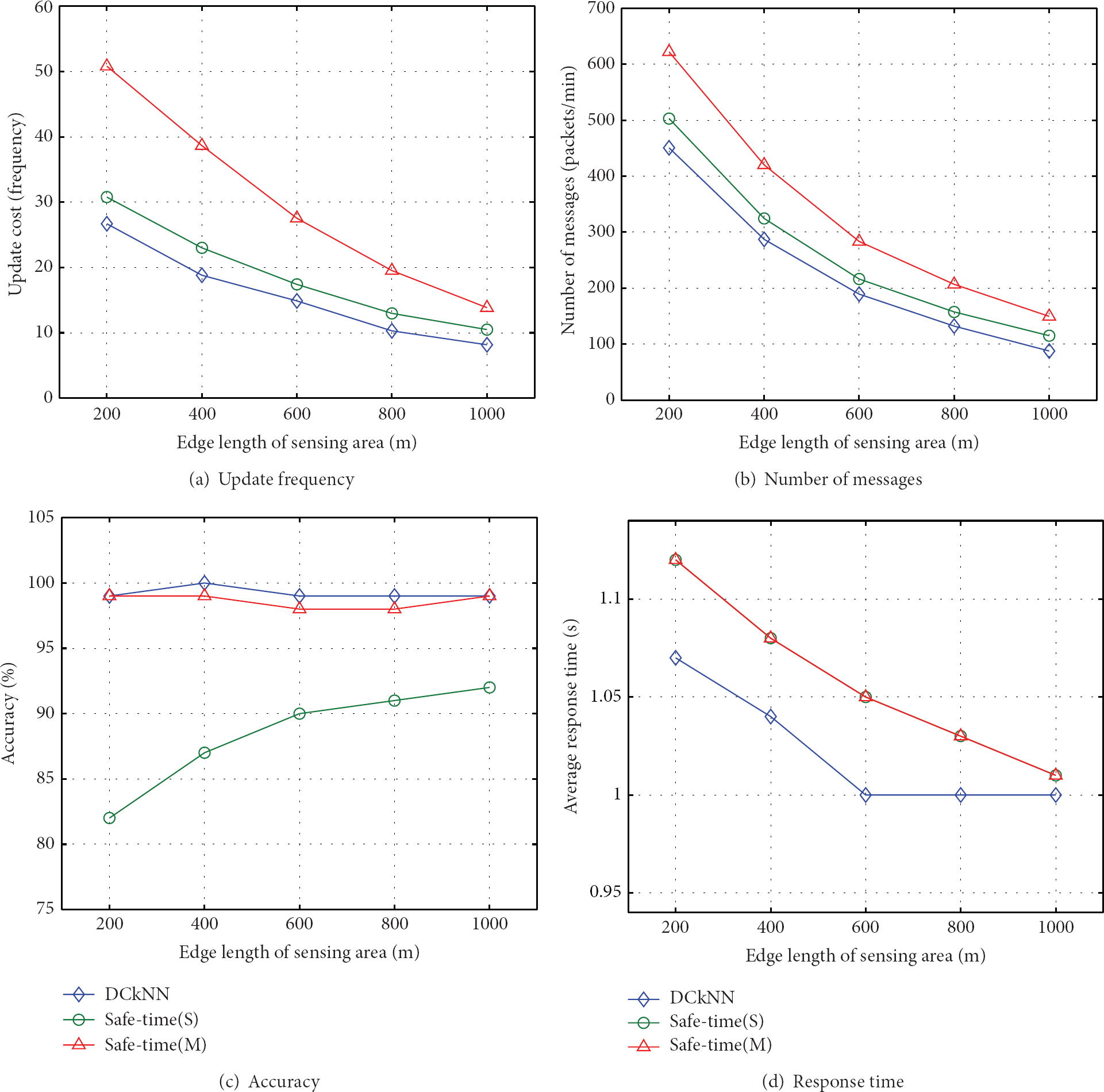
The effects of different sensing areas on (a) update frequency, (b) number of messages, (c) accuracy, and (d) response time.
To monitor the results, DCkNN only needs to check the related objects in the local Voronoi cell at the proper safe-time, thus reducing a lot of redundant update messages. Safe-time(S) and Safe-time(M) use the maximum speed of the objects to calculate the safe time, so the total number of transmitted messages of both approaches is more than that of DCkNN. Figure 13(b) shows that more than 30% of the total number of transmitted messages can be saved by DCkNN in comparison with Safe-time(M).
For the accuracy, since Safe-time(S) does not consider the query movement, the safe-time may be inaccurate. Furthermore, due to the mobility, when the density is high, the estimated results become more inaccurate. So, Safe-time(S) performs worst as shown in Figure 13(c). Safe-time(M) is revised from Safe-time(S) by considering the query movement and the safe-distance is less in average for guaranteeing better results. Hence Safe-time(M) has a better accuracy and almost the same as DCkNN. The accuracy of Safe-time(M) and DCkNN is almost about 100% correct and the gap may be caused by arithmetical errors in the experiments.
When the area becomes larger, the density becomes lower. So, the number of objects in each object's transmission range is fewer. Under such a circumstance, DCkNN uses less computation and the response time is shorter as shown in Figure 13(d). In contrast, the Safe-time(S) and the Safe-time(M) need to collect information before performing each new query and cause longer response time. Since Safe-time(M) and Safe-time(S) use the same method and procedure to handle the first query, the response time of these two methods will be almost the same.
6.2. Effects of Grid Size
In this simulation experiment set, we want to observe the update efficiency of each object in the third phase of DCkNN. Recall that we consider the grid-based and VD-base safe distances to derive a proper safe-time. In this experiment, DCkNN(G) uses grid-based safe distance to determine the safe time for the next update and DCkNN(V) uses VD-base safe distance to derive the safe time. The sensing area is fixed to 600*600 m2 and there are 30 data objects. We compare DCkNN(V) with DCkNN(G) by observing the impacts of different grid sizes. All the other settings have the similar trends in our experimental results. In Figure 14(a), the update frequency of the objects in DCkNN(G) is high when the grid size is 50*50 m2 and becomes less when the grid size decreases. Since the sensing area is 600*600 m2 and 30 objects are given, the average distance between an object and the boundary of a Voronoi cell is about 25 to 50 meters. With the setting of grid size 50*50 m2, the average distance obtained in DCkNN(G) is about 25 meters. Thus, the safe time of DCkNN(V) is longer. In general, as Figures 14(a) and 14(b) show, the update frequency of the objects and the number of messages, sent by the objects, decrease as the grid size increases.
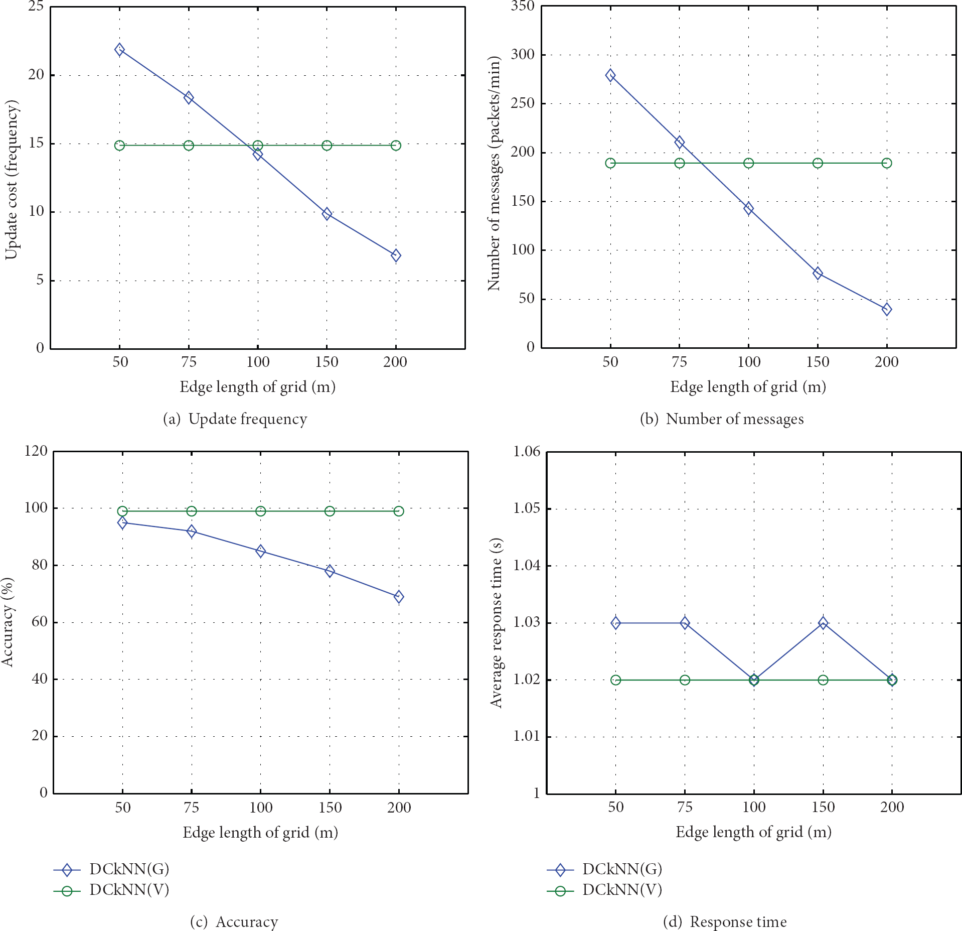
The comparisons of using grid-based and VD-base safe distances to derive the safe-time: (a) update frequency, (b) number of messages, (c) accuracy, and (d) response time.
When the grid size is large, the safe time becomes long and less number of updates are issued. Hence, the results become more inaccurate. As shown in Figure 14(c), when the grid sizes are 50*50 m2, 75*75 m2, 100*100 m2, and 150*150 m2, the corresponding accuracies are 95%, 92%, 85%, and 78%, respectively. While the grid size increases to 200*200 m2, the accuracy is significantly reduced to 69%, and the right answer thus can not be guaranteed. On the other hand, Figure 14(d) shows that the response times of DCkNN(G) and DCkNN(V) are not much different, because the size of grid is not the major factor to influence the complexity of obtaining information for the first query.
6.3. Number of Objects
In this subsection, we discuss the results as the number of data objects varies. The area in the presented experiment set is 600*600 (m2) with grid size of 50*50 (m2). As shown in Figure 15(a), when the number of objects increases, the number of updates in DCkNN is still relatively less than the ones in Safe-time(S) and Safe-time(M). If the number of objects increases, the number of replied messages per second to the central server in naïve will grow dramatically. With 20 to 60 objects, the number of replied messages to the server is from 1200 to 3600 (packets/min). By observing the results in Figures 15(b) and 15(c), as more objects are in the area, the number of messages increases for the other three methods and the accuracy reduces in Safe-time(S). These match the trends for different areas we discussed earlier due to the density. Similarly, the response time can be expected as shown in Figure 15(d) where the response time of DCkNN is still the shortest.
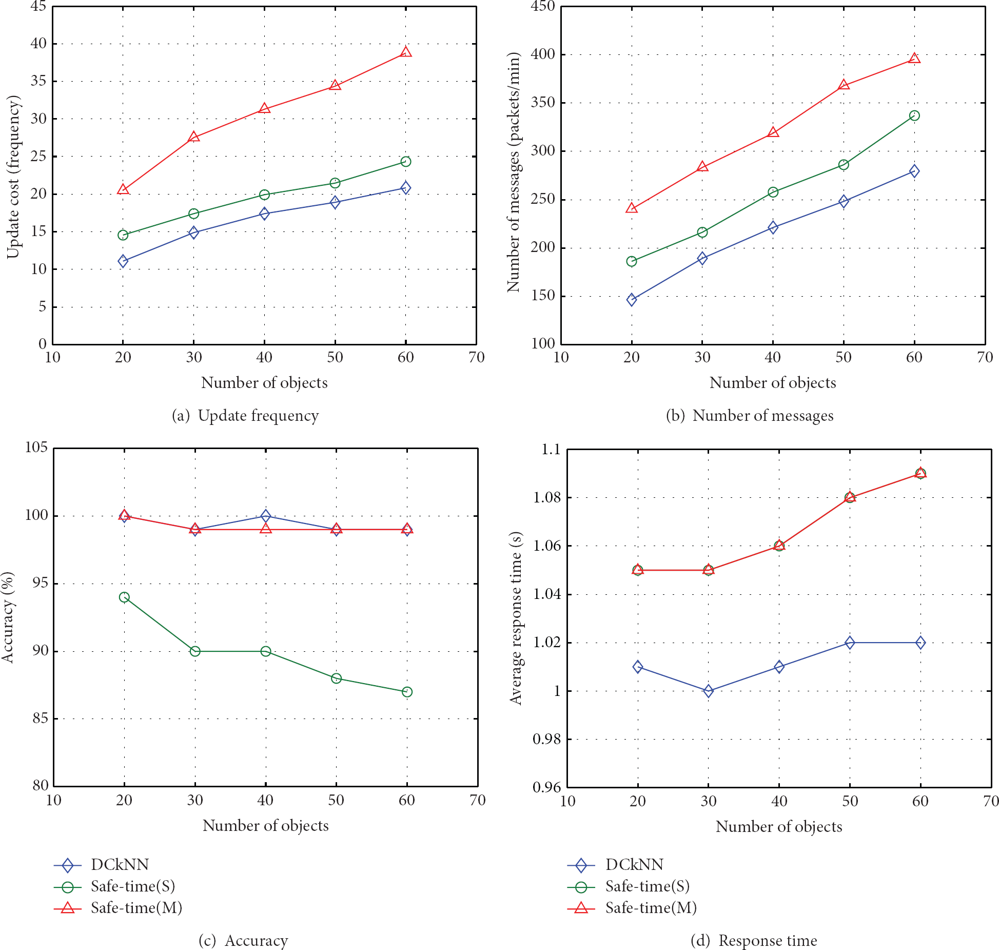
The effects of the number of objects on (a) update frequency, (b) number of messages, (c) accuracy, and (d) response time.
6.4. Different Values of k
It is obvious that the value of k affects the performance of query processing significantly. When the value of k becomes larger, the number of related objects required to be checked also increases. In other words, we need to spend more cost to find out which k objects are currently in the result for the CkNN query. Therefore, the changes in the value of k mainly affect the amount of data required for the first query and the update cost for maintaining the kth and the

The impacts of different values of k on (a) update frequency, (b) number of messages, (c) accuracy, and (d) response time.
Figure 16(c) presents the impact on the accuracy for different values of k. With a larger value of k, an object in Safe-time(S) will have a higher chance to derive the incorrect safe time, thus causing lower accuracy. When the value of k increases, the response time of all three methods will increase significantly, as shown in Figure 16(d). The reason is that all DCkNN, Safe-time(S), and Safe-time(M) need to search more objects and collect more information for answering the query when the value of k increases to a certain number. For DCkNN, DCkNN only needs to store local Voronoi diagram, where the information required is less than required in Safe-time(S) and Safe-time(M), so the response time of DCkNN is the shortest.
6.5. The Effect of Moving Objects
In this experiment set, we consider different percentages of moving objects in all the data objects. The default value is 20%, which means that if there is a total of 30 objects, then there are six moving objects. In Figures 17(a) and 17(b), as the percentage of moving objects increases, the overall number of updates required between the objects increases relatively and the change rate of answer to the DCkNN accelerates, thus increasing the update frequency of the query and the number of messages. However, DCkNN still keeps the best performance. Figure 17(c) shows the accuracy of the result for different percentage of moving objects. DCkNN and Safe-time(M) both have higher accuracy and Safe-time(S) is still the worst. The safe time of each object in Safe-time(S) is calculated using the maximum speed of the objects. Hence whether the object is moving or not does not directly result in the incorrectness of the answer collection. In fact, in Safe-time(S), one of the main reasons to affect the accuracy is the directions of moving objects. Last, as Figure 17(d) shows, the percentage of moving objects does not impact the response time too much.

The effects of the moving objects on (a) update frequency, (b) number of messages, (c) accuracy, and (d) response time.
6.6. Effects of Speed
If each object moves faster, the relative velocities between objects may also become faster. This will make the safe time shorter and the update frequency of each object and query increases. The safe time, used in Safe-time(S) and Safe-time(M), is directly affected by the maximum speed of objects and does not consider the direction of each object's movement and the speed of individual movement. No matter the objects move or not and move fast or slow, both of the above methods directly use the maximum speed of objects to calculate the safe time for updating. On the other hand, DCkNN considers the moving direction of objects and the proper safe-time for updates. In this experiment, the number of moving objects is 20% of all the objects. As Figure 18(a) shows, as the moving objects speed up, the update cost increases and DCkNN still performs best. As the speed increases, the safe-time in Safe-time(S) and the Safe-time(M) becomes much shorter due to a larger maximum speed among all the objects. The trend becomes even worse as the speed increases.
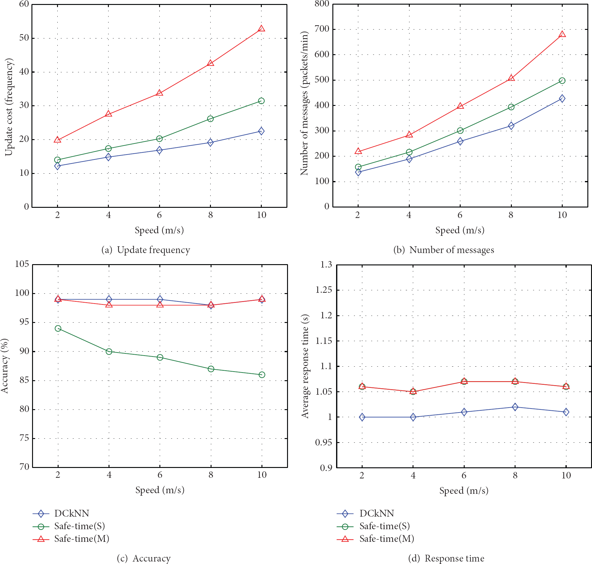
The impacts of speed on (a) update frequency, (b) number of messages, (c) accuracy, and (d) response time.
Figure 18(b) shows the trend about the number of transmitted messages when the speed is up. DCkNN still has the best performance on the number of messages. There are 427.81 messages sent in average, when the speed of object is 10 m/s. However, the Safe-time(M) needs 679.13 messages. The accuracy will not be effected as the speed changes for DCkNN and Safe-time(M) because both of them are designed or adapted for the moving objects and queries. Safe-time(S) will have more inaccurate results as the speed is high as shown in Figure 18(c). However, the response time does not have a significant impact on the response time for all the three methods. Figure 18(d) presents this trend.
7. Conclusions
In this paper, we propose a new approach, DCkNN, which uses the local Voronoi diagram and proper safe-time to effectively process the CkNN query in distributed and mobile environments, such as wireless sensor networks. The proper safe-time can be quickly derived by a simple formula. By comparing our proposed DCkNN with other existing approaches, Safe-time(S), DCkNN, can effectively improve search efficiency, reduce response time and the number of messages, and keep the accuracy of the result high. Additionally, DCkNN reduces more 30% of transmission messages than Safe-time(M) because the characteristics of the Voronoi diagram are used and each object's moving direction is considered instead of directly using the maximum speed of the objects as Safe-time method. The derived safe-time is more precise. As a result, DCkNN needs less update frequency, reduces a great number of messages transmitted, and yields more accurate results. In this work, simulation experiments are also performed. The experimental results validate the proposed DCkNN approach for the continuous k nearest neighbor query in distributed and mobile environments where all the data objects and query can move.
Footnotes
Acknowledgment
This work is partially supported by NSC under the Grant 98-2220-E-027-007, 100-2221-E-027-087-MY2, and 102-2221-E-027-088-.