
Abstract
Node localization technology is especially important to most applications of wireless sensor network. However, each mobile beacon needs to broadcast its current position many times, and locating all the nodes must take a long time in most of the localization algorithms. In order to solve these problems, we propose a novel range-free localization algorithm—localization with a mobile beacon based on compressive sensing (LMCS). LMCS makes use of compressive sensing (CS) to get the related degree of the sensor nodes and all the mobile beacon points. According to the related degree, the algorithm decides the weight value of each beacon point for the mass coordinate, and estimates the sensor node location. LMCS does not ask for all nodes hearing directly with beacon node, so it is more suitable for practical application than other localization algorithms. The simulation results show that compared with MAP schemes, LMCS has better localization performance, especially under irregularity of radio range and obstacle environment. Therefore, LMCS is a reliable, useful, and effective localization algorithm.
1. Introduction
With the development of technology, wireless sensor networks have been widely used for various applications, such as routing, monitoring, and tracking. A wireless sensor network is composed of a large number of cheap and energy limited sensor nodes, which are densely distributed in a field, and each sensor node can detect specific events in its sensing field. In wireless sensor networks, there are several important issues (e.g., localization, deployment, and coverage). However, localization is the most essential problem because the location information is the important premise for deployment, coverage, routing, monitoring, and tracking.
Many localization algorithms, broadly divided into two categories, have been proposed, including range-based schemes and range-free schemes. The range-based schemes are achieved by measuring the distance between two neighbor nodes [1–8]. For instance, the distance can be calculated based on the Received Signal Strength Indication (RSSI), Time of Arrival (TOA), Time Difference of Arrival (TDOA), or Angle of Arrival (AOA). The range-based location algorithms have high location precision common, but it require additional measuring equipment. Many range-free schemes have been proposed in [9–20].
Compared with the Nyquist sampling theorem, compressive sensing (CS) [21, 22] only needs fewer noisy measurements to recover the signal, which is sparse or compressible under a transform basis. CS can reconstruct exactly the original sparse signal with high probability by dealing with a minimization problem [23–25]. Many researchers [26–28] address target localization problem in WSNs using the theory of CS. In [26], a novel multiple target localization approach based on CS theory is proposed, and a preprocessing is introduced to enable the measurement matrix to meet Restricted Isometry Property (RIP) [22], so the performance can be guaranteed. In [27], Zhao and Xu propose a novel target localization algorithm based on Bayesian CS, and the algorithm can effectively save the energy of sensor node, but it may produce false targets. In [28], Zhang et al. propose a Greedy Matching Pursuit (GMP) algorithm to reconstruct the signal with a better resistance to noise compared with the traditional algorithm. However, these algorithms solve not only node localization, but also target localization by CS, and they all adopt RSSI to localization, so the performance of them will be affected by noise. In this paper, we use CS to realize node localization, and the algorithm proposed adopts the connectivity information, rather than RSS, which can avoid the influence of noise.
In this paper, a novel range-free localization approach, LMCS, is proposed. In LMCS, we only use the connectivity information to locate the positions of all sensor nodes. First, the mobile beacon periodically sends a message, and each sensor node gets the hop-count from the position, where the mobile beacon broadcasts the message. The mobile beacon obtains the connectivity information between all beacon points through the use of sensor nodes. Then, we utilize all connectivity information to compute the degree of correlation between the sensor node and all beacon points by CS. Finally, by the degree of correlation, we can get the locations of all sensor nodes.
The rest of the paper is organized as follows. Section 2 introduces the related works on localization in WSN. A brief of background on CS and Centroid are introduced in Section 3. We describe the detail of LMCS in the Section 4. The performance of LMCS is shown in Section 5. Finally, the conclusion is given in Section 6.
2. Related Work
Many algorithms have been proposed to solve the localization problem in the literature. Excellent surveys of the related studies can be found in [29]. The major localization studies are summarized in the section below.
2.1. Range-Based
The range-based schemes are achieved by measuring either node-to-node distances or angles to estimate locations. The typical range-based schemes include strategies based on RSSI, TOA, TDOA, and AOA. In [1], the RSSI is converted to distance information and then node's location is estimated by using the triangulation. Bergamo and Mazzini propose a triangulation strategy for the localization and analyze the effects of fading and sensor mobility on localization [2]. To estimate its possible locations, node uses the beacon advertisements received for ranging [3]. Niculescu and Nath compute comparative angles between neighboring nodes for angulations [4, 5].
2.2. Range-Free
Due to the sensor devices' hardware limitations, the range-free schemes are more economic than the range-based schemes. Centroid scheme is proposed by Bulusu et al. [9]. Centroid formula based on received beacons' locations is used to determine node's locations. The improved Centroid schemes are proposed in [10, 11]. Niculescu and Nath introduce DV-Hop approach to estimate node's locations by measuring hop-counts from each node to specific beacons [12]. The DV-Hop algorithm is improved by using RSSI technology in [13]. APIT scheme uses few beacons to locate each sensor node, but needs high density of beacons [14]. Tran and Nguyen propose LSVM algorithm, which applies SVM to locate sensor node [15].
2.3. Mobile Beacon
As beacons are powerful but expensive, it is very important to minimize the number of beacons, which is used to locate nodes' position. Assume few beacons can move and periodically broadcast their locations, in other words, many statistical beacons can be replaced by few mobile beacons. Therefore, many schemes are proposed by using a beacon or few beacons. Widely speaking, these schemes can also be divided into range-based and range-free.
A range-based localization mechanism combined with the RSSI technique is proposed in [6], sensor nodes' possible locations can be estimated by hearing a single mobile beacon. Sun and Guo's probabilistic localization algorithm based on a mobile beacon utilizes TOA technique for ranging and uses Centroid formula based on distance information to estimate nodes' location [7]. Xia and Chen present a localization scheme by using TDOA technique with mobile beacons, in which the nodes use trilateration to decide their locations [8].
The half arrival and departure overlap (HADO) is a range-free localization scheme proposed by Xiao et al., and it adopts arrival and departure constraint area to decide each node's location [16]. However, HADO has a strict requirement for the path of mobile beacons. In [17], antennas are introduced to estimate each node location, so mobile beacon needs to equip with four directional antennas. In Ssu's MAP localization algorithm, the information received from the mobile beacon is used to find two chords of a circle, and the senor node's location can be estimated by the center of the circle [18]. MAP + GC algorithm uses the intersecting area of two circles to decide the node's location within a possible sensing area by utilizing geometric constraints [19]. Liao et al. propose two enhanced MAP schemes—MAP − M and MAP − M&N, in these algorithms, if the centre and radii of two circles are known, two possible locations are obtained, and then the node's location can be ensured by beacon or neighbor node [20].
3. Compressive Sensing and Centroid
3.1. Compressive Sensing
Nyquist sampling theorem suggests that the sampling rate must be at least double the signal's bandwidth to reconstruct original signal exactly. However, for a large bandwidth signal, a high sampling rate causes too much sampling points, and increases the calculation of the subsequent signal processing. CS technology [21, 22] can solve this problem since it can greatly compress the sampling data to reduce computation. A brief introduction of CS is described below.
Suppose


However,
3.2. Centroid
Centroid lets the geometric center of all beacons within the sensor node communication range be sensor node's estimated position. The localization process can be described as follows: each beacon periodically broadcasts a beacon signal, which includes the ID and location information of the beacon, to the neighbor nodes. When the sensor node receive the number of the beacon signal from beacon node that exceeds the preset threshold in a period of time, the sensor node will let the geometric center of all beacons within the sensor node communication range be estimated position of the sensor node. Assume that there are N nodes

Then, the various improved algorithms have been proposed in [10, 11], and the weighted Centroid were presented that the weighted coefficient is gained through the RSSI between beacon and sensor node.
In this paper, we let the weighted Centroid of all beacon points be the estimated location of the sensor node. According to the correlation degree between the sensor node and all beacon points, the weighted coefficient for the Centriod will be obtained. LMCS is different from traditional Centriod, and it uses not only few one-hop beacon points, but also all beacon points in the location estimation process.
4. LMCS: Localization Algorithm with a Mobile Beacon Based on Compressive Sensing
4.1. Localization Algorithm Principle


The connectivity information between the jth sensor node and all k beacon points is shown as

In the same way, the measurement

Then, the position of the jth sensor node

4.2. Algorithm and Protocol
The algorithm for the sensor node localization mainly includes three parts. First, calculate the correlation coefficient between the sensor node and all beacon points. Second, utilize the correlation coefficient ensured above to compute the weighted value between the sensor node and all beacon points. Finally, estimate the location of the sensor node. The process of LMCS is described as follows.
Algorithm (estimate the location of the sensor node Input: the measurement Output: the position The process for the sensor node localization is as follows calculate the correlation coefficients between sensor node use the correlation coefficients obtained above to compute the weighted values both them by (13); estimate the position
According to the principle description, the key to locate a sensor node is the related degree between the sensor node and all beacon points. Then the localization Protocol of sensor nodes can be divided into three stages.
Stage 1: Data Collection. The mobile beacon which reaches the ith beacon point should send a HELLO message
Stage 2: Advertisement. The mobile beacon lets the connectivity information
Stage 3: Localization. Each sensor node starts this stage after receiving the sample dictionary A from the advertisement stage. First, each sensor node compresses the hop-count information
4.3. Algorithm Analysis
Figure 1 shows how to linearly decompose one sensor node by all beacon points. The square represents the sensor node, and circular and star express all beacon points with zero correlation coefficients and nonzero correlation coefficients, respectively. When the star is greater, the coefficient is greater. As shown in Figure 1, the closer the position of the beacon point in geometry is, the larger the correlation coefficient may be, but the further away the position of the beacon point is, the smaller the correlation coefficient must be, and even close to 0, which trends coincide well with the reality. We can also find
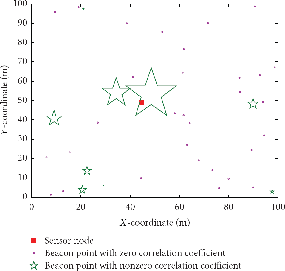
The schematic of the correlation coefficients.
4.4. Error Analysis
We analyze the LMCS error bound under the effect of the CS error in theoretical as follows.
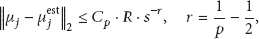
Lemma 1.
One fix an orthogonal basis

This means that p controls the speed of the decay: the smaller the p, the faster the decay.
Theorem 2.
Suppose all the coefficients

Then, the error of the related degree between the sensor node and all beacon points can be obtained as
Assume the jth sensor node is exact linearly expressed by all beacon points, then the real location can expressed as

According to (12), the estimate location of the jth sensor node can be obtained as

According to (17) and (18), we can get the localization error E as follows:
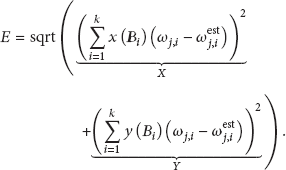
Let
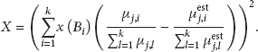
Because

Based on the same reason, the inner summation Y can be expressed as

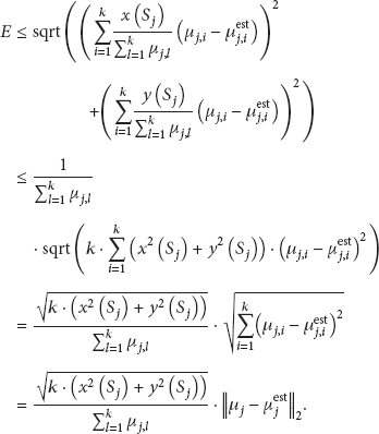
According to above deduction and (16), we can describe the localization error E as follows:

5. Simulation Study and Analysis
To compare the performance of MAP + GC [19], MAP – M [20], and MAP − M&N [20] with LMCS, we discuss the performance of four algorithms under ideal environment (Figure 2(a)) and obstacle environment (Figure 2(b): assume that there are four 10 m × 20 m obstacles that existed in the sensing field), and analyze the radio range, GPS error, radio irregularity, and the velocity of mobile beacon to impact on the performance of four algorithms. We also discuss the effect of compression ratio and radio time on the performance of LMCS.

Simulation environment.
Take one network with 1,000 sensor nodes for example, suppose all nodes locate in a 100 m × 100 m area, and their locations obey uniform random distribution. We assume that the mobile beacon and all the sensor nodes have the same communication range being 20 m, the mobile beacon is assumed to move straight at a velocity of 20 m/s and the mobile beacon path follow the random waypoint (RWP) model [31]. In three MAP algorithms, the mobile beacon broadcasts a message every 0.1 sec, and 10000 times; in LMCS, the mobile beacon broadcasts a message every 1 sec, and 800 times, the measurement matrix
5.1. Ideal Environment
Figure 3 shows each node's location error in ideal environment. In Figures 3(b), 3(c), and 3(d), the red circles represent the nodes, which are not located. We can see, roughly, that most of the location errors have no more than 5 m in LMCS, but many location errors are large in three MAP schemes. It can be also found that the maximum location error of LMCS is far smaller than that of MAP + GC, MAP − M, and MAP − M&N. As the beacon points exist, there is improper selection in MAP + GC, MAP − M, and MAP − M&N, which will cause a large location error. Although the mobile beacon broadcasts 10000 times, some sensor nodes still cannot be located for MAP + GC, MAP − M, and MAP − M&N. But this problem is nonexistent in LMCS. As LMCS uses the connectivity information to localize nodes, and no matter how many time the radio is, all nodes can be localized. However, for the other three schemes, the radio time will affect the number of nodes localized. To localize all nodes, these three schemes must have high radio time. Certainly, the localization accuracy of LMCS will be affected by the radio time.

The location error of each sensor node.
We make 120 times Monte Carlo experiments to obtain the average location error of the four schemes under an ideal environment, which is shown in Table 1. The average location error of LMCS is smaller than that of MAP + GC, MAP − M, and MAP − M&N. Therefore, LMCS is a better choice for localization than MAP + GC, MAP − M, and MAP − M&N.
The localization performance comparison.

5.2. Obstacle Environment
Table 2 illustrates the localization performance comparison under obstacle environment for the four methods. We can see that the average location error of LMCS is smaller than that of MAP + GC, MAP − M, and MAP − M&N; in other words, the localization performance of LMCS is much better than MAP + GC, MAP − M, and MAP − M&N.
The localization performance comparison.
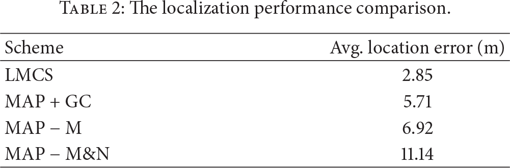
Compared with Tables 1 and 2, we can find the localization performance of four methods under obstacle environment is worse than under ideal environment, and the influence of environment on LMCS is much less than MAP + GC, MAP − M, and MAP − M&N. Due to existing obstacles, the choice of beacon point is more prone to errors in MAP + GC, MAP − M, and MAP − M&N, and the localization performance of MAP + GC, MAP − M, and MAP − M&N is much worse. However, as obstacles only have little impact on the connectivity information, the performance of LMCS will not get worse.
5.3. Impact of GPS Error
All GPS receivers have localization error in real environments, which include three basic location errors, that is, single-point positioning error, differential positioning error, and carrier positioning error [32]. The simulations assume GPS errors based on a normal distribution. Applying the carrier positioning error, the mean GPS errors are specified as 0, 0.1, 0.2, 0.3, 0.4, 0.5, 0.6, 0.7, 0.8, 0.9, and 1 meter, respectively, with a standard deviation of 0.05 meters.
Figure 4 illustrates the variation of the localization error with the GPS error for the four methods. In general, with the increase of the GPS errors, the location errors of the four schemes are increased with a slow trend, in other words, while GPS errors are small, the impact of which is not very obvious for localization accuracy.

Relationship between localization performance and GPS error.
5.4. Impact of Radio Range
Figure 5 shows the variation of the location error as the radio range for the four schemes. It can be seen that, with the increase of the radio range, the location errors of the four schemes are increased. And yet, the impact of radio range on MAP + GC, MAP − M, and MAP − M&N is more than LMCS.

Relationship between localization performance and radio range.
5.5. Impact of Radio Irregularity
As the radio range of node is irregular in practical environment, the influence of degree of irregularity (DOI) is discussed in this section. DOI is defined as the maximum radio range variation per unit degree change in the direction of radio propagation as
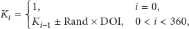
Figure 6 describes the average location error of these four schemes under different DOI. As shown, the average location errors of MAP + GC, MAP − M, and MAP − M&N schemes are increased with the increase of DOI, in other words, DOI has an evident influence on these three schemes. However, the average location error of LMCS remains a constant. Namely, DOI has a slight influence on LMCS. This is because MAP + GC, MAP − M, and MAP − M&N schemes make use of the irregular radio range to estimate the location of the node, but LMCS use the connectivity information, and DOI has little effect on the connectivity information.

Relationship between localization performance and DOI.
5.6. Impact of the Velocity of Mobile Beacon
Figure 7 shows the variation of the location error as the velocity of mobile beacon for the four schemes. It can be seen that, with the increase of the velocity, the location errors of LMCS scheme is almost a constant value, but the location errors of MAP + GC, MAP − M, and MAP − M&N schemes are increased. Because the velocity is different, beacon distance which affects the performance of MAP + GC, MAP − M, and MAP − M&N schemes is also different. But in LMCS, since the number of beacon points is the same, the completeness of the sampling dictionary remains almost unchanged and the performance remains. Therefore, the velocity of mobile beacon has obvious influence on MAP + GC, MAP − M, and MAP − M&N, but almost no influence on LMCS.

Relationship between localization performance and the velocity of mobile beacon.
Table 3 illustrates the number of sensor nodes localized comparison under different the velocity of mobile beacon for the four methods. As it can be seen, the number of sensor nodes localized is increased with the increase of the velocity for MAP + GC, MAP − M, and MAP − M&N schemes, but LMCS scheme has always localized all nodes. In Figure 7, we can see that the performance of MAP + GC is slightly better than that of LMCS while the velocity is 10 m/s, however, according to Table 3, our scheme can localize all node while the mobile beacon just broadcasts 800 times, but MAP + GC only localizes 886 nodes while the mobile beacon broadcasts 10000 times. Besides, we can increase the broadcasting time to improve the performance of LMCS scheme.
The number of sensor nodes localized.

5.7. Impact of Compression Ratio
The average location error as the function of compression ratio

Relationship between localization performance and compression ratio.
5.8. Impact of Radio Time
Figure 9 shows the average location error as the function of radio time in LMCS. It can be seen that the localization error of sensor nodes reduces with the increase of radio time. Since the sampling dictionary becomes more complete while radio time is more, then sensor nodes can be more accurately expressed. Therefore, the localization performance becomes better.
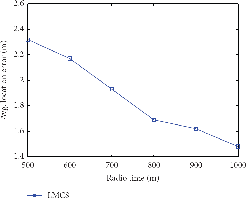
Relationship between localization performance and radio time.
6. Conclusion
A novel range-free localization algorithm—LMCS is proposed in this paper. LMCS makes use of CS to excavate the degree of correlation between sensor nodes and beacon points, and then weighted Centroid to realize node localization. Simulation studies confirm that, compared with MAP + GC, MAP − M, and MAP − M&N, LMCS has lower average location error. What is more, as LMCS adopts the connectivity information to localize each node, the obstacles and DOI have little effect on LMCS, but they have great effect on these three MAP algorithms. Therefore, LMCS is more suitable for practical application than MAP algorithms. In addition, LMCS can completely locate all nodes with few beacon points, but MAP algorithms cannot ensure to completely locate all nodes even with huge beacon points. Above all, LMCS is a reliable, effective, and useful range-free localization algorithm and more suitable for practical application. However, LMCS also has few shortcomings, such that it needs sensor node to obtain the connectivity information, and it consumes energy of sensor node.
Footnotes
Acknowledgments
This study is supported by the National Natural Science Foundation of China (61077079), the Ph.D. Programs Foundation of the Ministry of Education of China (20102304110013), and the Fundamental Research Funds for the Central Universities (HEUCF1208).