Variational Inference of Kalman Filter and Its Application in Wireless Sensor Networks

Abstract

An improved Kalman filter algorithm by using variational inference (VIKF) is proposed. With variational method, the joint posterior distribution of the states is approximately decomposed into several relatively independent posterior distributions. To avoid the difficulty of high-dimensional integrals, these independent posterior distributions are solved by using Kullback-Leibler divergence. The variational inference of Kalman filter includes two steps, the predict step and the update step, and an iterative process is included in the update step to get the optimized solutions of the posterior distribution. To verify the effectiveness of the proposed algorithm, VIKF is applied to the state estimation of discrete linear state space and the tracking problems in wireless sensor networks. Simulation results show that the variational approximation is effective and reliable for the linear state space, especially for the case with time-varying non-Gaussian noise.

1. Introduction

The Kalman filter (KF), also known as linear quadratic estimation (LQE), is one of the most used linear state estimation methods and has numerous applications [1], which include guidance, navigation, and control of vehicles [2–5]. Kalman filter is also widely applied in time series analysis in fields such as signal processing and econometrics [6, 7]. Other nonlinear methods, such as Extension-Kalman filter (EKF) [2] and unscented Kalman filter (UKF) [8], also use the Kalman filter to fix problems, combined with the linearization of nonlinear functions or the approximation of the probability density distribution, respectively. Practical implementation of the Kalman Filter is often difficult due to the inability of getting a good estimate of the noise covariance matrices. Extensive researches have been carried out in this field to estimate these covariances from data, such as the autocovariance least-squares (ALS) [9, 10], the modified Bryson-Frazier smoother [11], and the minimum-variance smoother [12, 13].

Variational inference for the Kalman filter in linear state space model was also considered in several literatures [14–16]. However, the authors in [14] just used the limited memory BFGS method to decrease the computational burden, both factorization and Kullback-Leibler (KL) divergence [15] (the expectation of joint distribution with holding some variable distribution as constant) were not considered. Works in [16] indeed applied the variational approximation, and got the posterior distributions of the state variables and the measurement noise. However, in the update step of the Variational Bayesian approximation Adaptive Kalman Filter (VBAKF), the initial values of states or variances were used in all iterative steps; thus, the iterations would quickly reach “steady states.” Sometimes, the maximum number of the iterations is only 2 in the algorithm. That is to say that there are only two effective iterative loops performed in the update step of the Kalman filter, therefore, the performance of this algorithm is not good in such cases as the non-Gaussian and high-dimensional linear state space models. In this paper, we rederive the parameter expressions for the Kalman filter by using variational inference method (we call it VIKF in this paper), which can really form an iterative process for the update step of the Kalman filter.

Location and tracking are the keys in variety WSN applications [17–19], where the Kalman filter and its extension algorithms are widely used. In this paper, we will also consider the application of VIKF for WSN tracking problems, especially with time-varying and non-Gaussian noises.

This paper is organized as follows. We firstly introduce the linear state space model, then the derivation of Kalman filter by using variational inference (VIKF) follows, and the iterative process of VIKF is presented. In simulation section, the effectiveness of our proposed method will be demonstrated by examples. Finally, we will compare VIKF with standard KF and VBAKF in the cases of high-dimensional discrete state spaces, and the tracking in WSN with non-Gaussian noise.

2. The Linear State Space Model

Linear state space models are a widely used class of models for control, economics, and so on. The most general state-space representation of a discrete-time linear system with K samples, n state variables, and m outputs is written in the following form:

$$\begin{array}{cc}& {\mathbf{X}}_k={\mathbf{M}}_k{\mathbf{X}}_{k-\mathrm{1}}+{\mathbf{\epsilon }}_k^x,\end{array}$$

(1)

$$\begin{array}{cc}& {\mathbf{Y}}_k={\mathbf{N}}_k{\mathbf{X}}_k+{\mathbf{\epsilon }}_k^y,\end{array}$$

(2)

where ${\mathbf{X}}_k$ is an $n\times \mathrm{1}$ state vector of the system at time k, $k=\mathrm{1,2},\dots ,K$ . ${\mathbf{M}}_k$ is the state transition matrix at time k. ${\mathbf{\epsilon }}_k^x$ is the corresponding prediction error vector of ${\mathbf{X}}_k$ , ${\mathbf{\epsilon }}_k^x$ ~ $N(\mathrm{0},{\mathbf{Q}}_k)$ . ${\mathbf{\epsilon }}_k^x$ is assumed to be independent and identically distributed (i.d.d), so ${\mathbf{Q}}_k$ is a diagonal matrix. ${\mathbf{Y}}_k$ is the observation vector, and we assume that there are m observations, so ${\mathbf{N}}_k$ is an $m\times n$ linear observation operator matrix. ${\mathbf{\epsilon }}_k^y$ is an $m\times \mathrm{1}$ observation error vector and assumed to be i.d.d; therefore, ${\mathbf{\epsilon }}_k^y~N(\mathrm{0},{\mathrm{\Gamma }}_k)$ , ${\mathrm{\Gamma }}_k=\mathrm{diag}({\sigma }_{k,\mathrm{1}}^{\mathrm{2}},\dots ,{\sigma }_{k,m}^{\mathrm{2}})$ . Time is indexed by k.

In general, we assume that the initial state has a Gaussian prior distribution ${\mathbf{X}}_{\mathrm{0}}$ ~ $N({\mathit{\mu }}_{\mathrm{0}},{\mathbf{P}}_{\mathrm{0}})$ , and ${\mathbf{M}}_k$ , ${\mathbf{Q}}_k$ , ${\mathbf{N}}_k$ , ${\mathit{\mu }}_{\mathrm{0}}$ , and ${\mathbf{P}}_{\mathrm{0}}$ are all known. In tracking problems, ${\mathbf{X}}_k$ includes the information of positions and speeds of the moving target, ${\mathbf{X}}_k={[p_x,p_y,s_x,s_y]}^T$ , where $(p_x,p_y)$ is the two-dimensional coordinate positions and $(s_x,s_y)$ is the two-dimensional speeds.

3. Variational Inference for the Linear Space Model

Variational inference techniques have been extensively studied to solve problems in various fields [20–23]. There are two steps in the optimization for the standard Kalman filter [24]. The first step is to predict the state ${\mathbf{X}}_k$ and ${\mathrm{\Gamma }}_k$ from the last state ${\mathbf{X}}_{k-1}$ and the observations ${\mathbf{Y}}_{\mathrm{1}:k-\mathrm{1}}$ . The second step is to update ${\mathbf{X}}_k$ and ${\mathrm{\Gamma }}_k$ using information from new observations ${\mathbf{Y}}_k$ .

3.1. Predict Step

This step calculates ${\mathbf{X}}_k$ and ${\mathrm{\Gamma }}_k$ from ${\mathbf{Y}}_{\mathrm{1}:k-\mathrm{1}}$ . Here we assume that $p({\mathbf{X}}_k,{\mathrm{\Gamma }}_k\mid {\mathbf{Y}}_{\mathrm{1}:k-\mathrm{1}})$ can be decomposed as

$$\begin{array}{cc}& p\left({\mathbf{X}}_k,{\mathrm{\Gamma }}_k\mid {\mathbf{Y}}_{\mathrm{1}:k-\mathrm{1}}\right)=p\left({\mathbf{X}}_k\mid {\mathbf{Y}}_{\mathrm{1}:k-\mathrm{1}}\right)p\left({\mathrm{\Gamma }}_k\mid {\mathbf{Y}}_{\mathrm{1}:k-\mathrm{1}}\right).\end{array}$$

(3)

According to (1), we know that $p({\mathbf{X}}_k\mid {\mathbf{Y}}_{\mathrm{1}:k-\mathrm{1}})$ is a Gaussian distribution:

$$\begin{array}{cc}& p\left({\mathbf{X}}_k\mid {\mathbf{Y}}_{\mathrm{1}:k-\mathrm{1}}\right)~N({\mathit{\mu }}_k^{\prime },{\mathbf{P}}_k^{\prime })\end{array}$$

(4)

with

$$\begin{array}{cc}& {\mathit{\mu }}_k^{\prime }={\mathbf{M}}_k{\mathit{\mu }}_{k-\mathrm{1}},\\ {\mathbf{P}}_k^{\prime }={\mathbf{M}}_k{\mathbf{P}}_{k-\mathrm{1}}{\mathbf{M}}_k^T+{\mathbf{Q}}_k,\end{array}$$

(5)

where ${\mathbf{P}}_{k-\mathrm{1}}$ is the variance of the distribution of last state ${\mathbf{X}}_{k-\mathrm{1}}$ .

$p({\mathrm{\Gamma }}_k\mid {\mathbf{Y}}_{\mathrm{1}:k-\mathrm{1}})$ is the posterior variance of observation errors. We can assume that $p({\mathrm{\Gamma }}_k\mid {\mathbf{Y}}_{\mathrm{1}:k-\mathrm{1}})$ equals $p({\mathrm{\Gamma }}_{k-\mathrm{1}}\mid {\mathbf{Y}}_{\mathrm{1}:k-\mathrm{1}})$ temporarily in the prediction step, and it will be updated in the update step. We also assume that this posterior distribution is an inverse-Gamma distribution (also called Wald distribution). The inverse-Gamma distribution is often used in Bayesian inference, where the distribution arises as the marginal posterior distribution for the unknown variance of a normal distribution.

$p({\mathrm{\Gamma }}_k\mid {\mathbf{Y}}_{\mathrm{1}:k-\mathrm{1}})$ can be decomposed as

$$\begin{array}{cc}& p\left({\mathrm{\Gamma }}_k\mid {\mathbf{Y}}_{\mathrm{1}:k-\mathrm{1}}\right)={\displaystyle \prod }_{i=\mathrm{1}}^m\text{IG}({\alpha }_{k,i}^{\prime },{\beta }_{k,i}^{\prime }),\end{array}$$

(6)

where ${\alpha }_{k,i}^{\prime }$ , ${\beta }_{k,i}^{\prime }$ are the shape and scale parameters of inverse Gamma distribution $\text{IG}(·)$ , and set

$$\begin{array}{cc}& {\alpha }_{k,i}^{\prime }={\alpha }_{k-\mathrm{1},i},\\ {\beta }_{k,i}^{\prime }={\beta }_{k-\mathrm{1},i}.\end{array}$$

(7)

3.2. Update Step

This step updates ${\mathbf{X}}_k$ and ${\mathrm{\Gamma }}_k$ based on the new observation ${\mathbf{Y}}_k$ . According to the Bayes' rule,

$$\begin{array}{cc}& p\left({\mathbf{X}}_k,{\mathrm{\Gamma }}_k\mid {\mathbf{Y}}_{\mathrm{1}:k}\right)\propto p\left({\mathbf{Y}}_k,{\mathbf{X}}_k,{\mathrm{\Gamma }}_k\mid {\mathbf{Y}}_{\mathrm{1}:k-\mathrm{1}}\right).\end{array}$$

(8)

We assume that $p({\mathbf{X}}_k,{\mathrm{\Gamma }}_k\mid {\mathbf{Y}}_{\mathrm{1}:k})$ can be factored as

$$\begin{array}{cc}& p\left({\mathbf{X}}_k,{\mathrm{\Gamma }}_k\mid {\mathbf{Y}}_{\mathrm{1}:k}\right)=q\left({\mathbf{X}}_k\right)q\left({\mathrm{\Gamma }}_k\right).\end{array}$$

(9)

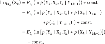
The variational method gets the approximation of each component by minimizing the Kullback-Leibler (KL) divergence between the estimated value and the true joint posterior. Each component can be obtained by performing the expectation operation to the joint distribution with respect to all other unknown parameters. So we have

$$\begin{array}{cc}& \ln q_{{\mathbf{X}}_k}\left({\mathbf{X}}_k\right)=E_{{\mathrm{\Gamma }}_k}\left(\ln p\left({\mathbf{Y}}_k,{\mathbf{X}}_k,{\mathrm{\Gamma }}_k\mid {\mathbf{Y}}_{\mathrm{1}:k-\mathrm{1}}\right)\right)+\text{const}.,\end{array}$$

(10)

$$\begin{array}{cc}& \ln q_{{\mathrm{\Gamma }}_k}\left({\mathrm{\Gamma }}_k\right)=E_{{\mathbf{X}}_k}\left(\ln p\left({\mathbf{Y}}_k,{\mathbf{X}}_k,{\mathrm{\Gamma }}_k\mid {\mathbf{Y}}_{\mathrm{1}:k-\mathrm{1}}\right)\right)+\text{const}.\end{array}$$

(11)

According to the known priori, we calculate (10):

$$\begin{array}{ll}\ln q_{{\mathbf{X}}_k}\left({\mathbf{X}}_k\right)& =E_{{\mathrm{\Gamma }}_k}\left(\ln p\left({\mathbf{Y}}_k,{\mathbf{X}}_k,{\mathrm{\Gamma }}_k\mid {\mathbf{Y}}_{\mathrm{1}:k-\mathrm{1}}\right)\right)+\text{const}.\\ & =E_{{\mathrm{\Gamma }}_k}(\ln [p\left({\mathbf{Y}}_k\mid {\mathbf{X}}_k,{\mathrm{\Gamma }}_k\right)*p\left({\mathbf{X}}_k\mid {\mathbf{Y}}_{\mathrm{1}:k-\mathrm{1}}\right)\\ & *p\left({\mathrm{\Gamma }}_k\mid {\mathbf{Y}}_{\mathrm{1}:k-\mathrm{1}}\right)\left]\right)+\text{const}.\\ & =E_{{\mathrm{\Gamma }}_k}\left(\ln \left[p\left({\mathbf{Y}}_k\mid {\mathbf{X}}_k,{\mathrm{\Gamma }}_k\right)*p\left({\mathbf{X}}_k\mid {\mathbf{Y}}_{\mathrm{1}:k-\mathrm{1}}\right)\right]\right)\\ & +\text{const}.,\end{array}$$

(12)

where $E_{{\mathrm{\Gamma }}_k}(\ln p({\mathrm{\Gamma }}_k\mid {\mathbf{Y}}_{\mathrm{1}:k-\mathrm{1}}))$ is a constant In (12), $p({\mathbf{Y}}_k\mid {\mathbf{X}}_k,{\mathrm{\Gamma }}_k)$ is a Gaussian distribution (see (2)), so we have

$$\begin{array}{cc}& p\left({\mathbf{Y}}_k\mid {\mathbf{X}}_k,{\mathrm{\Gamma }}_k\right)~N\left({\mathbf{Y}}_k-{\mathbf{N}}_k{\mathbf{X}}_k,{\mathrm{\Gamma }}_k\right).\end{array}$$

(13)

From the predict step, we know that $p({\mathbf{X}}_k\mid {\mathbf{Y}}_{\mathrm{1}:k-\mathrm{1}})$ is also a Gaussian distribution $N({\mathit{\mu }}_k^{\prime },{\mathbf{P}}_k^{\prime })$ (see (4) and (5)). The product of two Gaussian functions is still a Gaussian, so

$$\begin{array}{cc}& q_{{\mathbf{X}}_k}\left({\mathbf{X}}_k\right)=N\left({\mathbf{X}}_k\mid {\mathit{\mu }}_k,{\mathbf{P}}_k\right).\end{array}$$

(14)

Based on (4) and (13), we get the analytical expression of ${\mathit{\mu }}_k$ and ${\mathbf{P}}_k$ , and because variational method usually requires an iterative process to achieve convergence, so we expressed them as

$$\begin{array}{cc}& {\mathit{\mu }}_k^{\left(s+\mathrm{1}\right)}={\mathit{\mu }}_k^{\left(s\right)}+{\mathbf{P}}_k^{\left(s\right)}{\mathbf{N}}_k^T{\left({\mathbf{N}}_k{\left({\mathbf{P}}_k^{\left(s\right)}\right)}^{-\mathrm{1}}{\mathbf{N}}_k^T+{\mathrm{\Gamma }}^{\prime }\right)}^{-\mathrm{1}}\left({\mathbf{Y}}_k-{\mathbf{N}}_k{\mathit{\mu }}_k^{\left(s\right)}\right),\end{array}$$

(15)

$$\begin{array}{cc}& {\mathbf{P}}_k^{\left(s+\mathrm{1}\right)}={\mathbf{P}}_k^{\left(s\right)}-{\mathbf{P}}_k^{\left(s\right)}{\mathbf{N}}_k^T{\left({\mathbf{N}}_k{\left({\mathbf{P}}_k^{\left(s\right)}\right)}^{-\mathrm{1}}{\mathbf{N}}_k^T+{\mathrm{\Gamma }}^{\prime }\right)}^{-\mathrm{1}}{\mathbf{N}}_k{\mathbf{P}}_k^{\left(s\right)},\end{array}$$

(16)

where the superscript $(s)$ means the $s\text{th}$ iteration, ${\mathrm{\Gamma }}^{\prime }$ = $\mathrm{diag}({\beta }_{k,\mathrm{1}}/{\alpha }_{k,\mathrm{1}},\dots ,{\beta }_{k,m}/{\alpha }_{k,m})$ , ${\beta }_{k,i}$ , ${\alpha }_{k,i}$ , $i=\mathrm{1},\dots ,m$ will be computed lately. At the beginning of the iteration, we use the results of the predict step, set ${\mathit{\mu }}_k^{(\mathrm{0})}={\mathit{\mu }}_k^{\prime }$ , ${\mathbf{P}}_k^{(\mathrm{0})}={\mathbf{P}}_k^{\prime }$ .

Similar results also appeared in [16] and the algorithm there was called VBAKF. In the iteration process, VBAKF computes ${\mathit{\mu }}_k^{(s+\mathrm{1})}$ and ${\mathbf{P}}_k^{(s+\mathrm{1})}$ with ${\mathit{\mu }}_k^{(\mathrm{0})}$ and ${\mathbf{P}}_k^{(\mathrm{0})}$ , not ${\mathit{\mu }}_k^{(s)}$ and ${\mathbf{P}}_k^{(s)}$ ; therefore, VBAKF cannot form sufficient iteration during the update process. The maximum number of effective iterations of VBAKF is small, sometimes even only 2, so the performance cannot achieve the optimal solution of the variational method.

Similarly, we calculate $\ln q_{{\mathrm{\Gamma }}_k}({\mathrm{\Gamma }}_k)=E_{{\mathbf{X}}_k}(\ln p({\mathbf{Y}}_k,{\mathbf{X}}_k,{\mathrm{\Gamma }}_k\mid {\mathbf{Y}}_{\mathrm{1}:k}))+\text{const}$ . as

$$\begin{array}{l}\ln q_{{\mathrm{\Gamma }}_k}\left({\mathrm{\Gamma }}_k\right)=E_{{\mathbf{X}}_k}\left(\ln p\left({\mathbf{Y}}_k,{\mathbf{X}}_k,{\mathrm{\Gamma }}_k\mid {\mathbf{Y}}_{\mathrm{1}:k}\right)\right)+\text{const}.\\ \hspace{1em}\hspace{1em}\hspace{1em}=E_{{\mathbf{X}}_k}(\ln [p\left({\mathbf{Y}}_k\mid {\mathbf{X}}_k,{\mathrm{\Gamma }}_k\right)*p\left({\mathbf{X}}_k\mid {\mathbf{Y}}_{\mathrm{1}:k-\mathrm{1}}\right)\\ \hspace{1em}\hspace{1em}\hspace{1em}\hspace{1em}\hspace{1em}\hspace{1em}*p\left({\mathrm{\Gamma }}_k\mid {\mathbf{Y}}_{\mathrm{1}:k-\mathrm{1}}\right)])+\text{const}.\\ \hspace{1em}\hspace{1em}\hspace{1em}=E_{{\mathbf{X}}_k}\left(\ln \left[p\left({\mathbf{Y}}_k\mid {\mathbf{X}}_k,{\mathrm{\Gamma }}_k\right)*p\left({\mathrm{\Gamma }}_k\mid {\mathbf{Y}}_{\mathrm{1}:k-\mathrm{1}}\right)\right]\right)\\ \hspace{1em}\hspace{1em}\hspace{1em}\hspace{0.17em}+\text{const}.\end{array}$$

(17)

Based on the known conditions, we know that $q_{{\mathrm{\Gamma }}_k}({\mathrm{\Gamma }}_k)$ is still a Wald distribution, and can be expressed as

$$\begin{array}{cc}& Q_{{\mathrm{\Gamma }}_k}\left({\mathrm{\Gamma }}_k\right)={\displaystyle \prod }_{i=\mathrm{1}}^m\text{IG}\left({\sigma }_{k,i}^{\mathrm{2}}\mid {\alpha }_{k,i},{\beta }_{k,i}\right).\end{array}$$

(18)

In the iterations, parameters are calculated as follows:

$$\begin{array}{cc}& {\alpha }_{k,i}^{\left(s+\mathrm{1}\right)}=\frac{\mathrm{1}}{\mathrm{2}}+{\alpha }_{k,i}^{\left(s\right)},\end{array}$$

(19)

$$\begin{array}{cc}& {\beta }_{k,i}^{\left(s+\mathrm{1}\right)}={\beta }_{k,i}^{\left(s\right)}+\frac{\mathrm{1}}{\mathrm{2}}\left[{\left({\mathbf{Y}}_k-{\mathbf{N}}_k{\mathbf{m}}_k^{\left(s+\mathrm{1}\right)}\right)}_i^{\mathrm{2}}+{\left({\mathbf{N}}_k{\mathbf{P}}_k^{\left(s+\mathrm{1}\right)}{\mathbf{N}}_k^T\right)}_{ii}\right].\end{array}$$

(20)

The initial values can be obtained from the predict step, so ${\alpha }_{k,i}^{(\mathrm{0})}={\alpha }_{k,i}^{\prime }{\beta }_{k,i}^{(\mathrm{0})}={\beta }_{k,i}^{\prime }$ .

We can see that (15), (16), (19), and (20) form an iterative process.

Variational method is an approximate calculation, not the best computation. Through simulations, we find that the performance of the algorithm is better if we set ${\alpha }_{k,i}^{(s+\mathrm{1})}=\mathrm{1}/\mathrm{2}+{\alpha }_{k,i}^{(\mathrm{0})}$ . Therefore, ${\alpha }_{k,i}^{}$ does not participate in the iterative process in our algorithm.

During the iteration, the iterative process should be executed with a sufficient number of times to reach a steady state. A simple stop condition for this is to test the value of the difference of inferred parameters between two successive iterations; that is, $S={\parallel {\mathit{\mu }}_k^{(t+\mathrm{1})}-{\mathit{\mu }}_k^{(t)}\parallel }^2$ . If the difference is small enough (say ξ), the iteration has reached a stable state. The selection for ξ can influence the accuracy of the algorithm. The smaller ξ is, the higher the accuracy is, at the cost of more iterations and more computational time needed.

3.3. The Algorithm of VIKF

VIKF includes two steps; the first step is to predict the present state with the initial information or the results of previous states, and the second step is the update step, which includes an iterative process to update the state with new observations.

The process of the algorithm is as shown in Algorithm 1.

Algorithm 1

Input observation matrix ${\mathit{Y}}_{1:n}$ ; set initial hyper parameters ${\mathit{\mu }}_{\mathrm{0}},{\mathbf{P}}_{\mathrm{0}}$ , ${\alpha }_{\mathrm{0},i},{\beta }_{\mathrm{0},i},i=\mathrm{1},\dots ,m$ ,

Set a small value to ξ, which is used to judge whether the loop of update step comes to an end or not.

Predict:

   Calculate ${\mathit{\mu }}_k^{\prime },{\mathit{P}}_k^{\prime }$  by (5);

   Calculate ${\alpha }_{k,i}^{\prime },{\beta }_{k,i}^{\prime }$  by (7)

Update:

  Set ${\mathit{\mu }}_k^{(\mathrm{0})}={\mathit{\mu }}_k^{\prime }$ , ${\mathbf{P}}_k^{(\mathrm{0})}={\mathbf{P}}_k^{\prime }$ . ${\mathrm{\Gamma }}^{\prime }=\mathrm{diag}\left({\beta }_{k,\mathrm{1}}/{\alpha }_{k,\mathrm{1}},\dots ,{\beta }_{k,m}/{\alpha }_{k,m}\right)$ , ${\alpha }_{k,i}=\mathrm{1}/\mathrm{2}+{\alpha }_{k,i}^{\prime }$ ;

  Set Flag = 1;

  While Flag

   Update ${\mathit{\mu }}_k$ by (15), Update ${\mathbf{P}}_k$ by (16);

   Update ${\mathit{\beta }}_k$ by (20);

   Calculate ${\mathrm{\Gamma }}^{\prime }=\mathrm{diag}\left({\beta }_{k,\mathrm{1}}/{\alpha }_{k,\mathrm{1}},\dots ,{\beta }_{k,m}/{\alpha }_{k,m}\right)$ and $S={{{\displaystyle \sum }}_i\left({\mathit{\mu }}_{k,i}^{(s+\mathrm{1})}-{\mathit{\mu }}_{k,i}^{(s)}\right)}^{\mathrm{2}}$

   If $S<\xi$ , then set Flag = 0;

  End flag

Output ${\mathit{\mu }}_k$ in the last iteration as the inferred value ${\mathit{X}}_k$ .

4. Simulations

The performance of proposed algorithm (VIKF) was simulated and compared with that of the standard Kalman filter (KF) and the VBAKF. We first applied the three algorithms to high-dimensional discrete state space with the noise of Gaussian or Student's t-distributions. Residual mean square errors (RMSE) between the true state and the inferred state were calculated in all simulations and were used as the main evaluation criteria. We also applied these three algorithms to the tracking problems in the wireless sensor networks. In these simulations, time-varying parameters are considered for the noise of Student's t-distribution.

4.1. High-Dimensional Discrete State Space Simulation

We considered a 40-dimensional discrete linear state space; the dimension of observation vector was 80, and there are 30 samples. State transition matrix and observation operator matrix were all sparse matrixes. In each simulation case, 20 replicates were conducted and the results were averaged to get the performance of RMSE.

In the case of Gaussian noise, we assumed that the process noise and the observation noise were all subject to $N(\mathrm{0,1})$ . In the simulations, the freedom of Student's t-distribution was 2 for the process noise, while the freedom was selected randomly from set $(\mathrm{1,2},\mathrm{3,4})$ for the observation noise. The noise intensities were 1 for all the cases in simulations.

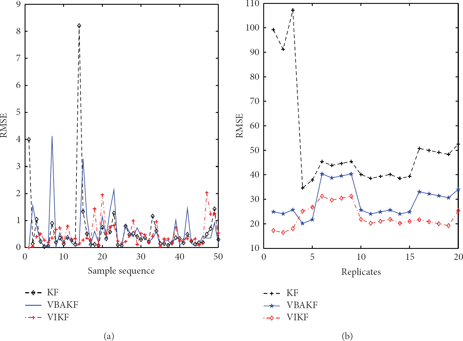
The RMSE performances of VIKF, VBAKF, and KF are shown in Figure 1, Figure 2 (for Student's t-distribution), and Figure 3 (for Gaussian distribution). The results shown in Figure 1(a) show the RMSE of each state, which are obtained by averaging the results of the 20 replicates. Figure 1(b) shows the accumulated RMSE of all steps for each replicate. A typical simulation result is also shown in Figure 2. In these figures, we restrict the display range of the Y-axis to show the results clearly, so some points with high RMSE cannot be seen. We can see that the performance of VIKF is clearly higher than that of VBAKF and KF in the case of noise with Student's t-distribution. KF and VBAKF all have a higher probability of occurring extreme RMSE in certain circumstances, while the VIKF algorithm has a relatively lower probability. The reason that VIKF can decrease the probability of occurring large RMSE is that VIKF can perform sufficient iterations.

Figure 1

Performances of VIKF, VBAKF, and KF for the case of Student's t-distribution. (a) The RMSE of each state obtained by averaging the results of 20 replicates. (b) The accumulated RMSE of all 30 steps for each replicate.

Figure 2

A typical simulation result with Student's t-distribution in high-dimensional linear state space.

Figure 3

Performances of VIKF, VBAKF, and KF for the case of Gaussian distribution. (a) The RMSE of each state obtained by averaging the results of 20 replicates. (b) The accumulated RMSE of all 30 steps for each replicate.

In the case of Gaussian noise, the performances of these three algorithms are close, as shown in Figure 3.

4.2. Tracking in WSN

The state space for the tracking problem in WSN was fixed as in Section 4, included two-dimensional coordinates and two-dimensional velocities. As the simulations in Section 4.1, we considered two kinds of noise: Gaussian distribution and Student's t-distribution. We assume that there are 15 sensor nodes and 50 sampling points. Noise was set as that in Section 4.1.

As Figures 1 and 3, Figure 4 shows the RMSE performances with Student's t-distribution noise, where Figure 4(a) shows the RMSE of each state obtained by averaging the results of 20 replicates and Figure 4(b) shows the accumulated RMSE of all steps for each replicate. Figure 5 shows the corresponding results with Gaussian noise. Figure 6 shows the tracking performance using the three algorithms with noise of Student's t-distribution.

Figure 4

Performances of VIKF, VBAKF, and KF for the case of Student's t-distribution. (a) The RMSE of each state obtained by averaging the results of 20 replicates. (b) The accumulated RMSE of all 50 steps for each replicate.

Figure 5

Performances of VIKF, VBAKF, and KF for the case of Gaussian distribution. (a) The RMSE of each state obtained by averaging the results of 20 replicates. (b) The accumulated RMSE of all 50 steps for the 20 replicates.

Figure 6

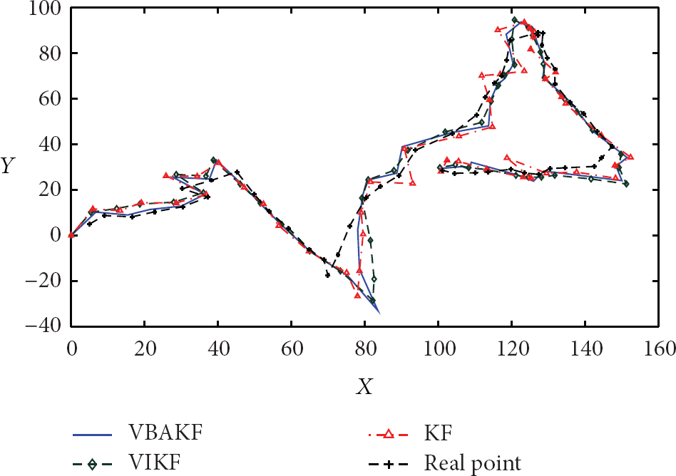
Tracking performances of VIKF, VBAKF, and KF with Student's t-distribution noise.

With the noise of Student's t-distribution, the performance of VIKF in tracking is higher than that of VBAKF and KF. VIKF's probability of high RMSE is also lower than KF and VBAKF. In Gaussian cases, it seems that the performance of KF is better than that of VBIKF and VIKF.

5. Conclusions

This paper used variational approximation method to solve the problems arisen from high-dimensional discrete state space and the tracking problems in WSN with linear state model. We proposed a modified variational filtering algorithm, in which an iterative process was formed to get the optimization solutions.

The performance of variational methods is slightly lower than that of KF in a Gaussian environment. But in non-Gaussian and time-varying noise environment, the average performances of VIKF and VBAKF are better than that of KF. Since VIKF can carry out more sufficient iterations than the VBAKF in the update step, the performance of VIKF is better than that of VBAKF. VIKF algorithm also has a lower probability of high RMSE than KF and VBAKF in non-Gaussian environments.