Anchor-Node-Based Distributed Localization with Error Correction in Wireless Sensor Networks

Abstract

This paper proposes a scheme to enhance localization in terms of accuracy and transmission overhead in wireless sensor networks. This scheme starts from a basic anchor-node-based distributed localization (ADL) using grid scan with the information of anchor nodes within two-hop distance. Even though the localization accuracy of ADL is higher than that of previous schemes (e.g., DRLS), estimation error can be propagated when the ratio of anchor nodes is low. Thus, after each normal node estimates the initial position with ADL, it checks whether the position needs to be corrected because of the insufficient anchors within two-hop distance, that is, the node is in sparse anchor area. If correction needs, the initial position is repositioned using hop progress by the information of anchor nodes located several hops away so that error propagation is reduced (REP); the hop progress is an estimated hop distance using probability based on the density of sensor nodes. Results via in-depth simulation show that ADL has about 12% higher localization accuracy and about 10% lower message transmission cost than DRLS. In addition, the localization accuracy of ADL with REP is about 30% higher than that of DRLS, even though message transmission cost is increased.

1. Introduction

Many applications of wireless sensor networks such as object tracking, environment and habitat monitoring, intrusion detection, and geographic routing rely on the location information of sensor nodes [1]. To provide accurate position information of sensor nodes, each sensor node can be equipped with GPS [2]. In many applications, however, it is not possible that all sensor nodes are equipped with GPS economically and technically. For examples, GPS signal hardly reaches to all nodes when wireless sensor networks are deployed in underground structure or underwater environments, where a sensor node must estimate its position from various information of other nodes that are possibly equipped with GPS or estimate their positions from others as well. A localization refers to a process for determining the position of users or wireless devices without using positioning hardware device as GPS [3, 4].

Localization schemes are categorized into two classes: range-based positioning scheme and range-free positioning scheme. A range-based positioning scheme measures the distance or the angle between sensor nodes and estimate positions using triangulation, trilateration, and multilateration algorithms. Typical range-based positioning schemes include Time of Arrival (ToA) [5], Time Difference of Arrival (TDoA) [6], Angle of Arrival (AoA) [7], Received Signal Strength Indicator (RSSI) [8], and RSS-based localization using direction calibration [9]. The range-based positioning schemes require additional devices to measure the distance or the angle between sensor nodes. Some range-based positioning schemes are sensitive to temporary interference of signal such as noise and fading. They are unsuited to massive wireless sensor networks. A range-free scheme estimates positions using connectivity information between sensor nodes [10–20]. Among the range-free positioning schemes are Centroid [10], Convex Position Estimation (CPE) [11], and Distance Vector-Hop (DV-Hop) [12] methods. The range-free positioning schemes, however, suffer from high message transmission cost to gather the connectivity information and high computational cost to estimate positions of sensor nodes. In addition, they have shown high position estimation error compared to other methods.

Distributed Range-free Localization Scheme (DRLS) [21] improved localization accuracy of normal nodes by utilizing anchor nodes within two-hop distance. The scheme used grid scanning algorithm to estimate the initial position of a normal node and tried to improve the estimation accuracy by vector-based refinement. The vector-based refinement, however, could inaccurately decide the position of normal nodes depending on the relative position of anchor nodes and needs square-root calculations requiring high computation power. In addition, a normal node can infer an incorrect localization when it estimates its position from other normal nodes due to the lack of neighbor anchor nodes. The incorrect localization of a normal node deteriorates the localization of another normal node so that the error is propagated over the networks.

This paper proposes an Anchor-based Distributed Localization (ADL) scheme and its Reducing Error Propagation (REP) scheme. The ADL devises a grid scanning algorithm of two-hop anchor nodes instead of the vector-based refinement of DRLS, which reduces the computational cost occurred by the refinement of DRLS and improves the accuracy of the localization. The ADL with REP enhances the initial estimation of a normal node that does not have anchor nodes within two-hop and reduces the impact of the error propagation frequently occurred with a sparse anchor nodes deployment. Our contributions in this paper are as follows.

• (i)

We designed a basic ADL to improve the accuracy of the localization and reduce the computational cost, and proposed an REP scheme based on ADL to decrease the propagation error in the sparse anchor nodes deployment, as previous work [22, 23]. In this paper, we organize the ADL with REP and then develop the various simulation environments to evaluate our scheme from the several points of view.

(ii)

The results via in-depth simulation show that the basic ADL has about 12% higher localization accuracy and about 10% lower message transmission cost than DRLS. In addition, the localization accuracy of ADL with REP is about 30% higher than that of DRLS, even though message transmission cost is increased.

The remainder of the paper is organized as follows: Section 2 presents preliminary study and previous work. Section 3 details our proposed scheme. Section 4 discusses simulation results. Finally, Section 5 concludes the paper.

2. Preliminaries and Related Work

2.1. Assumptions and Definition

The purpose of the proposed scheme is to provide more accurate localization by applying a range-free localization scheme. In the range-free localization scheme, we assume that a sensor network consists of normal nodes and anchor nodes, where the normal nodes do not know their position but the anchor nodes are able to acquire their positions via external positioning device such as GPS. All sensor nodes including the normal node and the anchor node are randomly deployed in a sensor field, and they do not move after the initial deployment. In addition, each sensor node has a unique ID and the same data transmission radius [21].

In the proposed scheme, each normal node estimates its position by obtaining position information from anchor nodes within two-hop distance. An one-hop anchor node is an anchor node located within the data transmission radius r of a normal node. A two-hop anchor node is reachable by a normal node with a two-hop path alone. For an anchor node to be a two-hop anchor, the anchor is located within twice transmission range ( $2r$ ) of the normal node, but out of a transmission range. Figure 1 shows an example of one-hop and two-hop anchor nodes. Normal node $N_1$ considers anchor nodes $A_1$ and $A_2$ are one-hop anchor nodes because they are located within transmission radius of $N_1$ . Anchor node $A_3$ is a two-hop anchor node of $N_1$ that indirectly obtains the position information of $A_3$ via a normal node $N_2$ .

Figure 1

An example of one- and two-hop anchor nodes ( $A_1$ and $A_2$ are one-hop anchor nodes of $N_1$ and $N_2$ , and $A_3$ is a two-hop anchor node of $N_1$ .).

2.2. Related Work

In the range-free localization scheme, a normal node estimates its position using connectivity information between itself and its neighbor nodes. Thus, the scheme requires data transmission instead of additional devices to measure distances or angles between sensor nodes. In Centroid [10], each normal node estimates its position by calculating the average position of the neighbor anchor nodes, after gathering the position information of neighbor anchor nodes. This localization method is very simple but its accuracy becomes very low when there are a few sensor nodes in the field. In addition, its localization accuracy is highly depending on the deploying pattern of anchor nodes.

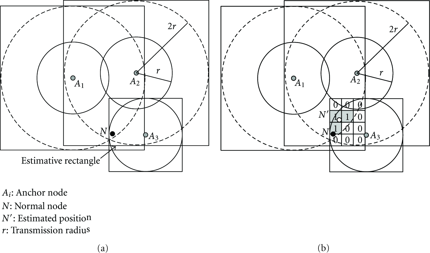
Convex position estimation (CPE) [11] proposed to relieve the wrong localization issue of the Centroid based on the position of anchor nodes. CPE also uses the connectivity information between sensor nodes, where each normal node assumes an imaginary rectangle, or an estimative rectangle (ER) that is tangent to an overlapped region of transmission radiuses of neighbor anchor nodes. The normal node should be on ER and the center of the rectangle is approximated as the estimated position of the normal node.

Distributed Range-free Localization Scheme (DRLS) [21] extends to use anchor nodes within two-hop distance. The scheme consists of two phases as initial placement (i.e., grid scan) and refinement. In the initial placement phase, the transmission range of each anchor node is virtually considered as a square instead of a circle and a normal node N assumes an ER as a region overlapped by the squares of anchor nodes within one-hop distance from the normal node. The ER calculated by this method covers a larger area than the one of CPE does. To compensate this looseness, the scheme applies a grid scanning so that the ER is divided to small grid-shaped cells. The number of times each cell overlaps with the transmission range of anchor nodes is calculated. The gray cells in Figure 2(a) have the highest value that is the number of nesting and the normal node N should be on these cells. The average position of gray cells, $N^{\prime }$ , is estimated as the initial position. If a normal node is in two-hop path of an anchor node, the second phase allows refining its position. Figure 2(b) shows the refinement phase of DRLS. Because the normal node N cannot be in the transmission radius of anchor node $A_3$ that is within two-hop distance from N, the initial estimated position $N^{\prime }$ is adjusted using a virtual force ( $\text{V}{\text{F}}_{{\text{A}}_3}$ ) that is made by the effect of $A_3$ to the region formed by $A_1$ and $A_2$ . The direction of $\text{V}{\text{F}}_{{\text{A}}_3}$ is from $A_3$ to $N^{\prime }$ , and the length of $\text{V}{\text{F}}_{{\text{A}}_3}$ is $|\stackrel{⃗}{{VF}_{{\text{A}}_3}}|=\overline{ab}·\overline{N^{1}c}/\overline{ac}$

Figure 2

An example of the position estimation by DRLS: (a) initial position estimation by grid-scan; (b) refinement of initial position.

However, DRLS has some problems. First of all, two-hop flooding of DRLS is based on anchor nodes. Each anchor node exchanges its position information with anchor nodes that are located within two-hop distance and provides all of information to its neighbor normal nodes. Even though normal nodes obtain some position information during the information exchange between anchor nodes, the normal nodes do not use the information. Secondly, localization accuracy can be worse depending on the deployment pattern of sensor nodes in the refinement phase as illustrated in Figure 3. $N^{\prime }$ is obtained as the estimated position of a normal node N by an one-hop anchor node $A_3$ . Two-hop anchor nodes $A_1$ and $A_2$ decide the VF as the sum of the $\text{V}{\text{F}}_{{\text{A}}_1}$ and $\text{V}{\text{F}}_{{\text{A}}_2}$ , so that $N^{\prime \prime }$ can be forced to be at the position where the normal node cannot be located. At the last but the most importantly, normal nodes with no neighbor anchor nodes estimate their positions with the position information of neighbor normal nodes that already have some localization errors. The error propagation causes a serious problem in many situations. Figure 4 shows an example of frequently occurring error propagation. When two anchor nodes are located together, such as $A_1$ and $A_2$ , the estimated position, such as $N_1^{\prime }$ , $N_2^{\prime }$ , and $N_3^{\prime }$ , is on the line connecting two anchor nodes, even though the real positions of normal nodes are $N_1$ , $N_2$ , and $N_3$ . The error propagation is amplified by the distance from anchor nodes. In this paper, we propose a novel scheme substitutes the vector-based refinement and reduces error propagation to resolve the problems discussed above.

Figure 3

An example that localization error increases in the refinement of DRLS.

Figure 4

An example of error propagation in DRLS when two anchor nodes are distributed together.

3. Anchor-Node-Based Distributed Localization with Error Correction

This section presents the basic ADL and advances the ADL with error correction to reduce the error propagation in sparse anchor node environments. Figure 5 outlines our proposed scheme, the ADL with ERP. Each normal node obtains an initial estimated position after performing ADL, and then it check whether the position needs to be corrected because of the insufficient anchors within two-hop, that is, the node is in sparse anchor area. If yes, each node estimates the final position by hop progress, otherwise, the initial position becomes a final value.

Figure 5

Outline of proposed localization scheme.

3.1. Basic ADL

The Basic ADL consists of three steps: anchor node selection, ER construction, and distributed grid scan. We introduce the steps and the limitation of ADL in sparse anchor node environments.

3.1.1. Anchor Node Selection

In the anchor node selection step, two-hop flooding is used for normal nodes to obtain the information of anchor nodes within two-hop distance. Two-hop flooding is started from each anchor node, and each anchor node broadcasts its ID and position information to its neighbor sensor nodes. All normal nodes that receive the information broadcasted decide the anchor nodes of the information obtained as their one-hop anchor nodes. Then, the normal nodes that have the information of one-hop anchor nodes broadcast the information of their one-hop anchor nodes to its neighbor normal nodes. The normal nodes that receive the information of the one-hop anchor nodes from their neighbor sensor nodes consider the anchor nodes of the information obtained as two-hop anchor nodes.

3.1.2. ER Construction

A normal node can be located in a rectangle with thick lines of Figure 6(a). However, it is very difficult to calculate this region, since the region is presented by the subsumption relationship between circles. Therefore, an approximate region termed ER is determined by rectangles that are tangential to the transmission radius of each anchor node, to find this region with lower computational cost. Rectangles, that are tangential to the circles whose centers are the positions of one-hop anchor nodes and radiuses are the transmission radius of sensor nodes, are formed to create ER. In addition, rectangles that are tangential to the circles whose centers are the positions of two-hop anchor nodes and radiuses are the two times of transmission radius, are made. Subsequently, the overlapped region of all rectangles is selected as ER. Figure 6(a) shows an example to form an ER as the overlapped region of three rectangles.

Figure 6

An example of ER construction and grid scan: (a) ER construction; (b) grid Scan.

3.1.3. Distributed Grid Scan

The ER calculated by a normal node includes a region that is larger than the region in which the normal node can actually exist. Accordingly, the localization accuracy can be enhanced by excluding the region where a normal node cannot actually exist from the ER using the grid scan algorithm. After dividing the ER into a set of grid cells, the normal node scans each cell to decide if the cell region should be excluded as shown in Figure 6(b). When the data transmission radius is r, the length of the edge on each cell is $0.1r$ by considering the scanning computational cost and localization accuracy. Each cell has a binary value as a representative value initialed by 1. The binary value 1 denotes that the normal node can exist in the cell. While scanning the cells, the normal node excludes cells in which the normal node cannot be located (i.e., setting 0 to the excluded cells). The center of gravity on each cell is deemed to be the representative position of the cell. Finally, normal node N obtains final estimated position $N^{\prime }$ by computing the average of the representative coordinate values in each shaded cell with 1 as shown in Figure 6(b).

In this paper, the scanning method is applied differently to one- and two-hop anchor nodes. If the normal node has two-hop anchor nodes, the values of cells, that are located within the data transmission radius r of each two-hop anchor node or outside a circle of radius $2r$ of each two-hop anchor node, are changed to 0 that means the normal node cannot be located in the cell. If the normal node has one-hop anchor nodes, the values of cells that are located outside of data transmission radius r are changed to 0. After scanning all of cells, the average coordinate of cells whose values are 1 is calculated as the estimated position of the normal node. Figure 6 shows an example of grid scanning. The ER formed in Figure 6 should be divided by many cells; however, we divide ER by 12 cells to understand it easily. The result of the grid scanning shows that the estimated position of a normal node N is $N^{\prime }$ , and $N^{\prime }$ is used as the initial position of the normal node when correcting the position in Section 3.2.

Since sensor nodes are deployed in the sensor field randomly, there can be normal nodes without any information of anchor nodes. Such normal nodes wait until the neighbor normal nodes estimate and broadcast their position. Then, they estimate their position by the information from neighbor normal nodes. For the estimation by neighbor normal nodes, all normal nodes that obtain their position, broadcast their position information and their one-hop anchor nodes. The normal nodes, that do not have any position information of an anchor node, receive the information of neighbor normal nodes and mark one-hop anchor nodes of the neighbor normal nodes as two-hop anchor nodes. They then perform the same ER construction and distributed grid scan as just explained steps.

3.2. Reducing Error Propagation (REP)

The REP handles only the error propagation by neighbor positions with low precision (e.g., one case that two anchor nodes are located together, thus error propagation would be enlarged as shown Figure 4, or the other case by insufficient anchor nodes within two-hop). Through hop progress calculation and repositioning, REP corrects the position information of normal nodes by rotating the estimated positions centering on anchor nodes. Lastly in this subsection, we explain about decision method for whether to apply REP.

3.2.1. Hop Progress Calculation

To reduce error propagation, other information is necessary for adjusting position information. REP uses the information of anchor nodes that is multihop away from normal nodes. Normal nodes can obtain the information of anchor nodes multihop away when other normal nodes finishing to estimate the initial position and broadcasting their position to their neighbor normal nodes. When sending information of themselves to their neighbor sensor nodes after completing to estimate their initial position, normal nodes that have neighbor anchor nodes send not only their estimated position information but also the position information of an one-hop anchor node and the distance between the normal node and the one-hop anchor node. The anchor node information obtained first is used as the center of the rotation. Moreover, the center of the rotation of each normal node that does not have any neighbor anchor nodes is fixed for the center of the rotation of the neighbor normal node. The distance between the normal node and the center of the rotation is determined by hop progress (i.e., an estimated hop distance using probability based on the density of sensor nodes) [24]. The density of normal nodes means the average number of sensor nodes in the transmission radius of a sensor node. Hop progress can be derived from (1) [24, 25]. In (1), $E(R)$ is the estimated hop progress, $E_C$ is the sensor node density, and $r_0$ is the transmission radius. Hop progress is calculated by only the sensor node density and the data transmission radius:

$E\left(R\right)=\frac{2\left(E_C+1\right)\sin \theta }{\pi {r_0}^2}{{\displaystyle \int }}_0^{r_0}{l}^2{e}^{-\left(\right(E_C+1)/\pi )\theta (1-(l^2/{r_0}^2\left)\right)}dl.$

(1)

Each normal node estimates the distance between itself and the center of the rotation using hop progress. Then, the normal node broadcasts the position information of the center of the rotation and hop progress to the position for neighbor normal nodes that do not have any information of anchor nodes. This broadcast can be efficient by adding the information of the center of the rotation to the broadcast packet after the grid-scan phase. Through this procedure, all normal nodes have position information of 1~3 anchor nodes and hop progress to the anchor nodes as well as their initial position.

3.2.2. Repositioning

Each normal node that has the position information of three anchor nodes and hop progress to the anchor nodes corrects its initial position using its information obtained. Each normal node calculates two cross-points of two circles whose center point is the center of the rotation and radius is the hop progresses of two anchor nodes. These two cross-points are regarded as the position in which the normal node can be located. However, since the hop progresses are based on the probability, the accuracy of these two cross-points are low. Thus, these two points are used not to correct the initial position directly, but to decide the direction of the rotation. The direction of the rotation is decided as a cross-point of two circles that is nearer by the third anchor node that is not used to make two circles. The reason of the selection between two cross-points is that the cross-point far from the third anchor node cannot receive the information of the third anchor node.

To correct the initial position of a normal node by rotation, the angle of the rotation is necessary. As knowing the initial position and the center and the direction of the rotation, the normal node can obtain the angle of the rotation. Figure 7 shows an example of the center and the angle of the rotation, and the angle of the rotation can be obtained by (2):

$\cos \theta =\frac{d{\left(A_1,D\right)}^2+d{\left(A_1,{N_1}^{\prime }\right)}^2-d{\left({N_1}^{\prime },D\right)}^2}{2\cdot d\left(A_1,D\right)\cdot d\left(A_1,{N_1}^{\prime }\right)}.$

(2)

Figure 7

Deciding the direction of the rotation with the information of three anchor nodes.

In (2), $d(a,b)$ is the Euclidean distance between the point a and b. The value of $\sin \hspace{0.17em}\theta$ can be a positive or negative value, so the normal node should decide the presence of the negative sign. When the coordinate of $A_1$ is ( $x_{A_1}$ , $y_{A_1}$ ), the coordinate of ${N_1}^{\prime }$ is ( $x_{{N_1}^{\prime }}$ , $y_{{N_1}^{\prime }}$ ), and the coordinate of the rotation direction D is ( $x_D$ , $y_D$ ), $\sin \hspace{0.17em}\theta$ is calculated in (3) by the relation between the line $A_1{N_1}^{\prime }$ and the position D:

$\sin \theta =\{\begin{array}{c}\begin{array}{cc}\sqrt{1-{\left(\cos \theta \right)}^2},& \text{if}\hspace{0.17em}\hspace{0.17em}\left({\phantom{\sqrt{1-{\left(\cos \theta \right)}^2}}x}_{{N_1}^{\prime }}-x_{A_1}\ge 0,\hspace{0.17em}\hspace{0.17em}\left(x_{{N_1}^{\prime }}-x_{A_1}\right)\left(y_D-y_{A_1}\right)\ge \left(y_{{N_1}^{\prime }}-y_{A_1}\right)\left(x_D-x_{A_1}\right)\right)\\ & \text{or}\hspace{0.17em}\hspace{0.17em}\left(x_{{N_1}^{\prime }}-x_{A_1}<0,\hspace{0.17em}\hspace{0.17em}\left(x_{{N_1}^{\prime }}-x_{A_1}\right)\left(y_D-y_{A_1}\right)<\left(y_{{N_1}^{\prime }}-y_{A_1}\right)\left(x_D-x_{A_1}\right)\right)\\ -\sqrt{1-{\left(\cos \theta \right)}^2},& \text{otherwise}.\end{array}\hfill \end{array}$

(3)

Then, the coordinate of ${N_1}^{\prime \prime }$ , ( $x_{{N_1}^{\prime \prime }}$ , $y_{{N_1}^{\prime \prime }}$ ) that is the rotatory translation of ${N_1}^{\prime }$ with the angle of rotation θ is obtained in (4):

$\left(\begin{array}{c}{x}_{{N_1}^{\prime \prime }}\\ y_{{N_1}^{\prime \prime }}\end{array}\right)=\left(\begin{array}{cc}\cos \theta & -\sin \theta \\ \sin \theta & \cos \theta \end{array}\right)\left(\begin{array}{c}{x}_{{N_1}^{\prime }}-x_{A_1}\\ y_{{N_1}^{\prime }}-y_{A_1}\end{array}\right)+\left(\begin{array}{c}{x}_{A_1}\\ y_{A_1}\end{array}\right).$

(4)

In Figure 8, ${N_1}^{\prime \prime }$ that is the corrected position by rotatory translation is closer to $N_1$ , that is the real position of the normal node, than the initial position ${N_1}^{\prime }$ . The normal nodes that complete REP broadcast their estimated position information to apply REP to the normal nodes that have one or two anchor node information.

Figure 8

Amending the position with the initial estimated position and the direction.

3.2.3. Decision for Applying REP

REP does not always reduce the estimation error. Even though REP is applied to amend the initial estimated positions of normal nodes, the error of the localization can be increased when the initial estimated positions are relatively correct. Therefore, whether to apply REP is decided for more accurate localization. Each normal node compares the variations of estimated positions before and after applying REP. The variation of the estimated position means the degree of error. The bigger the region that a normal node can be located in is, the bigger the variation is. When the variation of estimate position after applying REP is smaller than that before applying REP, REP is applied to the initial estimated position. On the contrary, the initial estimated position is decided as the final estimated position when the variation of estimate position after applying REP is bigger than that before applying REP. Generally, normal nodes that are close to anchor nodes have low variance for the estimated position, since the degree of error propagation is relatively small when normal nodes that are close to anchor nodes estimate their initial position.

4. Performance Evaluation

This section handles the performance results of ADL and ADL with REP. To show the degree of performance improvement, ADL and ADL with REP are compared to DRLS, a previous range-free localization scheme. The earlier part of this section presents the simulation environment, and the metrics and parameters of performance evaluation. The later part of this section presents the localization accuracy and message transmission cost of DRLS, ADL, and ADL with REP.

4.1. Methodology

The simulator in this section is realized using JAVA. Data transmission radiuses of all sensor nodes are same as r in the simulation of ADL and ADL with REP. The unit disk model [26] is used to transmit data. That is, a sensor node transmits data successfully to its neighbor sensor nodes that are located within r. The same sensor nodes are deployed randomly on the sensor field whose size is $10r\times 10r$ . A few anchor nodes that equip GPS know their real position. All sensor nodes are the same, except for the existence of GPS. The collision that occurs during message transmission for the position estimation is not considered. The cell size of the grid scan phase in ADL is fixed to $0.1r\times 0.1r$ . All simulation results are based on 100 repetitions.

The metrics for the performance evaluation are localization accuracy, mean squared error (MSE), and message transmission cost.

• (1)

Localization accuracy. Localization accuracy is defined as the average of the Euclidean distance between the real positions and the estimated positions of all normal nodes. The data transmission radius r is the basic unit of localization accuracy. Localization accuracy denotes how accurately normal nodes estimate their positions.

(2)

Mean squared error (MSE). MSE for the estimated position of normal nodes denotes the degree of variance of the estimated position of normal nodes.

(3)

Message transmission cost. Message transmission cost is the number of messages used for normal nodes to obtain the information of anchor nodes.

The parameters for the simulation are the density of sensor nodes and the ratio of anchor nodes. The density of the sensor nodes is diversified by the change of the number of sensor nodes, and the number of anchor nodes is changed for the density of sensor nodes to be varied over the entire sensor field. Since the ratio of the anchor nodes is controlled by the fixed number of sensor nodes deployed in the sensor field, the number of normal nodes is decreased if the number of anchor nodes is increased.

4.2. Average Error and Mean Squared Error with Different Anchor Ratio

This section analyzes the localization accuracy and MSE of ADL and ADL with REP versus the ratio of anchor nodes. The data transmission radius of each sensor node is r. The simulation is performed against various numbers of sensor nodes, such as 200, 400, 600, and 800 in the sensor field whose size is $10r\times 10r$ , in addition, the ratio of anchor nodes is changed from 5 to 30% for each number of sensor nodes.

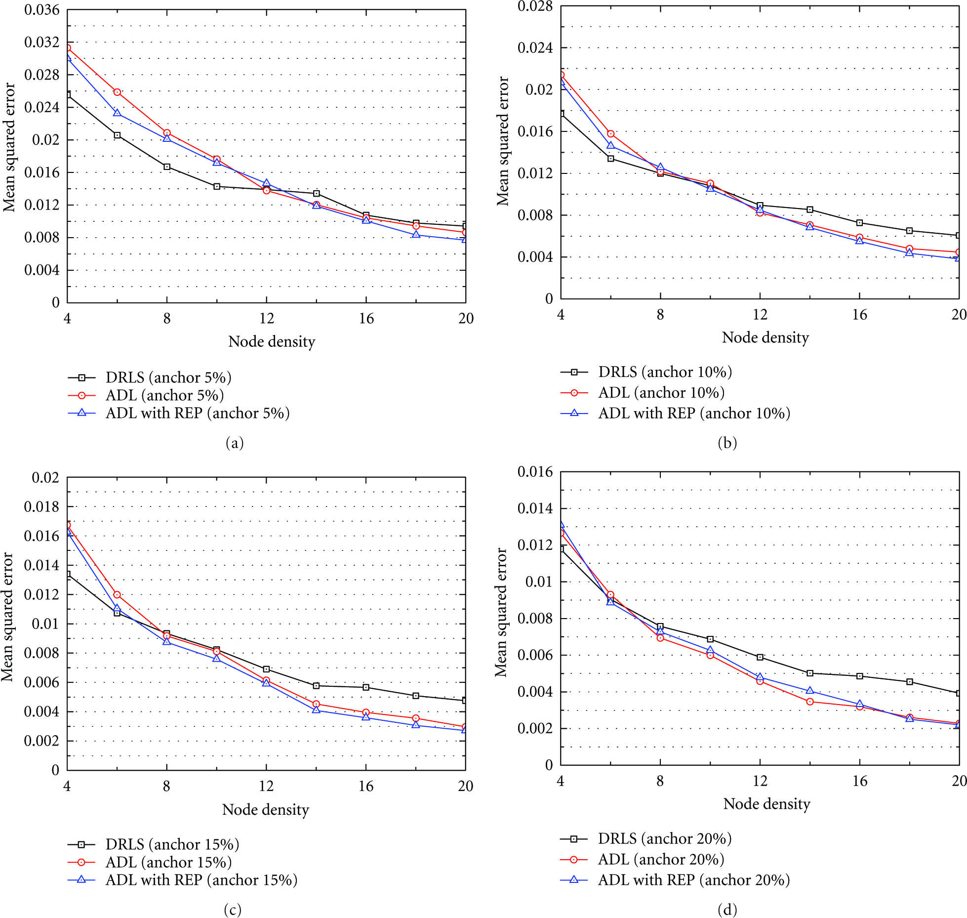
Figure 9 shows the mean error of the estimated position of DRLS, ADL, and ADL with REP in accordance with the variety of the ratio of anchor nodes. Localization accuracy of ADL with REP is the highest, and that of DRLS is the least, since ADL increases the localization accuracy by estimating the position of normal nodes without the vector-based refinement of DRLS. ADL with REP amends the initial estimated position of normal nodes in ADL by applying REP. The lower the ratio of anchor nodes is, the fewer the amount of the position information of anchor nodes is; therefore, localization accuracy is decreased. When the number of sensor nodes is low, localization accuracy is relatively low due to the hole problem. Moreover, when the number of the sensor nodes is high, localization accuracy is increased due to the increase in the information that a normal node can obtain. When there are 800 sensor nodes, the difference of localization accuracy between ADL and ADL with REP is little due to the fact that the initial estimated positions are already sufficiently accurate, and the estimation error can be increased by REP. The simulation results show that ADL with REP has a maximum of 18% higher accuracy compared to ADL and a maximum of 30% higher accuracy compared to DRLS, when there are 400 sensor nodes.

Figure 9

Mean error versus anchor ratio: (a) the number of sensors is 200; (b) 400; (c) 600; (d) 800.

Figure 10 shows MSE of DRLS, ADL, and ADL with REP versus the ratio of anchor nodes. Except for the cases with 200 and 800 sensor nodes, ADL with REP has the lowest MSE, and DRLS has the highest MSE since ADL with REP has the least variance of the estimated position by reducing error propagation. For 200 sensor nodes, MSE of DRLS is the lowest when the ratio of the anchor nodes is low, since the number of normal and anchor nodes is small and thus each normal node cannot receive the sufficient position information. When there are 800 sensor nodes, the MSE of ADL of REP is high, since the normal nodes, whose positions are already accurate, amend their positions by REP, so that the position estimation error is increased. The simulation results show that ADL with REP has a maximum of 7% lower MSE compared to ADL and a maximum of 22% lower MSE compared to DRLS when there are 400 sensor nodes.

Figure 10

MSE versus anchor ratio: (a) the number of sensors is 200; (b) 400; (c) 600; (d) 800.

4.3. Average Error and Mean Squared Error with Different Sensor Node Density

This section analyzes the localization accuracy and MSE with various densities of sensor nodes. The density of sensor nodes is defined as the average number of sensor nodes within the data transmission radius of a sensor node. When the data transmission radius is r, if 200 sensor nodes are deployed in the sensor field whose size is $10r\times 10r$ , the number of sensor nodes in the data transmission radius is 6.28. The simulation is performed with anchor ratios of 5, 10, 15, and 20%, and the density of sensor nodes is changed from 4 to 20 in each density of anchor nodes.

Figure 11 shows the localization accuracy versus the density of sensor nodes. Mean error of ADL with REP is the smallest and that of DRLS is the largest, since ADL increases localization accuracy by estimating the position of normal nodes without the vector-based refinement of DRLS. ADL with REP amends the initial estimated position of normal nodes in ADL by applying REP. When the ratio of anchor nodes is 20% and the density of sensor nodes is 4, mean error of ADL is lower than that of ADL with REP since the number of both normal nodes and anchor nodes is small and thus accurate position estimation is impossible. The simulation results show that ADL with REP has a maximum of 13% higher accuracy compared to ADL and a maximum of 25% higher accuracy compared to DRLS when the density of anchor nodes is 10%.

Figure 11

Mean error versus node density: (a) anchor ratio is 5%; (b) 10%; (c) 15%; (d) 20%.

Figure 12 shows the MSE versus the various densities of sensor nodes. Due to the fact that more accurate position estimation is possible with many sensor nodes, the higher the density of sensor nodes is, the lower the MSE is. When the density of sensor nodes is low, MSE of DRLS is the lowest since normal nodes cannot receive sufficient position information from the small number of normal and anchor nodes. When the ratio of anchor nodes is 20%, MSE of ADL is lower than that of ADL with REP, since normal nodes whose initial estimated positions are sufficiently accurate from many anchor nodes amend their positions by REP so that MSE is increased. When the ratio of anchor nodes is 10%, the simulation results show that ADL with REP has a maximum of 8% lower MSE compared to ADL, and a maximum of 28% lower MSE compared to DRLS with an environment whose node density exceeds 12.

Figure 12

MSE versus node density: (a) anchor ratio is 5%; (b) 10%; (c) 15%; (d) 20%.

4.4. Message Transmission Cost

This section analyzes the message transmission cost for position estimation by ADL and ADL with REP. This cost is defined as the number of messages exchanged. The simulation environment is changed with the ratio of anchor nodes from 5 to 30% and the density of sensor nodes from 4 to 20.

Figure 13 shows the message transmission cost against various ratios of anchor nodes. Due to the fact that two-hop flooding is performed based on the anchor nodes in DRLS and based on normal nodes in ADL, the message transmission cost of ADL is the lowest. That is, each anchor node in DRLS exchanges its position information with anchor nodes that are located within two-hop distance, and provides all of information to its neighbor normal nodes. Even though normal nodes in DRLS obtain some position information during the information exchange between anchor nodes, anchor nodes after finishing the two-hop flooding transmit the information to normal nodes. Due to such unnecessary transmissions of DRLS, ADL outperforms DRLS a little from the viewpoint of transmission cost. The higher data transmission cost of ADL with REP is due to each normal node broadcasting the information of their center of the rotation additionally after applying REP. Generally, DRLS transmits more messages as many as the number of anchor nodes than ADL, and ADL with REP transmits more messages as many as the number of normal nodes than ADL. The simulation results show that the message transmission cost of ADL with REP is a maximum of 45% higher than ADL when the ratio of anchor nodes is low, and a maximum of 35% higher than DRLS when the number of sensor nodes is 400 and the ratio of anchor node is 10%.

Figure 13

Number of messages versus anchor ratio: (a) the number of sensors is 200; (b) 400; (c) 600; (d) 800.

Figure 14 shows the message transmission cost against various densities of sensor nodes. Like Figure 13, the message transmission cost of ADL is the lowest and that of ADL with REP is the highest since two-hop flooding of ADL is more efficient than that of DRLS. ADL with REP makes normal nodes to amend their initial estimated positions by additional message transmissions. When the ratio of anchor nodes is low such as 5%, in ADL with REP, normal nodes transmit their center of the rotation to their neighbor normal nodes additionally after applying REP, so there is a big gap between transmission costs of ADL and ADL with REP. The simulation results show that the message transmission cost of ADL with REP is a maximum of 45% higher than ADL and that of ADL is a maximum of 7% lower than DRLS when the ratio of anchor nodes is 10% and the density of sensor nodes is 10.

Figure 14

Number of messages versus node density: (a) anchor ratio is 5%; (b) 10%; (c) 15%; (d) 20%.

5. Conclusions

The paper has proposed ADL that is a distributed localization scheme to increase the position accuracy and reduce the message transmission cost, and ADL with REP that is a scheme to reduce the error propagation. In ADL, each normal node assumes an ER using anchor nodes within its transmission radius that is obtained by two-hop flooding, and initial position is estimated by grid scanning in the ER. However, since the initial estimated positions are affected by the error propagation in the environment with the small number of anchor nodes, initial estimated positions should be amended. The ADL with REP makes normal nodes to estimate their position more accurately by rotating the initial estimated positions whose centers are anchor nodes.

The simulation results with the various ratios of anchor nodes and the various densities of sensor nodes showed that localization accuracy of ADL is 12% higher and the data transmission cost is 10% lower than DRLS. In addition, localization accuracy of ADL with REP is 30% higher, but the data transmission cost is 35% higher than DRLS. Due to the fact that the data transmission cost of ADL with REP is high, we should decide a scheme among ADL and ADL with REP according to the application. We will enhance the proposed localization in order that the case whereby the amended position is more inaccurate than the initial estimated position by applying REP is avoided by the statistical analysis.