Error-Tolerant and Energy-Efficient Coverage Control Based on Biological Attractor Selection Model in Wireless Sensor Networks

Abstract

A coverage problem is one of the important issues to prolong the lifetime of a wireless sensor network while guaranteeing that the target region is monitored by a sufficient number of active nodes. Most of existing protocols use geometric algorithm for each node to estimate the degree of coverage and determine whether to monitor around or sleep. These algorithms require accurate information about the location, sensing area, and sensing state of neighbor nodes. Therefore, they suffer from localization error leading to degradation of coverage and redundancy of active nodes. In addition, they introduce communication overhead leading to energy depletion. In this paper, we propose a novel coverage control mechanism, where each node relies on neither accurate location information nor communication with neighbor nodes. To enable autonomous decision on nodes, we adopt the nonlinear mathematical model of adaptive behavior of biological systems to dynamically changing environment. Through simulation, we show that the proposal outperforms the existing protocol in terms of the degree of coverage per node and the overhead under the influence of localization error.

1. Introduction

A wireless sensor network [1] has been attracting many researchers over the past ten years for a variety of its applications [2]. Among them, surveillance, monitoring, and observation of items, objects, and regions are most promising and useful. These applications require that a sufficient number of sensor nodes monitor the target region. Due to the uncertainty and instability of location and sensing area, it is difficult to deploy and manage sensor nodes in an optimal manner, that is, placing a minimum number of sensor nodes at the optimal positions. Therefore, a redundant number of sensor nodes are generally deployed in the target region. Then, for energy conservation, a sophisticated sleep scheduling mechanism is employed to keep the number of active sensor nodes as small as possible and let sensor nodes sleep as much as possible while satisfying the application's requirement on the degree of coverage. Such an issue to minimize the number of active sensor nodes while guaranteeing the required degree of coverage is called coverage problem [3–5]. There are many proposals on coverage problem. However, most of them rely on unrealistic assumptions, for example, accurate location and perfect circular sensing area, and do not work well in the error-prone environment.

In this paper, to solve the problem, we propose a novel coverage control protocol, which is free from the above-mentioned unrealistic assumptions. Each sensor node does not need to know the shape and size of sensing area and the location and state of neighbor sensor nodes. A sensor node only relies on the information about the degree of coverage of the target region. To enable autonomous decision on sensor nodes, we adopt the nonlinear mathematical model called the attractor selection model. The model imitates flexible and adaptive behavior of biological systems to dynamically changing environment [6]. A biological system can autonomously and adaptively select an appropriate state for the environment only based on the condition of itself. Through simulation, we show that the proposal outperforms an existing protocol in the terms of the degree of coverage per sensor node under the influence of localization error. In addition, our proposal requires less energy in monitoring the target region.

The remainder of this paper is organized as follows. First in Section 2, we briefly discuss related work. Next, in Section 3, we introduce the biological attractor selection model. Then, in Section 4, we propose a novel coverage maintenance protocol adopting the attractor selection model. In Section 5, we evaluate the proposal through comparison with an existing protocol. Finally, in Section 7, we conclude this paper and discuss future work.

2. Related Work

There are many proposals on coverage problem, but most of them use geometric algorithm in order to estimate the degree of coverage. Based on the estimated degree of coverage, each sensor node determines whether to monitor around or sleep. For example, CCP [7] adopts the so-called $K_s$ -Eligibility algorithm. First a sensor node identifies intersection points of borders of sensing areas of neighbor sensor nodes using a geometric arithmetic. Then, the sensor node evaluates whether all of intersection points inside its sensing area are inside sensing areas of more than $K_s$ active sensor nodes or not. Since CCP assumes the accurate location information and perfect circular sensing area with radius $R_s$ on all sensor nodes, it suffers from errors in the location information and the irregularity of the size and shape of sensing area. In addition, for a sensor node to evaluate the $K_s$ -Eligibility algorithm, it has to obtain information about the location, sensing area, and state of neighbor sensor nodes at the sacrifice of bandwidth and energy in message exchanges. To increase the robustness against localization error, a location-free coverage maintenance protocol is proposed in [8]. The protocol adopts dominating set of graph theory, but it requires a sensing area to be circular and a transmission range to be adjustable. CARES [9] is another location-free protocol, where each sensor node stochastically and independently chooses its state based on general Markov model. However, sensor nodes must be uniformly distributed in the target region and the shape of sensing area must be circular. In the actual environment, localization error amounts to as much as several meters [10] and the shape of sensing area is not always circular at all. Therefore, these existing schemes do not work well outside the ideal environment, and an error tolerant coverage control method is desired.

3. Attractor Selection Model

The attractor selection model imitates the adaptive metabolic synthesis of Escherichia coli cells to dynamically changing nutrient condition [6]. A mutant bacterial cell has a metabolic network consisting of two mutually inhibitory operons, each of which synthesizes the different nutrient. When a cell is in the neutral medium, where both nutrients sufficiently exist, mRNA concentrations dominating protein production are at the similar level. This means that a cell can live and grow independently of the nutrient, which the cell synthesizes. Once one of nutrients becomes insufficient in the environment, the level of gene expression of an operon corresponding to the missing nutrient eventually increases so that a cell can survive by compensating the nutrient. Although there is no embedded adaptation rule as a signal transduction pathway, a cell can successfully adapt gene expression in accordance with the surrounding condition.

In the attractor selection model, the dynamics of mRNA concentration $m_1$ and $m_2$ are represented by following equations:

$\begin{array}{c}\frac{d{m}_1}{dt}=\frac{s\left(A\right)}{1+m_2^2}-d\left(A\right)m_1+{\eta }_1,\\ \frac{d{m}_2}{dt}=\frac{s\left(A\right)}{1+m_1^2}-d\left(A\right)m_2+{\eta }_2.\end{array}$

(1)

$A\mathrm{\hspace{0.17em}\hspace{0.17em}}(1\ge A\ge 0)$ is the cellular activity such as growth rate and expresses the goodness of the current behavior, that is, the state of gene expression. Functions $s(A)$ and $d(A)$ are rational coefficients of mRNA synthesis and decomposition, respectively. In [6], $s(A)=6A/(2+A)$ and $d(A)=A$ are used. ${\eta }_i\mathrm{\hspace{0.17em}\hspace{0.17em}}(i=\mathrm{1,2})$ corresponds to internal and external noise or fluctuation in gene expression.

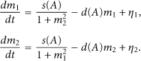
Now let us explain the dynamics of mRNA concentrations following the attractor selection model. An attractor is a stable state, where a nonlinear dynamic system reaches after an arbitrary initial state. When the activity A is high, the nonlinear dynamic system formulated by the above equations has one attractor where $m_1=m_2=m^{*}$ . Here, $m^{*}$ is a constant and larger than one. When the sufficient nutrients are available, a cell grows well. Thus, a cell stays at the attractor and generates either one of two nutrients. Next, we assume that the environment lacks the nutrient, which a cell does not synthesize. Since it does not have the sufficient nutrient to grow, the activity decreases. When the activity becomes low, there appears two attractors, that is, $m_1=m^{*}$ and $m_2=1/m^{*}$ , or $m_1=1/m^{*}$ and $m_2=m^{*}$ , where either one of mRNA concentrations is higher than the other. Since the first two terms of the right side of (1) are multiplied by the activity, potential of attractors are shallow and dynamics is dominated by the noise terms. Consequently, $m_1$ and $m_2$ begin to change at random. When the mRNA concentration of the missing nutrient occasionally becomes large in a cell, the activity slightly increases as the cell can live better. The increase in the activity makes the potential of the attractor deeper and the state of a cell moves toward the attractor by entrainment. The activity further increases accordingly, and the influence of noise becomes smaller. Eventually, the state of a cell reaches an appropriate attractor and stays there stably as far as the nutrient condition does not change.

The attractor selection model is a kind of metaheuristics of optimization problem with dynamically changing given conditions. In the model, possible solutions are defined as attractors of the dynamic system by stochastic differential equations. An objective function to maximize is defined as the activity. In the biological case, a bacterial cell adaptively selects one of solutions, that is, synthesis of either one of two nutrients, so that the cell can maximize its growth rate according to the environmental nutrient condition. In our application of the attractor selection model to coverage control, a sensor node selects one of two states, that is, monitor around or sleep, to maximize the activity defined as the degree of coverage in the target region.

4. Attractor Selection-Based Coverage Control

In this section, we first outline the basic behavior of our proposal. Then, we describe the attractor selection model adopted in our proposal and the definition of the activity in coverage control. Finally, we describe the detailed behavior of sensor nodes in our proposal.

4.1. Overview of Our Proposal

In this paper, we consider a periodic monitoring application, where a sink collects sensing data from sensor nodes at regular intervals as illustrated in Figure 1. We refer to the interval as data gathering interval and the beginning of data gathering as timing of data gathering. We define the duration from the nth timing of data gathering until just before the $(n+1)$ th timing of data gathering as the nth round.

Figure 1

Overview of our proposal.

At each timing of data gathering, each sensor node, which was active in the preceding round, transmits a message to a sink by single or multihop communication. A message consists of sensing data and the information for the sink to estimate the degree of coverage of the target region. Since we focus on coverage control, we do not assume any specific data-gathering mechanism to collect sensing data from sensor nodes. We also assume that the connectivity is maintained when the sufficient coverage is achieved [7]. Using received messages, a sink evaluates the degree of coverage of the target region. The way to evaluate the degree of coverage depends on the requirement of application and the information that sensor nodes can provide. When any localization mechanism is available at sensor nodes, the coverage is estimated based on the relative or absolute location of sensor nodes. An identifier of objects that a sensor node monitors is also useful information when a sink knows locations of the objects in the target region. In this case, each sensor node does not need to know its own location. From the degree of coverage, a sink derives the activity.

Then, a sink disseminates the activity information over a wireless sensor network by using any efficient dissemination mechanism, for example, flooding, gossiping, or tree-based. Not only sensor nodes that are active in the preceding round but also one whose sleep timer expires at the timing of data gathering receives the activity. Sensor nodes that receive the activity decide whether to be active or sleep using the attractor selection model-based state selection mechanisms described below. If a sensor node decides to be active, it starts monitoring its surroundings. Otherwise, the sensor node sets its sleep timer at multiples of data-gathering interval and sleep immediately.

4.2. Extended Attractor Selection Model

In our proposal, we use the following attractor selection model, which is introduced in [11] for adaptive ad hoc network routing:

$\begin{array}{c}\frac{d{m}_1}{dt}=\frac{\text{syn}\left(\alpha \right)}{1+m_2^2}-\mathrm{deg}\left(\alpha \right)m_1+{\eta }_1,\\ \frac{d{m}_2}{dt}=\frac{\text{syn}\left(\alpha \right)}{1+m_1^2}-\mathrm{deg}\left(\alpha \right)m_2+{\eta }_2,\\ \text{syn}\left(\alpha \right)=\alpha \times \left(\beta \times {\alpha }^{\gamma }+{\phi }^{*}\right),\\ \mathrm{deg}\left(\alpha \right)=\alpha .\end{array}$

(2)

This model has two attractors, that is, $m_1>m_2$ or $m_2>m_1$ . β (>0) is a parameter related to the stability of attractor and γ (>0) is a parameter related to the speed of convergence. ${\phi }^{*}$ is a constant for the dynamic system to have stable attractors, and we use $1/\sqrt{2}$ . $\alpha \mathrm{\hspace{0.17em}\hspace{0.17em}}(1\ge \alpha \ge 0)$ is the activity derived from the degree of coverage. The derivation of the activity will be explained in the next section.

4.3. Derivation of Activity

In our proposal, as stated in Section 4.1, any estimation algorithm of the degree of coverage can be adopted. In this paper, we consider the following derivation for the sake of easy implementation and comparison. First, the target region is divided into small regions of $1\hspace{0.17em}[\text{m}]\times 1\hspace{0.17em}[\text{m}]$ , which is called patch. In the target region of $x_t\hspace{0.17em}[\text{m}]\times y_t\hspace{0.17em}[\text{m}]$ , a patch at the column $x\mathrm{\hspace{0.17em}\hspace{0.17em}}(x_t\ge x\ge 1)$ and the row $y\mathrm{\hspace{0.17em}\hspace{0.17em}}(y_t\ge y\ge 1)$ is indicated by $(x,y)$ . The degree of coverage $C\mathrm{\hspace{0.17em}\hspace{0.17em}}(x,y)$ of patch $(x,y)$ is approximated by the number of active sensor nodes whose sensing area covers a center of patch $(x,y)$ .

Guaranteeing any point of the target region to be monitored by k active sensor nodes is called k-coverage. When an application requires k-coverage, the sensing ratio $S\mathrm{\hspace{0.17em}\hspace{0.17em}}(1\ge S\ge 0)$ of the whole target region is derived by the following equation:

$\begin{array}{c}S=\frac{\left|\left\{\left(x,y\right)\mid C\left(x,y\right)\ge k\right\}\right|}{x_t{y}_t}.\end{array}$

(3)

The sensing ratio S does not take into account the excess and deficiency in monitoring, that is, whether a patch is in the sensing area of more or less than k active sensor nodes. Therefore, coverage control using the sensing ratio S as the activity α leads to the waste of energy or deficient coverage. To solve this problem, we formulate the excess and deficiency ratio $E\mathrm{\hspace{0.17em}\hspace{0.17em}}(\ge 1)$ for the whole region:

$\begin{array}{c}E=\frac{{\sum }_{i=1}^{x_t}{\sum }_{j=1}^{y_t}\left|C\left(i,j\right)-k\right|}{x_t{y}_t}+1.\end{array}$

(4)

Then, the activity α for the whole target region is derived as follows:

$\begin{array}{c}\alpha =\frac{S}{\max \left\{1,wE\right\}},\end{array}$

(5)

where larger $w\mathrm{\hspace{0.17em}\hspace{0.17em}}(1\ge w>0)$ leads to more efficient control with less active sensor nodes, but it becomes difficult for sensor nodes to reach solutions, which are deficient or redundant coverage. Operator “max” is introduced to prevent the activity from exceeding one. We call the activity derived in (5) the global activity.

For fine-grained control, we can also define the area activity using the sensing ratio per small areas of the target region. In this case, the target region is divided into some subareas of $x_s\hspace{0.17em}[\text{m}]\times y_s\hspace{0.17em}[\text{m}]$ , where $x_s$ and $y_s$ are divisors of $x_t$ and $y_t$ . A subarea at the column x and the row y is indicated by $(x,y)$ , where $x_t/x_s\ge x\ge 1$ and $y_t/y_s\ge y\ge 1$ . The sensing ratio $S\prime (x,y)$ of subarea $(x,y)$ is derived by the following equation:

$\begin{array}{cc}\hfill S^{\prime }\left(x^{\prime },y^{\prime }\right)& =\left|\{\left(x,y\right)\right|C\left(x,y\right)\ge k,\hfill \\ \hfill & \hspace{1em}\hspace{1em}\left(x^{\prime }-1\right)x_s+1\le x\le x^{\prime }{x}_s,\hfill \\ \hfill & \hspace{1em}\hspace{1em}\left(y^{\prime }-1\right)y_s+1\le y\le y\prime y_{\text{s}}\}|/x_s{y}_s.\hfill \end{array}$

(6)

We formulate the excess and deficiency ratio $E\prime (x,y)\mathrm{\hspace{0.17em}\hspace{0.17em}}(\ge 1)$ for the subarea $(x,y)$ as follows:

$\begin{array}{c}E\prime (x,y)=\frac{{\sum }_{i=\left(x-1\right)x_s+1}^{x{x}_s}{\sum }_{j=\left(y-1\right)y_s+1}^{y{y}_s}\left|C\left(i,j\right)-k\right|}{x_s{y}_s}+1.\end{array}$

(7)

Then, the activity $\alpha \prime (x,y)$ of the subarea $(x,y)$ is given as follows:

$\begin{array}{c}{\alpha }^{\prime }\left(x,y\right)=\frac{S^{\prime }\left(x,y\right)}{\max \left\{1,w{E}^{\prime }\left(x,y\right)\right\}}\end{array}.$

(8)

The activity derived by (8) is called the area activity. In the case of the area activity-based control, a sink evaluates all area activities $\alpha \prime (x,y)$ in (8), and a message from a sink contains all area activities. A sensor node uses the area activity of a subarea in which the sensor node is considered to be located. It implies that a sensor node with inaccurate location information uses the area activity of an inaccurate subarea.

4.4. Node Behavior

A sensor node has three states, that is, active, sleep, and intermediate as illustrated in Figure 2. In each state, a sensor node behaves as follows.

Figure 2

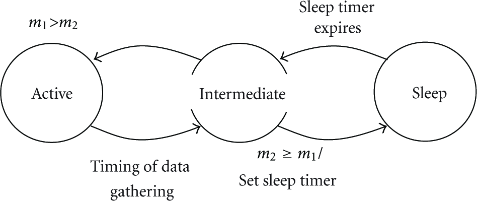
State diagram of our proposal.

4.4.1. Active State

A sensor node monitors its sensing area by turning and keeping sensor modules on and transceiver modules off for the fixed period $I_s$ (>0) [s], which is called sensing interval. When the timing of data gathering arrives, a sensor node turns on transceiver modules and sends sensing data toward the sink. Then, it moves to the intermediate state.

4.4.2. Sleep State

A sensor node turns and keeps all modules off to save its battery. When a sleep timer expires, a sensor node turns on transceiver modules and moves to the intermediate state.

4.4.3. Intermediate State

A sensor node waits for receiving a feedback message from the sink during the fixed period $I_w$ (>0) [s], called intermediate interval. The feedback message contains the activity α, which reflects the degree of coverage. The node evaluates two equations in Section 4.2 to update $m_1$ and $m_2$ using the received activity. In this paper, we assume that above-mentioned transactions are finished within the constant time $I_w$ . Using updated $m_1$ and $m_2$ , sensor nodes select the next state as follows. In case of $m_1>m_2$ , the sensor node moves to the active state. On the other hand, in case of $m_2\ge m_1$ , the sensor node sets its sleep timer as $I_s+l\times (I_s+I_w)$ and moves to the sleep state. $l\mathrm{\hspace{0.17em}\hspace{0.17em}}$ (>0) is a control parameter which is randomly chosen with uniform distribution between 0 and 4 to avoid synchronous behavior of sensor nodes. $I_s+I_w$ corresponds to the data-gathering interval introduced in Section 4.1.

Next, we briefly explain how a sensor node behaves in message transmission in simulation. In the case of a sensor node which was in the active state in the preceding round, it participates in both data gathering and feedback dissemination as illustrated in Figure 3. At the end of active period $I_s$ , the timing of data gathering comes. Although mechanisms of data gathering and feedback dissemination are out of scope of this paper, here we consider a tree-based routing. A sensor node located at i-hop from a sink receives messages from its child sensor nodes and aggregates their sensing data with its own. Then, it sends a message containing aggregated sensing data to its parent sensor node located at $(i-1)$ -hop from a sink and moves to the intermediate state.

Figure 3

Behavior of sensor nodes on i-hop.

During feedback dissemination, a sensor node located at i hop from a sink first receives a feedback message from its parent sensor node during the intermediate interval $I_w$ . Then, it broadcasts the message to its child sensor nodes located at $(i+1)$ -hop from a sink and determines the next state. On the contrary, when a sensor node located at i-hop from a sink was in the sleep state in the preceding round, it does not send sensing data. It wakes up at the timing of data gathering and immediately moves to the intermediate state. Next, it receives a feedback message from its parent sensor node, which was in either of the active or sleep state in the preceding round. Then, it forwards the message to its child sensor nodes and makes a decision on the next state.

4.5. Advantages of Our Proposal

Our proposal have advantages over existing protocols, which require a sensor node to obtain the information of neighbor sensor nodes, that is, location and state. First, our proposal is more robust against the inaccuracy of location information and the irregularity or uncertainty of sensing area than others. In our proposal, a sensor node only requires the degree of coverage of the whole target region or the located area. Even if the derivation of the degree of coverage at a sink uses location information of sensor nodes, the influence of localization error can be mitigated by considering the degree of coverage over the whole target region or the area of a certain size.

Second, our proposal requires less energy in coverage control than others. In other existing proposals, so that a sensor node can appropriately determine the next state using a geometric algorithm, it has to collect sufficient amount of information by receiving many messages from neighbor sensor nodes. Although a sensor node only needs to broadcast a message once to inform neighbor sensor nodes of its information, such message exchanges must be done in addition to regular message transmission for data gathering. On the other hand, our proposal only requires a sensor node to obtain the activity for selecting its sensing state. A sensor node only needs to transmit one message for data gathering and one more for feedback dissemination. Therefore, a sensor node can effectively turn off its transceiver for longer duration than others. These advantages of our proposal will be proved by simulation in the next section.

5. Simulation Experiments

In this section, we first explain error models, that is, localization error and shape error. Simulation results follow to compare our proposal with CCP in terms of the sensing ratio, the number of active sensor nodes, the redundancy ratio, the contribution ratio, and the energy consumption.

5.1. Localization Error

Based on [12], we consider a simple model of localization error. The amount of error is uniformly distributed between $-u$ and u, where u is the maximum error in meter. Then, erroneous coordinates of a sensor node at geographical coordinates $(x,y)$ is given at random in the area of $(x-u,y-u)$ as the left bottom corner and $(x+u,y+u)$ as the right top corner.

In our proposal, a sink evaluates the global or area activity with wrong location information received from neighbor sensor nodes. Therefore, the activity notified to sensor nodes is different from the actual degree of coverage. On the other hand, a sensor node with CCP calculates intersections of sensing areas based on wrong location information. Therefore, the $K_s$ -Eligibility algorithm would give a wrong answer.

5.2. Shape Error

Since there is no model of the irregularity of sensing area, we adopt the model of the irregularity of radio propagation introduced in [13]. RIM (Radio Irregularity Model) models the variation in the received signal strength under the influence of heterogeneous energy loss. In wireless communication, the signal strength decreases in accordance with the distance from the transmitter. The following is the commonly used model to estimate path loss L [dBm] [14]:

$\begin{array}{c}L=C+10n{\mathrm{\hspace{0.17em}\hspace{0.17em}}\log }_{10}d,\end{array}$

(9)

where C is a constant and n expresses the quality of transmission path. Parameter d is the distance between the transmitter and the receiver. Then, RIM introduces the irregularity in path loss as

$\begin{array}{c}R=T-\text{DOI}\hspace{0.17em}\text{Adjusted}\hspace{0.17em}\text{Path}\hspace{0.17em}\text{Loss}+F,\\ \text{DOI}\hspace{0.17em}\text{Adjusted}\hspace{0.17em}\text{Path}\hspace{0.17em}\text{Loss}=L\times K_i.\end{array}$

(10)

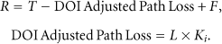
R represents the received signal strength and T corresponds to the transmission power. F corresponds to the fading effect. $K_i$ implements the difference in path loss at the ith degree. $K_i$ is given by the following equation:

$K_i=\{\begin{array}{cc}1,\hfill & \text{if}\mathrm{\hspace{0.17em}\hspace{0.17em}}i=0,\hfill \\ K_{i-1}\pm r\text{DOI},\hfill & \text{if}\mathrm{\hspace{0.17em}\hspace{0.17em}}360>i>0\wedge i\in N,\hfill \end{array}$

(11)

where $\mathrm{\hspace{0.17em}\hspace{0.17em}}\text{DOI}\ge |K_0-K_{359}|$ .

Here, $\text{DOI}$ (degree of irregularity) is the coefficient of the irregularity. r is a random number following the Weibul distribution.

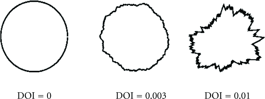
For example, we depict the impact of different DOI in Figure 4. Each shape shows the border of region where the received signal strength exceeds a certain threshold. As can be seen, DOI = 0 gives a circular shape. As DOI increases, the shape becomes more irregular. We first set parameters of RIM appropriately to obtain the regular circle shape of the desired sensing radius and then change DOI to see the influence of irregularity in simulation experiments.

Figure 4

Irregular sensing area.

5.3. Energy Model

We define the energy model based on MICAz [15, 16]. CPU consumes 8 [mA] when it is on and 15 [uA] when it is off. A transceiver module consumes 19.7 [mA] in listening a channel and receiving a message and 17.4 [mA] in transmitting a message. A sensor module consumes 10 [uA] when it is on and 0 [uA] when it is off. When a sensor module monitors objects, CPU is activated as well. We assume that a sensor node runs on two AA batteries of 3 [V].

As explained in Section 4.4, we consider a tree-based routing for data gathering and feedback dissemination. In data gathering, a sensor node receives sensing data from its child sensor nodes, generates the aggregated data of the same size of a single sensing data, and sends it to a parent sensor node. In disseminating feedback messages, a sensor node receives a message containing the activity from its parent sensor node and broadcasts it to all child sensor nodes.

5.4. Simulation Setting

We distribute about 10,000 sensor nodes in the square target region. A sink is located in the center of the target region. In the case of the global activity-based control, 10,000 sensor nodes are randomly deployed in the target region of $500\hspace{0.17em}[\text{m}]\times 500\hspace{0.17em}[\text{m}]$ . In the case of the area activity-based control, we first set the size of a subarea and then determine the size of the target region as the multiple of a subarea around 500 [m], while keeping the density 0.04 [node/m²]. For example, when the size of subarea is $15\hspace{0.17em}[\text{m}]\times 15\hspace{0.17em}[\text{m}]$ , 10,404 sensor nodes are distributed in the target region of $510\mathrm{\hspace{0.17em}\hspace{0.17em}}[\text{m}]\times 510\mathrm{\hspace{0.17em}\hspace{0.17em}}[\text{m}]$ . An application requires 1, 2, or 3-coverage ( $k=1$ , 2, or 3). Data-gathering interval $(I_s+I_w)$ is set at 10 [s]. Sensing interval $I_s$ is 9 [s] and wakeup interval $I_w$ is 1 [s]. At the beginning of a simulation run, all sensor nodes are in active state.

In our proposal, both $m_1$ and $m_2$ are initialized to 1 and the initial activity is initialized to 0. Parameter, β and γ are set at 2.5 and 1.2, respectively. Weight w is set at 0.5. The parameter l of rounds of sleep state in our proposal is randomly chosen between 0 and 4 with uniform distribution. These parameters are selected through preliminary experiments. In CCP, HELLO interval, SLEEP, WITHDRAW, JOIN, and LISTEN timers are set at 1 [s], 10 [s], 1 [s], 1 [s], and 1 [s], respectively. Regarding details of these parameters, refer to [7]. For the purpose of comparison, we define ACTIVE and JOIN state of CCP as active state.

The communication range $R_c$ is set at 20 [m]. We use our own simulator and we assume the ideal communication environment; that is, there is no loss or delay of message. The shape of sensing area is a circle of radius $R_s=10$  [m] and identical among sensor nodes under the condition without shape error. In our proposal, a sink assumes the circular sensing area with radius 10 [m] and believes the location information reported by sensor nodes in derivation of the activity. In CCP, intersection points between borders of sensing areas of neighbor sensor nodes are calculated under the assumption that there is neither localization error nor shape error. For evaluation of the tolerance to localization error, we change the maximum location error u from 0 [m] to 10 [m], for example, GPS-based localization. For evaluation of the tolerance to shape error, we change DOI from 0 to 0.03.

5.5. Performance Measures

As performance measures, we use the number of active nodes N, the contribution ratio B, the redundancy ratio U, and the energy consumption O. The contribution ratio B indicates the degree of contribution of an active sensor node to coverage. B is derived as

$\begin{array}{c}B=\frac{M\times S}{N}\hspace{0.17em}\left[{\text{m}}^2\right],\end{array}$

(12)

where M [m²] is the size of target region and S is the sensing ratio derived by (3) with the accurate coordinates and sensing area. Therefore, the contribution ratio represents the average area that an active sensor node is responsible for monitoring. The larger contribution ratio means that sensor nodes are more efficiently monitoring.

Next, we define the redundancy ratio U as the averaged extra degree of coverage per patch for achieving k-coverage. The redundancy ratio is derived as

$\begin{array}{c}U=\frac{\sum _{i=1}^{x_t}\sum _{j=1}^{y_t}Z\left(C\left(i,j\right)\right)}{\left|\left\{\left(x,y\right)\mid C\left(x,y\right)\ge k\right\}\right|},\\ Z\left(x\right)=\{\begin{array}{cc}x-k+1,\hfill & \text{if}\mathrm{\hspace{0.17em}\hspace{0.17em}}x\ge k,\hfill \\ 0,\hfill & \text{if}\mathrm{\hspace{0.17em}\hspace{0.17em}}x<k,\hfill \end{array}\end{array}$

(13)

where the target region is $x_t\hspace{0.17em}[\text{m}]\times y_t\hspace{0.17em}[\text{m}]$ and the coverage $C(x,y)$ of patch $(x,y)$ is approximated by the number of active nodes that has a center of patch $(x,y)$ in its own sensing area. Therefore, the larger redundancy ratio means that too many nodes are in the active state.

Finally, the energy consumption O is derived using our energy model described in Section 5.3. We take into account state-dependent energy consumption and energy consumed in message transmission and reception. We should note here that the overhead related to management of location information is not considered in the evaluations. First, we assume that a sink obtains identifiers and location-related information from all sensor nodes in advance. We further assume that both of CCP and our proposal adopt the same localization technique. Messages sent from a sensor node contain its identifier, whose size is small enough. As a result, the amount of overhead regarding management of location information is almost the same among CCP and our proposal, and the difference is negligible. Influences of inaccuracy in location information are taken into account in the energy consumption O, since inaccurate location information affects states of sensor nodes and the amount of message transmission.

5.6. Basic Evaluation

First we compare our proposal with CCP under the ideal environment, where there is neither localization error nor shape error. In Figure 5, the x-axis indicates the width and height of a subarea, that is, $x_s$ and $y_s$ , for the area activity-based control. $x_s=y_s=500$  [m] corresponds to the case of the global activity-based control where the target region is not divided into any subarea. The y-axis shows the sensing ratio derived by (3). When there is no error, CCP accomplishes the sensing ratio S of 1.0 for $k=1$ , 2, and 3 as shown in Figure 5(a).

Figure 5

Comparison without errors.

Under the ideal environment, sensor nodes can accurately estimate the degree of coverage inside sensing areas of themselves. Figure 5(b) shows that the percentage of active sensor nodes with CCP increases almost in proportional to the required coverage. In spite of a deterministic and geometric algorithm of CCP, the redundancy ratio is higher than 2 and up to 3.2 as shown in Figure 5(c). Even if an uncovered area inside a sensing area of a sensor node is small, a sensor node becomes in active state to cover the area. This results in the redundant coverage of the other area which is already covered. However, such redundancy is unavoidable for the irregularity of deployment of sensor nodes and the shape of sensing area.

Compared to CCP, the sensing ratio with our proposal is lower especially when the size of subarea is large as shown in Figure 5(a). Our proposal adopts the metaheuristic algorithm, that is, attractor selection model, to find a solution. As such, the size of search space affects the optimality of the found solution. In case of the global activity-based control, the number of combinations of state of sensor node is as large as 2¹⁰⁰⁰⁰. In addition, a state of a sensor node does not influence others very much. Therefore, our proposal often falls into local optimal. However, as the sizes of subareas decreases, the sensing ratio of our proposal approaches 1. When the size of subarea is smaller, the number of sensor nodes per subarea decreases. As a result, the size of solution space becomes smaller and there appears stronger interdependency among state of sensor nodes. In other word, with the smaller size of subarea, sensor nodes can find better solution, which has higher sensing ratio and less redundancy ratio. In general, when a sensor node selects the active state, it increases both of the sensing ratio and the redundancy ratio. When the sensing ratio is low, an increase in the sensing ratio increases the activity more than the decrease caused by increased redundancy ratio. It is a reason that there are more active sensor nodes with smaller subareas in Figure 5(b) for $k=2$ and 3. On the other hand, when k is 1, even with a small subarea, it is hard for an additional active sensor node to increase the sensing ratio, which is already high enough. Therefore, the coverage control moves toward reducing the redundancy ratio to increase the activity as shown in Figure 5(c).

Regarding the contribution ratio, a smaller subarea leads to the higher contribution ratio. As shown in Figure 5(d), when k is 2 or 3, our proposal can achieve higher contribution ratio than CCP in any size of subarea. On the contrary, when k is 1, CCP achieves higher contribution ratio than our proposal in almost all size of subarea. When $x_s$ and $y_s$ are 500 [m] and k is 1, 2, or 3, about 22 percent of sensor nodes becomes active state. In comparison with CCP, in case of $k=1$ , the number of active sensor nodes is redundant to achieve the perfect 1-coverage ( $k=1$ ). In addition, due to the low optimality of the found solution, our proposal achieved less sensing ratio than CCP. Because of low sensing ratio and redundant active sensor nodes, our proposal achieves less contribution ratio than CCP. Using smaller subareas, our proposal can find better solutions, that is, achieving higher sensing ratio by less active sensor nodes. In particular, when k is 1 and $x_s$ and $y_s$ are 5 [m], the number of active sensor nodes in our proposal drops to below CCP, and the magnitude relation of contribution ratio is reversed. In addition, when k is 2 and 3, the number of active sensor nodes increases unlike when k is 1, but the sensing ratio also more increases. Therefore, higher contribution ratio can be achieved as subareas become smaller.

5.7. Influence of Localization Error

In this section, we compare CCP and two variants of our proposal, that is, the global activity-based control and the area activity-based control whose subarea size is set at $10\hspace{0.17em}[\text{m}]\times 10\hspace{0.17em}[\text{m}]$ , under the influence of localization error. For the sake of argument about the origin of the error tolerance of our proposal, we show the results of CCP with the center-point control in addition to the results of original CCP. We call the original CCP “distributed-CCP” and the CCP with the center-point control “centralized-CCP”. In the centralized-CCP, a sink collects the sensing state and location-related information from all sensor nodes and conducts the $K_s$ -Eligibility algorithm for each of the sensor nodes. Then, the determined state is sent back to each sensor nodes. To ignore the influence of shape error, DOI is set at zero. Figures 6 and 7 summarize results averaged over 10 simulation runs.

Figure 6

Influence of localization error (global activity).

Figure 7

Influence of localization error (area activity).

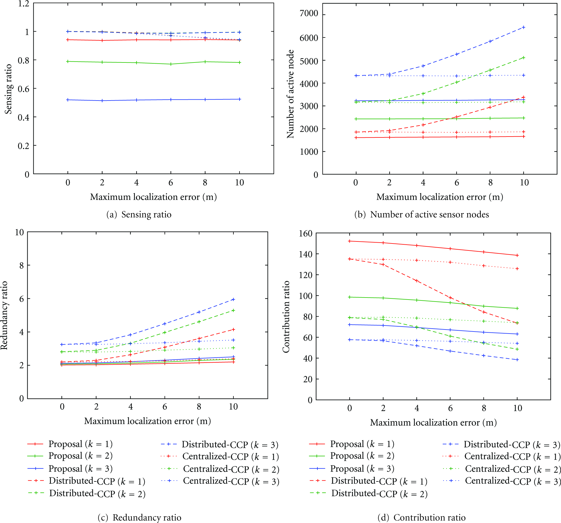
Figure 6(a) shows the average sensing ratio S of the global activity-based control against the different degree u of localization error. In the figure, it is obvious that neither our proposal nor distributed-CCP is affected by localization error. In our proposal, a sink calculates the activity from collected sensing data. Since the effect of localization error is averaged over the whole region, the derived activity is not seriously affected by localization error. On the contrary, distributed-CCP uses geometric and deterministic algorithm, and as such state selection heavily depends on the accuracy of location information. Nevertheless, distributed-CCP keeps the high sensing ratio. The reason is that localization error and wrong state selection are compensated by the increased number of active sensor nodes and the higher redundancy as shown in Figures 6(b) and 6(c).

In CCP, localization errors contribute to both of increase and decrease in the number of active nodes. When a sensor node wrongly considers that a neighbor sensor node is far and there is no overlap between their sensing areas by localization error, it is likely to become active to monitor intersections which seem to be uncovered. At the same time, localization error makes a sensor node consider a further neighbor to be located close. Consequently, the affected node is likely to move to the sleep state. In the case of the distributed-CCP, a decision of a sensor node is affected only by neighbor sensor nodes within its communication range. From results of the distributed-CCP in Figure 6(b), localization error results in the increase more than the decrease. On the contrary, in the case of the centralized-CCP, a sensor node is further affected by localization error of a sensor node whose actual location is out of its communication range. The actual sensing area of such a distant sensor node does not overlap with the sensing area of the sensor node. Therefore, even if the distant sensor node is considered to be located further by localization error, it does not influence a decision of the sensor node at all. However, when the sensor node considers the distant sensor node is located closer to itself by localization error, it would move to the sleep state. As a result, the number of active sensor nodes becomes smaller than that of the distributed-CCP. Since the increase and decrease are occasionally balanced for uniformly random distribution of sensor nodes, the number of active sensor node becomes constant against localization errors.

As a result, the redundancy ratio with the centralized-CCP becomes smaller than the distributed-CCP (Figure 6(c)), and the centralized-CCP is more prone to the localization error than the distributed-CCP in terms of the sensing ratio (Figure 6(a)). Similarly, in our proposal, the derived activity is not also seriously affected by localization error by averaging error over the whole region, we can achieve the similar performance without increasing the number of active sensor nodes.

To evaluate the efficiency of coverage control, Figure 6(d) shows the contribution ratio B against the different degree of localization error. As can be expected from Figure 6(b), the contribution ratio of distributed-CCP decreases as the maximum localization error increases. For example, when an application requires 1-coverage ( $k=1$ ), the global activity-based control accomplishes more efficient coverage control than CCP with maximum localization error u of 6 meters or more. When an application requires 2 or 3-coverage ( $k=2$ or 3), our proposal always outperforms both the distributed-CCP and the centralized-CCP in terms of the contribution ratio. When we divide the target region into subareas whose size is 10 [m] and apply the area activity-based control, we can achieve higher sensing ratio than the global activity-based control. Especially, in the case of $k=1$ , the similar degree of sensing ratio can be achieved with the smaller number of active sensor nodes. Moreover, the area activity-based control outperforms both distributed-CCP and centralized-CCP in terms of the contribution ratio while the sensing ratio is sufficiently high such as more than 0.8.

However, the sensing ratio gradually decreases as the localization error increases. In comparison with the global activity-based control, the redundancy ratio is lower and the contribution ratio is higher with the area activity-based control (compare Figure 6(c) with Figure 7(c), Figure 6(d) with Figure 7(d)). It implies that an uncovered patch has less chance to be covered by a nearby active sensor node than with the global activity-based control. However, even if there is the high localization error, the area activity-based control can achieve the sensing ratio similar to or better than the global activity-based control.

From the above results, we can conclude that our proposals are more robust than distributed-CCP. Although centralized-CCP exhibits the similar robustness in the number of active nodes to our proposal due to the center-point control, our proposal is superior to centralized-CCP. Further discussions will be given in Section 6. Although distributed-CCP can maintain sensing ratio close to one against localization error, the number of active sensor nodes considerably increases. It depletes batteries and shortens the lifetime of a sensor network. Although sensing ratio is slightly lower with the area activity-based control than distributed-CCP even without localization error, the number of active sensor nodes do not change much, and we can expect the similar lifetime under the influence of localization error, which is quite common in the actual environment. When we consider such applications that do not always require sensing ratio of 100%, for example, precision agriculture and environmental monitoring, our proposal is more practical and useful than distributed-CCP.

5.8. Influence of Shape Error

Figure 8 evaluates the influence of shape error on the sensing ratio under the condition without localization error. As shown in the figure, the sensing ratio decreases independently of protocols, and their order does not change against the degree of irregularity. When there are shape errors, a patch considered to be inside the ideal and circular sensing area of an active sensor node is not always inside the actual and irregular sensing area. It leads to decreasing the sensing ratio. On the other hand, even if a patch is covered by a distant active sensor node whose actual sensing area contains the patch, it does not contribute to the sensing ratio calculated at a sensor node or a sink. It is because another node whose circular sensing area contains the patch decides to become in active state for insufficient coverage from a viewpoint of the sensor node and the patch becomes covered anyway. As a result, the shape error causes deterioration of sensing ratio.

Figure 8

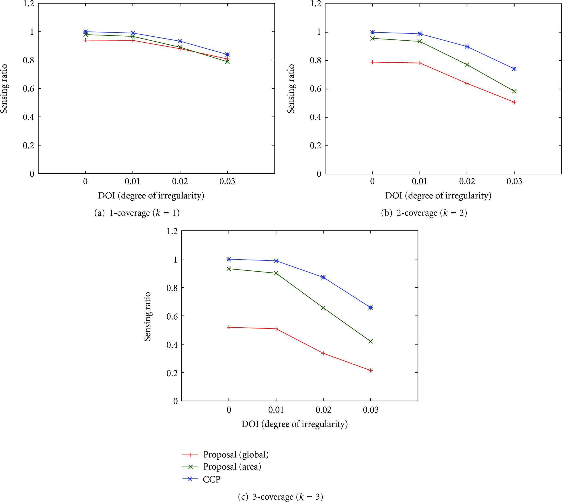
Influence of shape error.

5.9. Evaluation of Energy Consumption

Finally, we evaluate energy consumption of our proposal and CCP. Figure 9 shows the averaged energy consumption per sensor node over 10 simulation runs against time for cases with and without localization error. Results of our proposal with and without localization error overlap with each other. This is because the number of active sensor nodes does not increase even with high localization error. A reason why the global activity-based control requires more energy than the area activity-based control for $k=1$ , similar energy for $k=2$ , and less energy for $k=3$ is that it requires more, similar number of, and less active sensor nodes for $k=1$ , 2, and 3, respectively, as shown in Figures 6 and 7. On the contrary, in the case of CCP, localization error depletes more energy for the increased number of active sensor nodes (see Figures 6 and 7). For 1-coverage ( $k=1$ ), the amount of energy consumption with localization error becomes 1.35 times as much as that without localization error, whereas the number of active sensor nodes increases by about 1.8 fold.

Figure 9

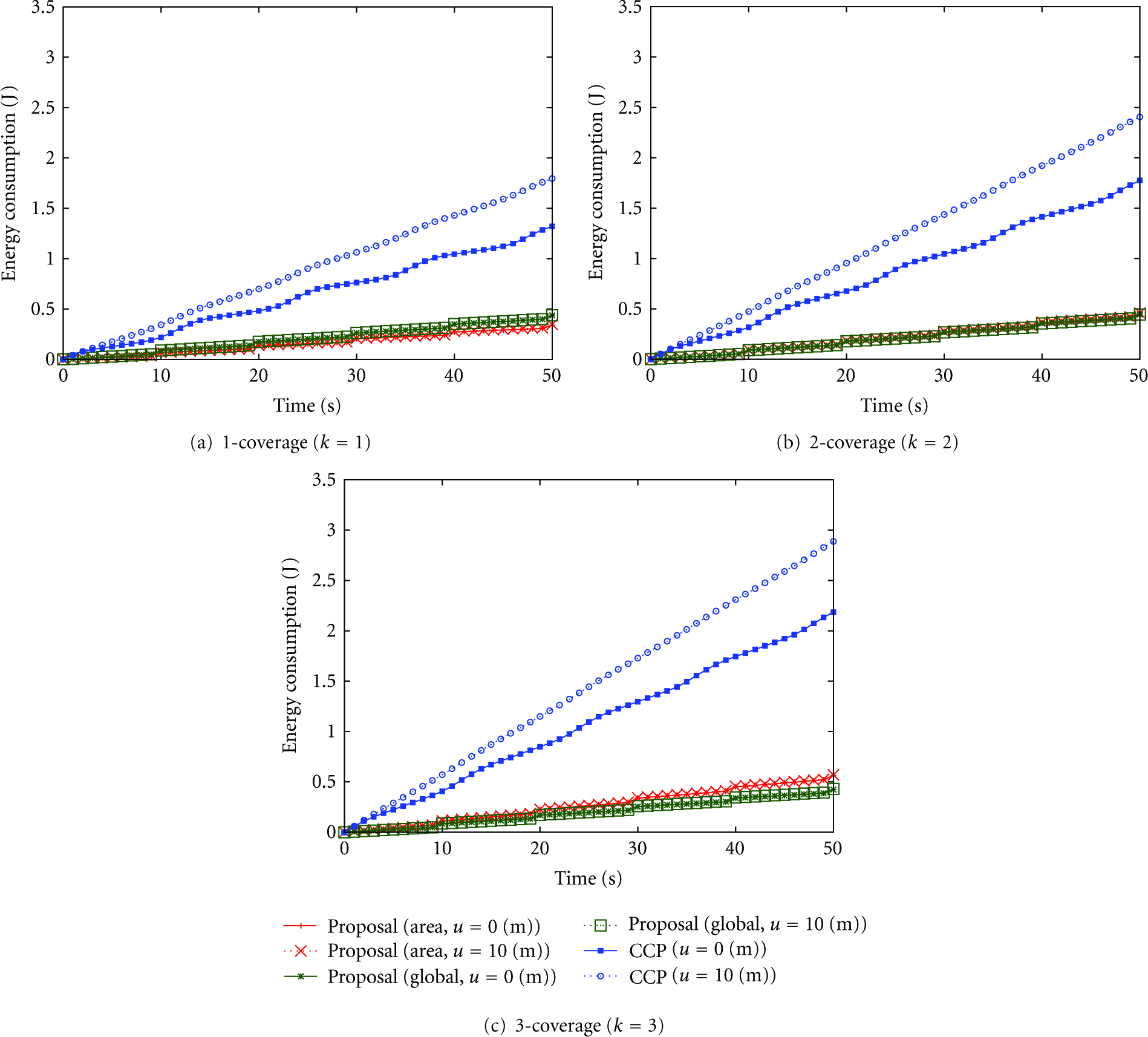
Energy consumption.

Independently of the required coverage, it is apparent that our proposal consumes only between one-sixth and one-third of energy of CCP. The primary reason lies in less communication overhead of our proposal. Our proposal does not involve any additional communication among sensor nodes except for dissemination of activity. Therefore, sensor nodes can turn off transceiver modules except for data gathering and feedback dissemination and hold down energy consumption. On the other hand, CCP consumes energy in the listen mode of transceivers for information exchanges and state transitions. To evaluate the $K_s$ -Eligibility and confirm state transition, a sensor node has to keep a transceiver module listening to a channel for longer duration than our proposal. Furthermore, CCP requires a larger number of sensor nodes to be active than our proposal when there is a large localization error. Because of the smaller energy consumption, our proposals can accomplish the longer lifetime of sensor network than CCP. For example, although the sensing ratio with the area activity-based control is about 0.8 for $k=3$ and $u=10$  [m] as shown in Figure 7(a), the lifetime of a sensor network is about six times as long as that with CCP.

6. Discussion

As seen in the results of centralized-CCP, center-point control leads to the robustness against localization error in the number of active sensor nodes. This results in the higher contribution ratio of the centralized-CCP than that of the distributed-CCP. Since our proposal adopts a kind of center-point control, where the activity, expressing the degree of coverage of the whole region or each subarea, is derived at a sink, they have the similar robustness. However, the center-point control alone is not sufficient to explain the reason of higher performance of our proposal than the CCP-based control schemes. A reason that our proposal can outperform the CCP-based schemes by the smaller number of active sensor nodes is in the bio-inspired algorithm. CCP relies on the deterministic and rigorous algorithm, aiming at the perfect coverage. As a result, many sensor nodes are forced to be active to fully fill out the region with active nodes. For example, a sensor node decides to become the active state to cover a small void, whose size is less than 1/10 of the sensing area. On the contrary, the bio-inspired algorithm is more flexible and relaxed. A single scalar, called the activity, is used to express the degree of coverage of the whole region or each subarea in a rough and vague manner. In addition, each sensor node decides its state stochastically and autonomously. As such, the number of active sensor nodes is efficiently reduced while leaving some, voids are uncovered with our proposal, and the sensing ratio is sacrificed to some extent.

7. Conclusion

In this paper, by adopting the attractor selection model of adaptive behavior of biological systems, we proposed an error-tolerant and energy-efficient coverage control and showed our proposal can achieve the sensing ratio S of up to 0.98 and prolong the life time of the network up to 6 fold by comparison with CCP.

As future research, we plan to conduct more realistic evaluation, where radio communication interferes with each other. CCP will suffer from collisions among control messages and the performance will deteriorate. On the contrary, feedback dissemination will be affected by loss of messages. As a result, some sensor nodes cannot update the activity, and the performance will deteriorate as well. We also need to investigate the influence of parameters of the attractor selection model. Biological models are insensitive to parameter settings in general and it is one of benefits to be inspired by biological systems. We are going to evaluate our proposals with other simulation scenarios.