
Abstract
Near-ground channel characterization is an important issue in most military applications of wireless sensor networks. However, the channel at the ground level lacks characterization. In this paper, we present a path loss model for three near-ground scenarios. The path loss values for each scenario were captured through extensive measurements, and then a least-square linear regression was performed. This indicates that the log-distance-based model is still suitable for path loss modeling in near-ground scenarios, and the prediction accuracy of the two-slope model is superior to that of the one-slope model. The validity of the proposed model was further verified by comparisons between the predicted and measured far-field path losses. Finally, compared to the generic models, the proposed model is more effective for the path loss prediction in near-ground scenarios.
1. Introduction
Wireless sensor networks (WSNs) are an enabling technology for the distributed monitoring of industrial, military, and natural environments [1, 2]. In most military applications, the sensors are placed at the ground level, and their antennas rise a few centimeters above the ground [3, 4]. However, almost all studies to date were based on the assumption that the antennas were placed one meter or more above the ground, which could not accurately capture the behavior of an authentic WSN [3]. It is well known that the signal strength and associated noises are affected by the channel characteristics, which depend on an authentic testing environment. Therefore, the propagation characteristics of near-ground environments are important to system designers for network planning [5, 6].
The rise of WSN applications has prompted the need for a more complete understanding of near-ground propagation channels. In [7], one of the first studies of near-ground wideband channel measurement was conducted in 800–1000 MHz, and eleven indoor or outdoor sites were measured with an antenna height of approximately 15 cm. In [8, 9], another two earlier works related to near-ground RF propagation measurement were carried out for military or emergency applications at the frequency of 915 and 879 MHz, respectively. The authors investigated the scenario of a person lying on the ground attempting to place a call with an antenna very near the ground (several or several tens of centimeters in height). Joshi et al. presented narrowband and wideband channel measurement results at 300 and 1900 MHz for near-ground propagation with characterizing the effect of antenna heights, radiation patterns, and foliage environments [10], but the lowest antenna height was 0.75 m, which was insufficient for an authentic near-ground scenario. Martínez-Sala et al. presented the near-ground channel characterization for WSNs in three outdoor scenarios, validated a two-slope lognormal path loss channel model at 868 MHz, and compared it to the widely used one-slope model [3]. Subsequently, Meng et al. investigated near-ground radio wave propagation in a tropical forest in the VHF and UHF (40, 80, 250, and 550 MHz) bands [11]. The antenna height selected in their measurement campaigns was 2.15 m, which was not the expected case for most WSNs when established in outdoor environments. Other research activities related to near-ground channels included the study of radio wave propagation in a car park at 433 MHz [6] and assessment of indoor or industrial ultrawideband (UWB) channels [4, 5, 12].
As stated above, although attention has recently focused on modeling near-ground propagation channels, few studies investigate propagation in near-ground environments with antenna heights in several centimeters level, especially for the 2.4 GHz band. In this paper, we propose a statistical model for near-ground channels based on extensive measurements.
The initial intention of the work is to assess the coverage capability of a WSN developed for data (pressure or temperature) acquisition in military explosive research. The sensor nodes are fixed on the ground in the explosion field for the testing task, and the antenna height of sensor nodes is set as low as 3 cm to resist physical damage from nearby detonations. It is well known that, due to the proximity of the antenna to the ground, significant performance degradation may occur [3, 4]. So, effective path loss prediction becomes a key issue in system design. In fact, different propagation models should be applied in different environments, but to our knowledge, no appropriate model exists for the near-ground scenario. Therefore, the results of extensive measurements and path loss modeling in the authentic application environment are presented in this paper. For the purposes of comparison, two other representative environments are selected as measurement sites. In all the sites, the same measurement and analysis procedures are applied, and the derived model is validated by far-field measurement data. Finally, the performance of the obtained model is compared with the generic models.
The paper is organized as follows: in Section 2, the scenarios are described in further detail. In Section 3, the measurement methodology is summarized. In Section 4, the measured results and a discussion of each site's results are presented. A path loss model for near-ground radio wave propagation is derived and then compared with the previous models. The summary and conclusions are presented in Section 5.
2. Near-Ground Scenarios
Generally, the target scenario for outdoor WSN application is just above ground level. Sensor nodes with a very low antenna height are placed on the ground randomly or regularly. Near-ground scenario is a complex environment due to reflection, obstruction, and absorption occurring from the ground and vegetation [6, 10]. Channel measurements and modeling are, therefore, a basic necessity for system design. Three different outdoor environments were selected in this work, including a large plaza, a straight sidewalk, and an open grassland (see photographs in Figure 1).
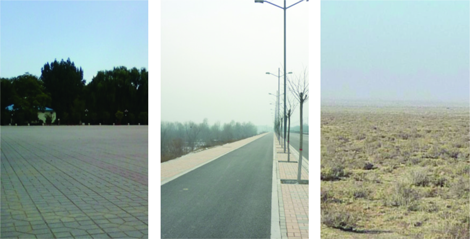
Photograph of the measurement sites.
The first site is located at the school yard of North University of China (NUC). It is a rectangular-shaped site (an area of 115 × 100 m2) bordered by trees and several buildings. The trees are almost equally spaced, with a separation of 2 m, and their trunks have a diameter of no more than 10 cm. The ground is paved with bricks, and the terrain is fairly flat. The second site is a straight sidewalk along with suburban road, and the other side is a large plot of lowland with scattered trees. The sidewalk is paved with pitch and bricks, and the terrain is nearly flat. A line of lampposts are spaced 35 m apart along the sidewalk, and several low trees are nearly equally spaced between the lampposts. The lamppost has a conical profile with a maximum diameter of 20 cm at the base, and the dimensions are comparable to the radio wavelength. The open grassland is the authentic application environment for WSN in testing experiments. The terrain is basically flat, consisting of soil and sand. Most of the areas are covered by vegetation, and a large number of shrubs are scattered in the areas with an average height of approximately 40 cm. Given the low antenna height, this environment can be seen as a non-line-of-sight (NLOS) situation.
Although the terrain is flat, as can be seen from Figure 1, significant attenuation in radio wave propagation will exist due to the very low antenna height. This is further verified in Section 4. Furthermore, each site has different features and thus can be predicted to have its own exclusive propagation characteristics.
3. Measurement Methodology
For the purpose of conducting an experimental channel characterization for path loss assessment, only narrowband measurement trials were carried out. The sensor node had a narrowband RF transceiver working at 2.4 GHz, which was used as a transmitter. The receiver consisted of a portable spectrum analyzer and a laptop computer illustrated in Figure 2. The spectrum analyzer (Agilent N9912A) acquired signal strength data, and the laptop computer was used for data storage. A pair of vertical-polarization omnidirectional antennas with a calibrated gain of 2 dBi were used as transmitting and receiving antennas. Both antennas were connected to the transmitter or receiver by a low-loss coaxial cable. During the measurements, the transmitter sent a carrier of 19 dBm (maximum radiated power for radio range extension) at 2.4 GHz, and the spectrum analyzer was set to this central frequency.

Photograph of the measurement setup.
At each of the three previously mentioned sites, the same methodology was applied. The transmitter was fixed in a position with different antenna heights of 3 cm and 1 m. The receiver was separated from the transmitter by up to 100 m, and the antenna height was varied from 1 to 2 m. Along the straight line followed by the receiver, the samples were collected every meter in a distance of up to 10 meters from the transmitter, and then every 2 meters until the end. At each nominal position, 10 testing points over 10 cm around the central position were selected for spatial averaging, 20 samples were collected at each testing point for time averaging, and 200 samples were acquired in total. In practice, since the sensor nodes do not move, stationary testing points were selected. In addition, there was no moving machinery at the sites during the measurements, and no moving personnel. Therefore, it is reasonable to assume that the measurement environment is stationary, and the channel of interest is slowly time varying [7]. Special attention was paid to various antenna heights in the measurement because the server node (receiver) has an antenna height of about 1–3 m higher than the sensor nodes in practical applications. Also, to compare performance, an antenna height of 1 m was selected as the same case in the measurements for all the sites.
4. Channel Modeling and Analysis
After data collection, 55 datasets were recorded in one measurement campaign, and the raw data in each dataset was examined firstly to eliminate the singular point. In order to obtain a mean value of the measured signal strength, for a nominal position, time averaging for each testing point around the central position was firstly performed, and then spatial averaging was performed among the testing points, which could mitigate the effects of the small-scale fading. Subsequently, the local mean path loss was calculated. Based on the preliminary analysis, it is found that the path loss tends to a linear relation with the log-distance, so the log-distance-based pass loss model can be used for channel characterization. The measured results and the process of modeling are presented in Section 4.1, and the validity of the model is verified with the experimental data in Section 4.2. Two generic models related to the near-ground scenarios are briefly introduced in Section 4.3, and their performances on the path loss prediction are compared with the proposed model.
4.1. Path Loss Modeling
Path loss is a fundamental characteristic of radio wave propagation, which is often used for link budget calculation and determining transceiver ranges [4]. For radio wave propagation in outdoor environments, both theoretical and measurement-based propagation models indicate that the average of received signal power decreases logarithmically with the distance [13, 14]. In this section, the measured path losses versus the log-distance are plotted in Figures 3, 4, and 5 for all the sites, and an approximate linear relation can be found between the path loss and the log-distance. So the linear regression can be used for data fitting, and the process is summarized as follows.

The measured path loss and the regression lines in the plaza. (a)
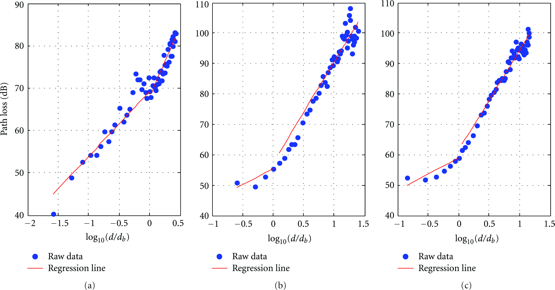
The measured path loss and the regression lines in the sidewalk. (a)

The measured path loss and the regression lines in the grassland. (a)
4.1.1. Linear Regression
Assume that there are m samples at the transmitter-receiver (T-R) separation distance of
one-slope model:

two-slope model:
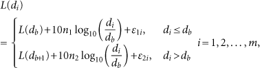
where in (1)
Then, the linear regression can be executed in MATLAB by using the least-square method. Assume that

During the process of regression, the value of
The regression process of the one-slope model is similar to that of the two-slope model. However, the breakpoint does not need to be calculated, and
Finally, in order to examine the goodness of logarithmic fit, two statistical parameters, that is, the residual standard deviation (σ) and the correlation coefficient (

where
The correlation coefficient represents how successful the fit is in explaining the variation of the data. It is defined as the square of the correlation between the measured and the predicted path losses. For the two-slope model, it can be expressed as

Where
The calculation of these two statistical parameters for the one-slope model is similar to that above defined with no breakpoint.
4.1.2. Statistical Parameters
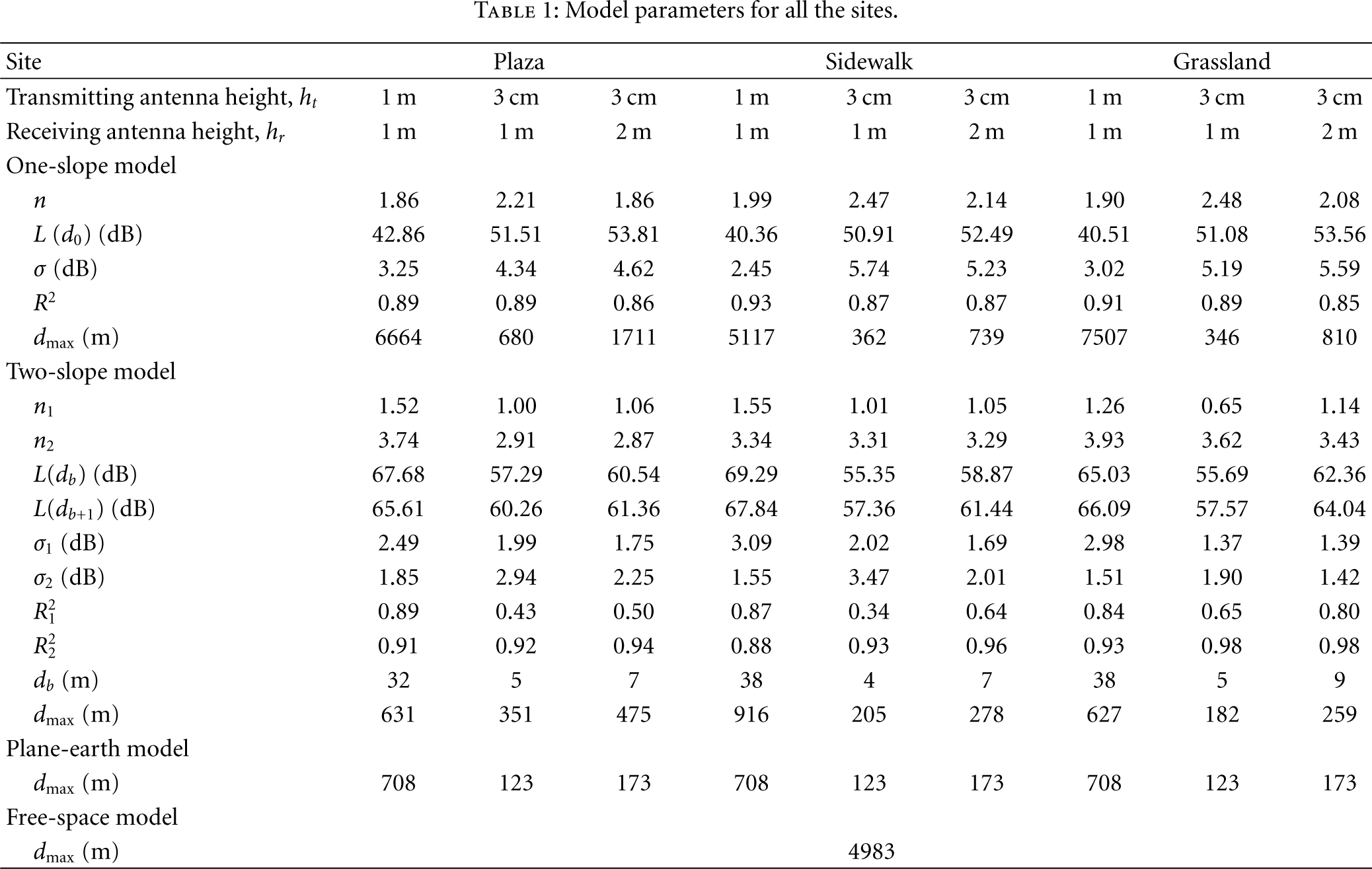
The regression line of the path loss is also drawn for each data set in Figures 3–5, and the key parameters for each model are summarized in Table 1. Figures 3–5 illustrate that the regression line tends to a better fit to the raw data for all the sites, which can be further verified by the statistical parameters in Table 1. It is confirmed consistently in Table 1 that for the two-slope model, the residual standard deviation (
Model parameters for all the sites.
4.1.3. Breakpoint Distance
It is observed from Figures 3–5 that there is a certain breakpoint among each data set which indicates different change rate of the path loss, and intuitively, the breakpoint distance varies in different data sets. In general, when a LOS condition is available, the breakpoint distance can be estimated by [15, 16]

For the three cases, where
4.1.4. Path Loss Exponent
The resulting values of the path loss exponent are also given in Table 1. It is found that, for the one-slope model, the n value is around 2 and varies between 1.86 and 2.48, which corresponds to 18.6–24.8 dB attenuation per decade of distance. Intuitively, this attenuation rate seems low, even compared to the free-space model (
For the two-slope model, Table 1 illustrates that the slope before the breakpoint (
Another phenomenon that should be mentioned is that although the
From Figures 7 and 8, the path loss for the grassland is closer to that of the sidewalk, which seems not to fit well with the authentic environment. This is not surprising, since at 2.4 GHz frequency, the wavelength of the signal is comparable in size with the dimensions of the vegetation. Hence, more forward scattering is caused by the dense vegetation. This forward scattering can counteract the loss due to absorption and attenuation caused by the vegetation, thus the much lower attenuation rate [11]. Moreover, in Figure 7, the difference in path loss between the two sites is further reduced as the
In addition, for a given site, the path loss when
4.2. Verification with the Measured Data
To prove the validity of the proposed model, for the sites of sidewalk and grassland, the path loss for different locations far from the transmitter was measured and then compared with the value predicted by the proposed model. The plaza site was not further measured due to the restriction of area, and the verification could not be carried out. Several typical testing points for the other two sites are presented in Tables 2-3, where
Comparisons between the predicted path loss and the measured path loss in far field for the sidewalk.

Comparisons between the predicted path loss and the measured path loss in far field for the grassland.

4.3. Comparison to the Generic Models
In order to provide a better representation of the proposed model, the performance of the two-slope model is compared with that of the generic models. Due to the flat terrain at all three sites, the free-space model can be compared with the two-slope model. The path loss for the free-space model [18] at 2.4 GHz is given as

where d is the distance between the transmitter and receiver in kilometers.
When the radio wave propagates near the ground with a line-of-sight (LOS) condition, the path loss can be better described by the plane-earth (PE) path loss model rather than the free-space model [10]. The plane-earth path loss model [19] includes antenna heights and the effect of ground reflection, which is given as

where d is the distance between the transmitter and receiver in meters;
The path loss predicted by the two-slope model is plotted in Figures 6–8, together with those predicted by the free-space model and the plane-earth model. Since the prediction of the path loss in far field is the main concern, only the second segment of the two-slope model is used.
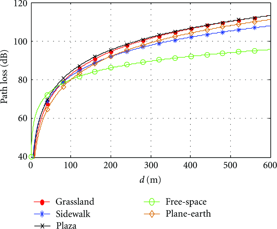
Comparisons between the proposed model and the generic model (
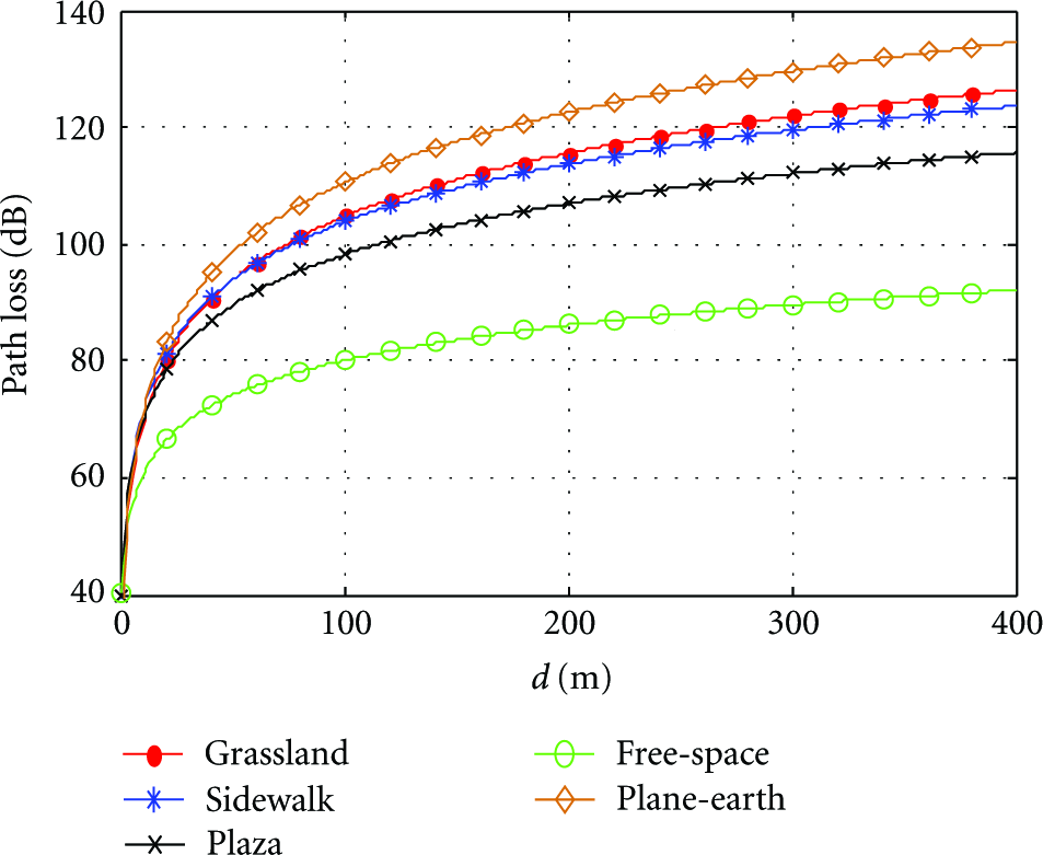
Comparisons between the proposed model and the generic model (
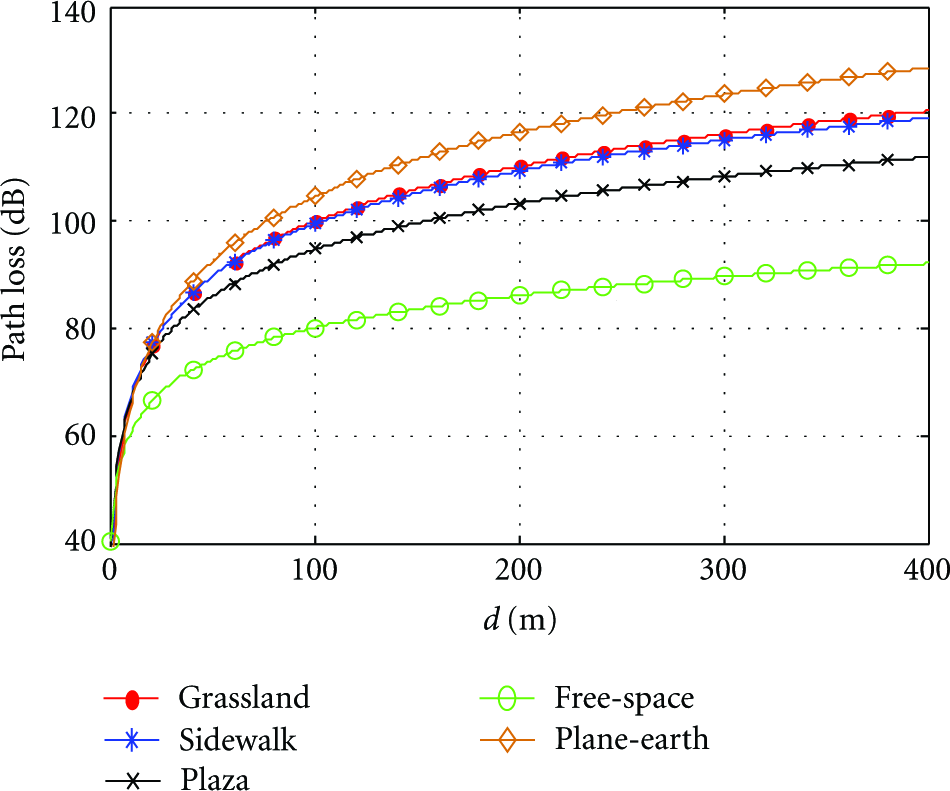
Comparisons between the proposed model and the generic model (
From Figure 6, it is found that the values predicted by the plane-earth model are close to the values predicted by the proposed model, and the difference at 600 m is by 2.1–3.2 dB. This is because the LOS conditions are present in the three sites when both the antenna heights are set to 1 meter, where the two-ray propagation mechanism is dominant. Since the optimization of the plane-earth model is based on the two-ray propagation mechanism [19], its high prediction accuracy is expected. As the transmitting antenna height decreases, the ability of the plane-earth model to predict the path loss becomes poor. As can be seen from Figures 7 and 8, the plane-earth model overestimates the path loss significantly by 8–18.8 dB more than the value predicted by the proposed model at 400 m. This is mainly due to the disappearance of the LOS conditions when the transmitting antenna height is lowered, and other propagation mechanisms are not taken into account by the plane-earth model, such as the forward scattering mechanism mentioned in Section 4.1. On the contrary, the free-space model underestimates the path loss dramatically by 19.8–34.3 dB at 400 m, which further indicates that the near-ground channel is far from a free space.
The unfitness of these two generic models can be further verified by the
5. Conclusions
This paper performs experimental path loss modeling for three near-ground sites at 2.4 GHz frequency. The linear regression based on the measured data indicates that the log-distance-based model is still suitable for path loss modeling in near-ground sites, and the prediction accuracy of the two-slope model is higher than that of the one-slope model. The obtained path loss exponent is less than 2 before the breakpoint and then between 2 and 4, which is in accordance with the results in [17]. The breakpoint distance is mainly determined by the antenna height with slight environmental influences, which is contrary to the conclusions in [3]. For the sidewalk and the grassland sites, an increase of 4.31–5.9 dB in the path loss is observed as the receiving antenna height decreases from 2 to 1 m, which roughly accords with the rule that the path loss increases by 6 dB as the antenna height is halved. However, in cases of much lower antenna height, the path loss increases by 20.1–21.97 dB as the transmitting antenna height decreases from 1 m to 3 cm, suggesting that this rule is not applicable. The proposed model for each site is well matched with the authentic channel environment, which is further verified by the comparisons between the predicted path loss and the measured path loss in far field. Comparisons between the proposed model and the generic models indicate that the near-ground channel (with flat terrain) is far from a free space, and the free-space model will lead to large errors for the path loss prediction. Although the plane-earth model takes the effect of antenna height into consideration, its ability to accurately predict the path loss is still poor. To achieve higher prediction accuracy, the path loss modeling based on the measured data is very necessary. The results presented here can thus be referred for the design and performance simulation of WSN systems in near-ground scenarios.
Footnotes
Acknowledgment
This work was partly supported by the Foundation of National Key Laboratory for Electronic Measurement Technology, China (2011YF003).