Sage Journals: Discover world-class research

Abstract

Wall temperature of an internally finned tube has been computed numerically for different fin number, height, and shape by solving conservation equations of mass, momentum, and energy using Fluent 12.1 for a steady and laminar flow of fluid inside a tube under mixed flow condition. It has been found that there exists an optimum number for fins to keep the pipe wall temperature at a minimum. The fin height has an optimum value beyond which the wall temperature becomes insensitive to fin height. For a horizontal tube, under mixed flow condition, it is seen that the upper surface has higher average temperature than the lower surface. The impact of fin shape on the heat transfer rate shows that wall temperature is least for triangular-shaped fins, compared to rectangular- and T-shaped fins. In addition to the thermal characteristics, the pressure drop caused due to the presence of fins has also been studied.

1. Introduction

Laminar mixed convection and conduction across a heated finned tube has practical implications. Internally finned tubes are commonly used in engineering applications as effective and efficient means to improve convective heat transfer in compact heat exchangers. In the light of recent economic and environmental concerns, researchers are aggressively looking for new methods of heat transfer control both in external-finned and internal-finned heat exchangers.

Internally finned tubes perform differently depending on whether the flow is laminar or turbulent. Laminar flow heat transfer in tubes finds wide engineering applications in many practical fields which include heating or cooling of viscous liquids in the process industries, heating or cooling of oils, heating of circulating fluid in solar collectors, and heat transfer in compact heat exchangers.

For laminar flow and heat transfer, comprehensive experimental and numerical investigations have been performed for variable fluid properties, mixed convection, and fin geometry. Heat transfer augmentation techniques play a vital role here since heat transfer coefficients are generally low for laminar flow in plain tubes. Designing a tubular heat exchanger with fins having different shapes and sizes is one such augmentation technique discussed in this paper.

When an array of fins is used to enhance heat transfer, the prime focus is to optimise geometry of fins which will maximise the heat transfer rate under space and cost constraints. The heat transfer to the fluid flowing through a finned tube by the heat dissipating surfaces can be obtained mainly by using the mechanisms of heat transfer by forced convection.

Extensive work has been carried out by different researchers to analyse heat transfer rate and pressure drop characteristics from tubes having fins of various shapes (rectangular, triangular, T-sectional, and twisted). Experimental investigations have been performed by different researchers to study the friction factor, heat transfer rate, and pressure drop and temperature distribution of tube wall.

Microfins offer effective heat transfer and are more suitable as better heat exchanging medium than twisted tubes. Smit and Meyer [1] performed an experiment to compare three different (microfins, twisted tapes and high fins) heat transfer enhancement methods to that of smooth tubes using the geotropic refrigerant mixture R-22/R-142b. The results corroborated the effectiveness of microfins over twisted tubes.

O’Brien and Sohal [2] investigated experimentally forced convection heat transfer in a narrow rectangular duct fitted with a circular tube and/or a delta-winglet pair. They obtained a comparison of local and average heat transfer distributions for the circular tube with and without winglets and found that at higher Reynolds numbers the enhancement level is close to 50%. Moreover, the combined effect of heat transfer rate and pressure drop depends on the enhancement of baseline-winglet pair. In a study by Chu et al. [3], it has been established that the reduction in the average intersection angle between the velocity vector and the temperature gradient is one of the essential factors influencing heat transfer enhancement. Experimental outcomes in a comparative study with 1-inline, 3-inline, and 7-inline show that the relative performance reduces as the number of inline winglets increases from 1 to 7.

He et al. [4] experimentally evaluated an improvement of 25–55% of heat transfer coefficient and a pressure drop of 90% on air side of a heat exchanger by using a winglet-type vortex generator with attack angle 30°, over $1400 < Re < 3400$ .

Liou et al. [5] showed that the delta wing I and 45°V models give better thermal performance comparing heat transfer enhancement and uniformity and friction loss on 12 configurations of single longitudinal vortex generator in thick boundary layers. Using a modified pressure coefficient, it is found that the mean wall pressure distribution in the wake collapses on to a single curve for several different apex angles of pyramids and angles of attack.

While fins offer solutions to augment heat exchange problems, they also result in pressure drop of flow. Experimental investigations show that the heat transfer characteristics and flow friction are greatly influenced by the fin spacing, size and shape of the fin. Bilir et al. [6] investigated effects of vortex generators on heat transfer and pressure drop characteristics on fin-and-tube heat exchanger with three different types of vortex generators. The cumulative effect of vortex generators offers a better heat exchange solution with moderate drop in pressure. Mohammed and Salman [7] conducted an experiment to study pressure drop and heat transfer characteristics of water flow in a horizontal tube with or without longitudinal fins and found that heat transfer enhancement is 16 times more and friction factor is 4.5 times more of a finned tube than a bare tube having $Re < 4000$ .

Zhu and Li [8] focused on model and simulation of four types of basic fins (plain fin, strip fin, offset fin, perforated fin, and wavy fin) considering fin thickness, thermal entry effect and end effect for $132.3 < Re < 1323$ . They also verified the experimental data with the simulation model. Tatsumi et al. [9] examined experimentally and numerically parallel cut fin array for the purpose of enhancing the fluid mixing and heat transfer and also reducing the pressure loss. They found that the heat transfer coefficient remained almost constant in the plain-fin case but increased in the cut-fin case.

Chiu et al. [10] have done experimental and numerical investigation for analysing conjugate heat transfer in horizontal channels with heated section and the impact on thermal processing techniques. The operational parametric study related to the conjugate heat transfer revealed that the addition of conjugate heat transfer significantly affects the temperature and heat transfer rates at the heated region's surface.

Silva et al. [11] have studied the effect of dimple shape and orientation on the heat transfer coefficient of a vertical fin surface under a laminar flow condition ( $500 < Re < 1000$ ) experimentally as well as numerically. The results revealed that oval dimples with their “long” axis oriented perpendicularto the direction of the flow offered the best thermalimprovement (Nusselts number increased up to 10.6% for the dimpled surface).

Abu-Hijleh [12] numerically analysed cross flow-forced convection heat transfer from a horizontal cylinder with multiple, equally spaced, high-conductivity permeable fins on its outer surface and concluded that permeable fins provided much higher heat transfer rates compared to the more traditional solid fins for a similar cylinder configuration.

Sakalis and Hatzikonstantinou [13] studied numerically the effect of nondimensional fin height (fin height/tube radius) on friction numbers and found that the friction number and Nusselt number are directly related with the fin height and reach critical value at 0.85 and 0.73, respectively.

Lid-driven cavity fluid flow is one of the methods to augment heat transfer and enhance the total quality of thermal system. Sun et al. [14] used finite-volume-based computational method to study the effect of positioning the fin on wall on the heat transfer rates for a forced convection case. The results confirmed that positioning the fin on the right wall while increases the heat transfer on left wall, is opposite on the right and bottom wall.

Park et al. [15] had analysed the effect of heat transfer in a heat sink due to the dimpled surface under laminar airflow. They had considered two different shape (circular and oval) dimples to investigate both numerically as well as experimentally. It was found a 6% heat transfer enhancement relative to a flat plate for Reynolds number range 500 to 1650 on both circular and oval dimples.

Haldar et al. [16] numerically analysed laminar-free convection about a horizontal cylinder with external longitudinal fins of finite thickness and suggested that among the various fin parameters, thickness plays the most influential role in determining the performance of the fins. The optimum number and length of the fins were found as 6 and 0.2 m, respectively, at which the rate of heat transfer is found to be maximum.

Duplain and Baliga [17] had formulated and demonstrated a computational methodology for optimization of fin shapes of steady, laminar, fully developed forced convection in a straight duct of circular cross-section, with air as the fluid and nontwisted, uninterrupted, longitudinal internal-fins made of steel, aluminium, and copper.

A parametric investigation of turbulent flow and heat transfer characteristics of an internally rectangular-finned tube has been done by Liu and Jensen [18]. They concluded that the effects of fin profile, fin number (N), fin width (W_f), and fin height (H) have a significant effect on Nusselt number and friction factor.

The numerical analysis of earlier researchers mostly assumed isothermal fins at the base and constant fluid properties. However, these assumptions greatly influence the pressure drop and heat transfer characteristics. This paper reports the numerical investigation of mixed convection and conduction heat transfer from rectangular fin arrays which are mounted on the inner wall of a horizontal tube. Initially, the investigation is started from matching the present CFD results with the existing analytical results for the case of two dimensional axi-symmetric smooth tubes. Then numerical analysis has been performed to determine the wall temperature distribution and average heat transfer coefficient of rectangular longitudinal fins mounted at the inner periphery of the tube. The flow of air through the tube is considered to be laminar with density taken as the function of temperature according to ideal gas relation, and the wall is subjected to constant heat flux. Then the investigation is carried forward by changing the spacing between the fins, shape, and size to analyse its heat transfer and fluid flow characteristics.

2. Mathematical Modeling

2.1. Mathematical Formulation

The computational investigation is carried out for an internally finned tube of diameter D and length L as shown in Figure 1. Air enters into the tube at one end whereas the other end is exposed to the surrounding atmosphere. Longitudinal fins are placed symmetrically around inner periphery of the tube. The investigation is initiated with the rectangular fins of length L_f, width W_f, and height H_f as shown in Figure 1, and subsequently the cross-sectional area of the fin has been changed to triangular and T shapes. The flow field in the domain would be computed by using three-dimensional, incompressible Navier-Stokes equations (2D axi-symmetric model for simple tube) along with the energy equations. The fluid used in the simulation is air, at temperatures of 300 to 700 K, and is treated to be incompressible (as M = 0.0007), at the inlet face of the tube with an inlet velocity of 0.264 m/s.

Figure 1:

Schematic diagram of computational domain and the boundary condition applied to it.

2.2. Governing Equations

The governing equations for the above analysis can be written as [19].

Continuity equation:

\begin{matrix} \nabla \cdot (ρ \vec{v}) = 0, \end{matrix}

(1)

Momentum equation:

\begin{matrix} \frac{D (ρ U_{i})}{D t} = - \frac{\partial p}{\partial x_{i}} + \frac{\partial}{\partial x_{j}} [μ (\frac{\partial U_{i}}{\partial x_{j}} + \frac{\partial U_{j}}{\partial x_{i}})] - (ρ_{\infty} - ρ) \vec{g}, \end{matrix}

(2)

\begin{matrix} \frac{p}{ρ} = R T . \end{matrix}

(3)

Variable R is the characteristic gas constant and is equal to 0.287 kJ/kg-K.

The density ρ is taken to be a function of temperature according to ideal gas law as per (3), while laminar viscosity μ and thermal conductivity are kept constant. The Boussinesq approximation is not adopted in the model since the variation of ρ with temperature is very high in the range of operating parameters.

Energy equation:

\begin{matrix} \frac{D (ρ T)}{D t} = \frac{\partial}{\partial x_{i}} [\frac{μ}{P r} \frac{\partial T}{\partial x_{i}}] . \end{matrix}

(4)

Conduction equation:

\begin{matrix} \frac{\partial}{\partial x_{i}} (k \frac{\partial T}{\partial x_{i}}) = 0 . \end{matrix}

(5)

2.3. Boundary Conditions

The boundary conditions can be seen from Figure 1. The tube wall and fin are solid and have been given a no-slip boundary condition. Pressure outlet boundary condition has been imposed at the outlet of the tube, and constant heat flux condition is applied on the wall of the tube. The velocity inlet boundary condition has been employed at the inlet face which supplies air into the tube. 2D axi-symmetric model has been used in case of finless tube as in Figure 2.

Figure 2:

Smooth tube 2D axi-symmetric model.

At the pressure outlet boundary, the velocity will be computed from the local pressure field so as to satisfy the continuity, but the scalar variable such as temperature T is computed from the zero gradient condition, Dash [20].

2.4. Computations of Some Important Heat Transfer and Fluid Flow Parameters

The local Nusselt number for the finned heated tube is computed as given in Dogan and Sivrioglu [21]

\begin{matrix} {Nu}_{x} = \frac{h_{x} D_{h}}{k_{air}} . \end{matrix}

(6)

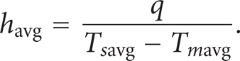
And the local heat transfer coefficient has been computed as given below:

\begin{matrix} h_{x} = \frac{q}{T_{sx} - T_{cx}}, \end{matrix}

(7)

where h_x, D_h, and k_air are the local heat transfer coefficient, hydraulic diameter and thermal conductivity of air, respectively. T_sx and T_cx are the local tube wall temperature and local centreline fluid temperature.

The dimensionless numbers affecting the heat transfer and fluid flow are the Reynolds number:

\begin{matrix} Re = \frac{V_{in} D_{h}}{ν_{air}}, \end{matrix}

(8)

the Grashof number Gr:

\begin{matrix} Gr = \frac{(g β (T_{out} - T_{in}) D_{h}^{3})}{(ν_{air}^{2})}, \end{matrix}

(9)

the Richardson number:

\begin{matrix} Ri = \frac{Gr}{{Re}^{2}} . \end{matrix}

(10)

If $Ri > 1$ , then the flow is dominated by natural convection whereas, for $Ri < 1$ , the flow is dominated by forced convection. This has been discussed in detail in Section 4.4.

The hydraulic diameter of the fin channel is defined as

\begin{matrix} D_{h} = \frac{4 P}{A_{c}}, \end{matrix}

(11)

where A_c is the minimum heat exchanger flow area and P is the wetted perimeter.

However, in case of plane tube without fin, the calculation of mean fluid temperature and the surface temperature has been computed as given in the Incropera and DeWitt [22]:

\begin{matrix} T_{mx} = T_{mi} + \frac{q P}{\dot{m} c_{p}} x, \end{matrix}

(12)

where T_mx is the mean fluid temperature at a particular section along the axial direction of the tube, T_mi is the inlet fluid temperature, q is the constant surface heat flux, P is the surface perimeter which is calculated by $(P = π D)$ , $\dot{m}$ is the mass flow rate of air, C_p is the specific heat of air and is taken as constant value of 1.007 kJ/kg-K, and x is the axial distance.

\begin{matrix} \dot{m} = ρ v A, \end{matrix}

(13)

where ρ is the density of air at inlet of tube.

\begin{matrix} T_{sx} = T_{mx} + \frac{q}{h}, \end{matrix}

(14)

T_sx is the local surface temperature at a particular section.

Now to calculate the local heat transfer coefficient in case of smooth tube, applied constant heat flux at the wall is calculated from the following relation:

\begin{matrix} h_{x} = \frac{q}{T_{sx} - T_{mx}} \end{matrix}

(15)

\begin{matrix} {Nu}_{avg} = \frac{h_{avg} D_{h}}{k_{air}} \end{matrix}

(16)

\begin{matrix} h_{avg} = \frac{q}{T_{s avg} - T_{m avg}} . \end{matrix}

(17)

3. Numerical Solution Procedure

Three-dimensional equations of mass, momentum, and energy have been solved by the algebraic multigrid solver of Fluent 12.1 in an iterative manner by imposing the above boundary conditions. First order upwind scheme (for convective variables) was considered for the momentum equations. After a first-hand converged solution could be obtained, the scheme was changed over to second-order upwind so as to get little better accuracy (wall temperature distribution was changed by only 0.5%). A detailed description of the types, and number of grids used has been discussedseparately in Section 4.

SIMPLE algorithm with a PRESTO scheme for the pressure velocity coupling was used for the pressure correction equation and the cell-face values of pressure could be obtained from simple arithmetic averaging of centroid values. However, it is to be noted as the density becomes a function of temperature then the SIMPLE algorithm for pressure velocity coupling will not work properly because the pressure variation from cell to cell will not be smooth due to the presence of source term in the momentum equation. So in order to obtain the cell-face pressure, new pressure interpolation technique is needed which is available through body force weighted or PRESTO (Pressure Staggered Option) scheme in Fluent.

The body-force-weighted scheme computes the face pressure by assuming that the normal gradient of the difference between pressure and body forces is constant. This works well if the body forces are known a priori in the momentum equations (e.g., buoyancy and axi-symmetric swirl calculations).

The PRESTO (Pressure Staggering Option) scheme uses the discrete continuity balance for a “staggered” control volume about the face to compute the “staggered” (i.e., face) pressure. This procedure is similar in spirit to the staggered-grid schemes used with structured meshes. Note that for triangular, tetrahedral, hybrid, and polyhedral meshes, comparable accuracy is obtained using a similar algorithm. The PRESTO scheme for pressure interpolation is available for all meshes in Fluent.

Under relaxation factors of 0.3 for pressure, 0.6 for momentum and 0.8 for temperature were used for the better convergence of all the variables. Hexahedral cells were used for the entire computational domain. Convergence of the discretized equations was said to have been achieved when the whole field residual for all the variables fell below 10⁻³ for u, v, w, and p, whereas for energy the residual level was kept at 10⁻⁶.

4. Results and Discussion

4.1. Matching with Analytical Solution

We compared the computed surface temperature distribution, axial mean temperature, and surface heat transfer coefficient for a smooth tube with available analytical solution in the standard text of Incropera and DeWitt [22]. Figure 2 shows the schematic diagram of computational domain with the applied boundary condition. In the present analysis, we have considered a tube of length 5 m, diameter 0.07 m, and the flow is considered to be laminar of Re = 1200. The tube wall is subjected to a constant wall heat flux 200 W/m². A comparison for the axial temperature distribution between present CFD method and existing analytical results given by (12) [22] has been shown in Figure 3. It can be seen from the plot that the present CFD results match well with the analytical results. Figure 4 shows the wall temperature distribution for a smooth tube and a comparison between the present CFD results with the existing analytical solution given by (14) [22]. It can be seen from Figure 4 that the wall temperature distribution is almost linear after a tube length around 3 m as the flow is thermally developed fully after this length and the present CFD results for wall temperature distribution matched well with the analytical solution.

Figure 3:

Smooth tube's mean fluid temperature distribution: a comparison between present CFD results with the analytical solution.

Figure 4:

Smooth tube surface's temperature distribution: a comparison between present CFD results with the analytical solution.

Figure 5 shows the surface heat transfer coefficient of smooth tube which has been computed analytically from (15) [22] and subsequently validated with the present CFD method. All the data used for the computation have been shown in the plot itself. Here, the surface heat transfer coefficient of smooth tube computed analytically is matched well with the present CFD results.

Figure 5:

Smooth tube surface's heat transfer coefficient: a comparison between present CFD results with computed analytical solution.

Rate of heat transfer to the air flows inside a finned tube depends upon the fin surface area and internal surface area tubes exposed to the air flows inside it. The heat transfer coefficient varies considerably by varying fin parameters, namely, fin numbers, fin height, and shape of the fins, and at the same time the boundary layer growth affects the heat transfer rate.

4.2. Effect of Cell Number on Surface Temperature Distribution

The numerical investigation is initiated from a grid-independent test as shown in Figure 6. The present numerical analysis is carried out for a 0.07 m diameter tube with a length of 5 m for a laminar flow of Re = 1200 that is subjected to a constant wall heat flux of 200 W/m² and the other parameters can be seen from the plot itself. The number of cells is varied from 80000 to 580000 and the corresponding wall temperature distribution and average wall temperature have been shown in Figure 6. Here, we have conducted a comparison of wall temperature distribution for different number of cells started from 80,000 to 580000. It can be seen from the plot when the number of cells is increased from 80000 to 110000 (around 1.375 times), the average wall temperature increases from 464 K to 468 K (i.e., around 0.8%) but when the cell number is increased further to 150000 (1.36 times), the wall temperature does not vary significantly only 468 K to 469 K (around 0.2%). Then, we adopted the cells in and around the fins so that the cell number is increased from 150000 to 240000 (around 1.6 times). It can be seen from the plot that the wall temperature distribution raises a little when the cell number is increased from 150000 to 240000; whereas the average temperature is increased from 469 K to 473 K (around 0.85%). When the cell number is increased from 240000 to 580000, the average surface temperature does not vary any more, whereas there is hardly any variation of wall temperature distribution. So we performed all the numerical computation when the cell number is around 240000. However, when we change the geometry, we again perform the grid independence test before reporting any results.

Figure 6:

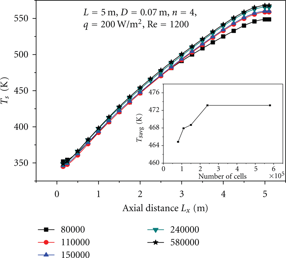
Wall surface temperature distribution as a function of number of cells.

4.3. Effect of the Fin Number on Surface Temperature Distribution

The wall temperature distribution as a function of fin number has been shown in Figure 7. Here, for the present numerical analysis, we have considered a finned tube of length ( $L = 5.1$ m) having 0.1 m inlet section ( $D = 0.07$ m) and 5 m heated section inside which fins are attached internally. Fins are having length (L_f) 5 m, height (H_f) 0.0125 m, and thickness (W_f) 0.008 m. The air flow inside the tube is considered to be laminar having a Reynolds number of 1200 and the tube wall is subjected to a constant heat flux of 200 W/m². The wall temperature distribution for finless tube and tube having different fin number has been shown in Figure 7. It can be seen from the plot that the wall temperature is low for the case of finned tube compared to finless tube suggesting more heat transfer to air flows inside the tube. As the fin number is increased, the average wall temperature is found to be minimum (around 470 K) for a fin number 10 and after that it shoots up to 480 K when the fin number is increased to 12. It clearly indicates that the average heat transfer coefficient is maximum when the number of fins is attached to the internal surface of the tube is 10.

Figure 7:

Tube surface temperature as a function of fin number.

4.4. Effect of Bouncy on Wall Temperature Distribution

The effect of buoyancy on wall temperature can be visualized from Figure 8. The numerical analysis has been conducted with 5.1 m length tube having four numbers of fins attached inside periphery of the tube. The wall of the finned tube is given a constant heat flux of 200 W/m² with Re of 1200. It can be seen from Figure 8 that there is a remarkable difference of the temperature distribution of top wall (corresponding to $θ = 90^{°}$ ) and bottom wall ( $θ = 270^{°}$ ) of the tube. This probably occurs due to the bouncy effect. The dominance of buoyancy effect in the flow depends on the Ri which is given by Gr/Re² and has been discussed in detail for the present case. In the present investigation, we are maintaining Re as 1200 and the Gr we have computed for the present case is 7182781 and we have found $Ri = 4.99$ $(Ri > 1)$ , which clearly indicates the flow is dominated by the buoyancy effect. It is also seen from the figure that the difference of wall temperature distribution is becoming more and more prominent as we proceed in the downstream of flow. So from the present investigation, it can be concluded that due to the effect of the buoyancy, the hot fluid moves to the top wall of the tube which causes higher wall temperature compared to bottom wall.

Figure 8:

Effect of buoyancy on the wall temperature distribution.

4.5. Effect of Fin Height on Temperature Distribution

The wall temperature distribution as a function of fin height has been presented in Figure 9. The numerical analysis has been carried out for different height of the fin while the length and width of the fin is maintained constant. The finned tube wall is maintained a constant heat flux of 200 W/m² and the other operating parameter can be seen from the plot itself. It can be seen from the plot that by increasing the depth of the fin, the wall temperature decreases and reached to minimum for a depth 0.026 m and after that the wall temperature does not fall any more even if we increase fin height. Also we cannot increase the depth beyond 0.03 m because of dimension limitations of the tube. However, it is also seen from the plot that the average Nusselt number continuously increases with fin height suggesting that the heat transfer to the fluid is more due to convection rather than conduction. So, from the present investigation, it can be conclude that the maximum heat transfer occurs for a depth of fin 0.026 m.

Figure 9:

Wall surface temperature distribution and Nusselt number as a function of fin height.

4.6. The Effect of Fin Profile on Surface Temperature Distribution

The shape of the fin profile plays a crucial role on wall temperature distribution which has been shown in Figure 10. For the present numerical analysis three different types of fins have been chosen having cross-sectional area of rectangular-, triangular- and T-shaped where we would be able to keep the volume of the fins constant. The tube wall is subjected to constant heat flux of 200 W/m², and other operating parameter can be seen from the plot. It is evident from the figure the wall temperature is minimum for triangular-shaped fin compared to other shape. It can be also seen from the plot that the average Nusselt number is highest in case of triangular-shaped fin which signifies more heat transfer occurs due to convection in case of triangular-shaped fin compared to other shape. This indicates that the heat transfer is highest in case of triangular fin. It seems that the average heat transfer coefficient is higher for triangular fin compared to other sections.

Figure 10:

Wall surface temperature distribution and Nusselt's number as a function of fin shape.

4.7. Variation of Local Nusselt Number Distribution along the Downstream of Flow

The Nusselt number variation as a function of axial distance of a finned tube has been shown in Figure 11. It can be seen from Figure 11 that the local Nusselt number is initially very high at the inlet of the tube, signifying the dominance of convective heat transfer over conductive transfer and it decreases continuously along the downstream of flow and reaches a minimum value at around 4 m from the entrance of the tube and increases further towards the end of the tube. Due to the growth of thermal boundary layer, the Nusselt number decreases up to a certain distance suggesting the dominance of conduction heat transfer. However, after 4 m, the Nusselt number increases again which signifies the effect of convective heat transfer is becoming more pronounced due to the buoyancy effect. Even with variable thermal conductivity (shown in Figure 12), the Nusselt number variation along the downstream of the finned tube shows that the minimum value exists at a distance of 4 m from the entrance of the tube. Higher value of Nusselt number at the entrance of the finned tube for the case variable thermal conductivity compared to average thermal conductivity shows that conduction heat transfer does not play any significant role at the beginning of the tube. However, towards the end of the tube the variable conductivity Nusselt number is lower compared to average conductivity Nusselt number which signifies the dominance of conductive transfer.

Figure 11:

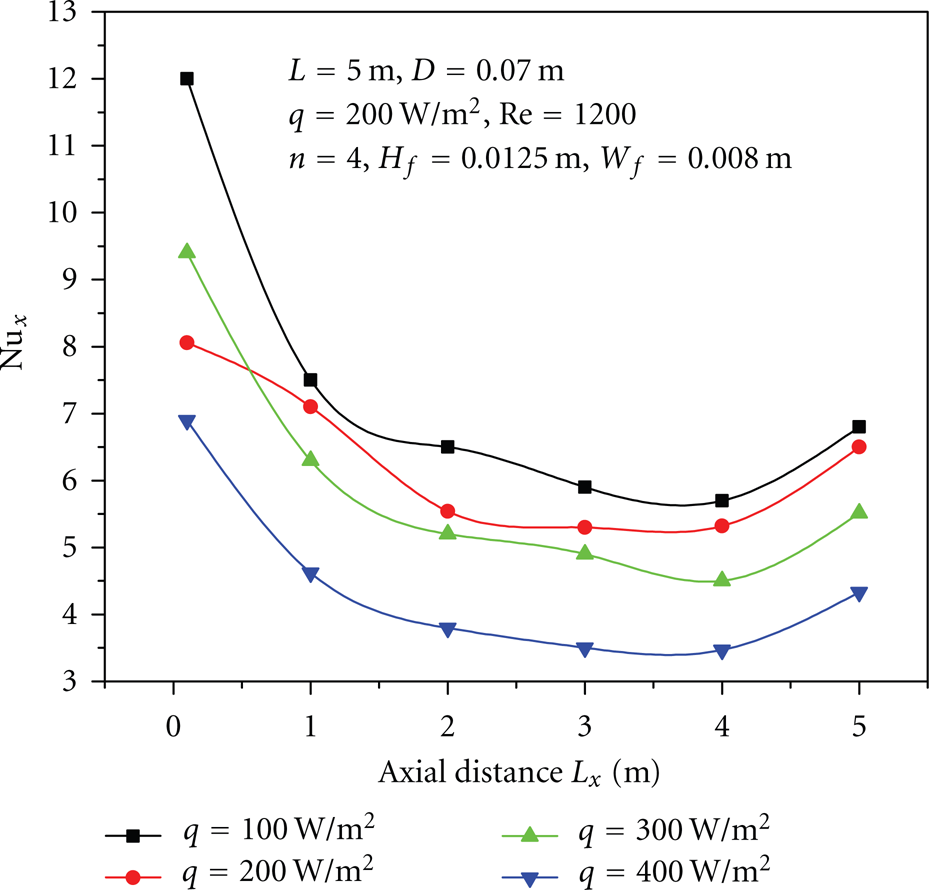
Nusselt's number as a function of axial distance for different heat flux.

Figure 12:

Variation of local Nusselt number as a function of axial distance: a comparison of Nusselt's number for average thermal conductivity and variable thermal conductivity.

4.8. Variation of Pressure Drop along the Downstream of the Flow for Different Fin Number

The axial pressure distribution as shown in Figure 13 varies linearly along the length of the tube. The numerical investigation has been performed for finless tube and also for finned tube having fin number 4, 8, and 12. It can be clearly visualised from the plot for the same Reynolds number as the fin number increases, the pressure drop is also becoming more and more. This signifies as the number of fins increases more and more, pumping power is required to deliver same amount of fluid.

Figure 13:

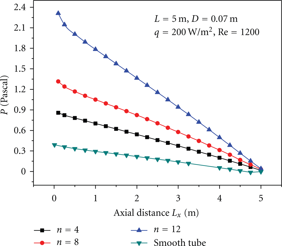
Variation of pressure drop as a function of axial distance for different fin number.

5. Conclusions

The numerical investigation concentrates on wall temperature distribution of an internally finned tube for the case of laminar flow and their validation with existing analytical results of axisymmetry plain tube for axial temperature distribution, surface temperature distribution, and the surface heat transfer coefficient. The following conclusions can be reached from the present investigation.

There exists an optimum fin number for which the heat transfer to the air is maximum and in the present case the optimum number of fin is found to be 10.

There exists an optimum fin height of 0.026 m, where the rate of heat transfer is maximum after which the rate of heat transfer remains unchanged.

For same volume, it is seen that the heat transfer is maximum for triangular-shaped fin as compared to rectangular- and T-shaped fin.

It is also evident from the present investigation the heat transfer is more from the bottom wall ( $θ = 270^{°}$ ) compared to top wall ( $θ = 90^{°}$ ) due to buoyancy effect.

Heat is conducted to the air at the entrance, and after a certain distance, the convective transfer becomes more predominant.

Footnotes

Nomenclature

Greek Symbols

Subscripts

References

Smit

F. J.

and Meyer

J. P.

, “R-22 and zeotropic R-22/R-142b mixture condensation in microfin, high-fin, and twisted tape insert tubes,” Journal of Heat Transfer, vol. 124, no. 5, pp. 912–921, 2002.

O'Brien

J. E.

and Sohal

M. S.

, “Heat transfer enchancement for finned-tube heat exchangers with winglets,” Journal of Heat Transfer, vol. 127, no. 2, pp. 171–178, 2005.

Chu

Y. L.

, and Tao

W. Q.

, “Three-dimensional numerical study of flow and heat transfer enhancement using vortex generators in fin-and-tube heat exchangers,” Journal of Heat Transfer, vol. 131, no. 9, Article ID 091903, 9 pages, 2009.

Liu

, and Jacobi

A. M.

, “Air-side heat-transfer enhancement by a new winglet-type vortex generator array in a plainfin round-tube heat exchanger,” Journal of Heat Transfer, vol. 132, no. 7, Article ID 071801, 9 pages, 2010.

Liou

T. M.

Chen

C. C.

, and Tsai

T. W.

, “Heat transfer and fluid flow in a square duct with 12 different shaped vortex generators,” Journal of Heat Transfer, vol. 122, no. 2, pp. 327–335, 2000.

Bilir

Ozerdem

Erek

, and Ilken

, “Heat transfer and pressure drop characteristics of fin-tube heat exchangers with different types of vortex generator configurations,” Journal of Enhanced Heat Transfer, vol. 17, no. 3, pp. 243–256, 2010.

Mohammed

H. A.

and Salman

Y. K.

, “Free and forced convection heat transfer in the thermal entry region for laminar flow inside a circular cylinder horizontally oriented,” Energy Conversion and Management, vol. 48, no. 7, pp. 2185–2195, 2007.

Zhu

and Li

, “Three-dimensional numerical simulation on the laminar flow and heat transfer in four basic fins of platefin heat exchangers,” Journal of Heat Transfer, vol. 130, no. 11, Article ID 111801, 8 pages, 2008.

Tatsumi

Yamaguchi

Nishino

, and Nakabe

, “Flow and heat transfer characteristics of a channel with cut fins,” Journal of Enhanced Heat Transfer, vol. 17, no. 2, pp. 153–168, 2010.

10.

Chiu

W. K. S.

Richards

C. J.

, and Jaluria

, “Experimental and numerical study of conjugate heat transfer in a horizontal channel heated from below,” Journal of Heat Transfer, vol. 123, no. 4, pp. 688–697, 2001.

11.

Silva

Park

Marotta

, and Fletcher

, “Optimization of fin performance in a laminar channel flow through dimpled surfaces,” Journal of Heat Transfer, vol. 131, no. 2, Article ID 021702, 9 pages, 2009.

12.

Abu-Hijleh

B. A. K.

, “Natural convection heat transfer from a cylinder with high conductivity permeable fins,” Journal of Heat Transfer, vol. 125, no. 2, pp. 282–288, 2003.

13.

Sakalis

V. D.

and Hatzikonstantinou

P. M.

, “Laminar heat transfer in the entrance region of internally finned square ducts,” Journal of Heat Transfer, vol. 123, no. 6, pp. 1030–1034, 2001.

14.

Sun

Oztop

H. F.

Wang

, and Wei

, “Control of mixed convection in lid-driven enclosures using conductive triangular fins,” International Journal of Heat and Mass Transfer, vol. 54, no. 4, pp. 894–909, 2011.

15.

Park

Silvas

Marotta

, and Fletcher

, “Study of laminar forced convection heat transfer for dimpled heat sinks,” Journal of Thermophysics and Heat Transfer, vol. 22, no. 2, pp. 262–270, 2008.

16.

Haldar

S. C.

Kochhar

G. S.

Manohar

, and Sahoo

R. K.

, “Numerical study of laminar free convection about a horizontal cylinder with longitudinal fins of finite thickness,” International Journal of Thermal Sciences, vol. 46, no. 7, pp. 692–698, 2007.

17.

Duplain

and Baliga

B. R.

, “Computational optimization of the thermal performance of internally finned ducts,” International Journal of Heat and Mass Transfer, vol. 52, no. 17–18, pp. 3929–3942, 2009.

18.

Liu

and Jensen

M. K.

, “Geometry effects on turbulent flow and heat transfer in internally finned tubes,” Journal of Heat Transfer, vol. 123, no. 6, pp. 1035–1044, 2001.

19.

Mishra

D. P.

and Dash

S. K.

, “Maximum air suction into a louvered funnel through optimum design,” Journal of Ship Research, vol. 56, no. 1, pp. 1–11, 2012.

20.

Dash