Sage Journals: Discover world-class research

Abstract

This paper considers the complexity of the Minimum Unit-Disk Cover (MUDC) problem. This problem has applications in extending the sensor network lifetime by selecting minimum number of nodes to cover each location in a geometric connected region of interest and putting the remaining nodes in power saving mode. MUDC is a restricted version of the well-studied Minimum Set Cover (MSC) problem where the sensing region of each node is a unit-disk and the monitored region is geometric connected, a well-adopted network model in many works of the literature. We first present the formal proof of its NP-completeness. Then we illustrate several related optimum problems under various coverage constraints and show their hardness results as a corollary. Furthermore, we propose an efficient algorithm for reducing MUDC to MSC which has many well-known algorithms for approximated solutions. Finally, we present a decentralized scalable algorithm with a guaranteed performance and a constant approximation factor algorithm if the maximum node density is fixed.

1. Introduction

The research in wireless ad hoc networks has rapidly grown in recent years due to their applications in civil and military domains. Combined with recent developments in micro-electro-mechanical systems and low-cost mass production, various small and low-power devices that integrate sensors with limited on-board processing and wireless communication capabilities begin to emerge. Hence, wireless networks with large numbers of sensors become possible and open up potential of many new applications, such as environment monitoring and surveillance [1].

With the available technology, the sensors are usually battery powered. Due to size and cost constraints, the energy available at each sensor is limited. Therefore, one of the important design considerations in sensor networks is to minimize energy consumption and prolong network lifetime. There is a significant amount of the literature addressing the issue of efficient energy management in generic wireless ad hoc networks from various perspectives, such as medium access control [2, 3], routing [4, 5], broadcasting [6, 7], multicasting [8, 9], and topology control [10, 11]. Of course, similar approaches have been also considered in wireless sensor networks [12–15].

An alternative approach commonly adopted in sensor networks is based on scheduling sensor activity so that some nodes may enter the power saving mode while the remaining active nodes can still provide continuous service [14, 16]. For instance, if all the sensor nodes simultaneously operate in active mode, an excessive amount of energy is wasted and the data collected is highly correlated and redundant. In addition, multiple packet collisions may occur when all the sensors in a certain region try to transmit as a result of a triggering event. Several research results [3, 16] illustrate that a mode of operation alternating active and inactive battery states has a significant reduced energy consumption.

However, such scheduling schemes may face new constraints about sensing coverage introduced by their distributed sensing applications [17]. For example, surveillance applications may require each location of monitored regions to be covered by at least one sensor, while many stronger environmental monitoring, such as military applications, require multiple sensors for fault-tolerant purpose. Besides, triangulation positioning-based tracking applications [18, 19] may require at least three sensors at any locations. Data sampling applications may require a given percentage of monitored regions to be covered.

Therefore, this paper considers the scheduling approach that extends the network lifetime by minimizing the number of active nodes while maintaining coverage constraints. As mentioned earlier, the advantage of this approach is that less packet collisions may occur since less spatially close sensors try to transmit highly correlated and redundant information as a result of a triggering event. Hence, the lifetime of each sensor cover may be extended.

We model a sensor network as a 2D geometric connected region monitored by a set of deployed sensor nodes with unit-disk sensing regions, a realistic assumption that is well adopted in many network models. The coverage constraint is that each location of the 2D region is covered by at least one active node. Note that optimum sensor cover problems may be solved by partitioning monitored regions into disjoint sectors [20, 21]. Here a sector is a maximum region covered by the same set of nodes. Hence the minimum sensor cover problem is transformed to the Minimum Set Cover (MSC) problem which is NP-complete [22] and has been studied extensively in the literature [23–26]. However, with the additional unit-disk sensing region and geometric connected monitored region restrictions, the problem considered here is only a restricted version of MSC, and, to the best of our knowledge, its complexity is still unknown. (That is, it is not trivial to transform each instance of MSC to an instance in the minimum sensor cover problem with unit-disk sensing regions over a connected monitored region in polynomial time.) Thus, we will answer this fundamental question and present the formal proof of its NP-completeness. Furthermore, we illustrate several related optimum problems under different coverage constraints and show their hardness results as a corollary.

Next, we propose the arc sampling algorithm which may effectively and efficiently reduce MUDC to MSC. Consequently, many well-known algorithms can be applied to find approximated solutions. In addition, we present a decentralized scalable algorithm with a guaranteed performance, and a constant approximation factor algorithm if the maximum node density is fixed. Finally, we illustrate simulation results to evaluate the proposed algorithms.

2. Related Work

2.1. Coverage Problems

Meguerdichian et al. [17] defined the coverage problems from several different application domains including deterministic, statistical, worst, and best cases. They also presented optimum polynomial time algorithms to evaluate paths that are the best and least monitored in the sensor network. The work in [27] further defined the exposure problem as measure of how well an object can be observed by the sensor network while it moves along an arbitrary path with an arbitrary velocity. A localized exposure-based coverage algorithm was proposed in [28] for finding the minimal exposure path between two points.

Furthermore, Gui and Mohapatra [29] considered the object tracking applications in which networks operate between surveillance state and tracking state. During surveillance state, they devised a set of metrics for quality of surveillance for detecting moving objects and quantify the trade-off between power conservation and quality. They also proposed an algorithm for each node to determine when to wake up or sleep during the tracking stage.

Tian and Georganas [30] developed a coverage-preserving scheduling scheme to reduce energy consumption by turning off some redundant nodes based on some eligibility rules. Carbunar et al. [31] proposed distributed algorithms for detecting and eliminating redundancy in a sensor network while preserving the network's coverage via Voronoi diagrams, even in cases of sensor failures or insertion of new sensors.

Huang and Tseng [32] considered the k-coverage problem to determine whether every point in the monitored region is covered by at least k nodes. They reduced this problem to the perimeter-coverage problem which determines the coverage degree of the perimeter of each node's sensing region and presented polynomial-time algorithms in the number of nodes.

In addition to coverage, connectivity also needs to be assured to make sensor networks successfully. It has been shown in [33] that if the communication range of sensors is at least twice as large as their sensing range, then full coverage of a convex region implies connectivity. Wang et al. [34] presented a Coverage Configuration Protocol (CCP) that allows the network to self-configure dynamically to achieve guaranteed degrees of coverage and connectivity.

2.2. Minimum Sensor Cover Problems

In [21], Funke et al. proposed the greedy sector cover algorithm which selects a node that covers the maximum number of uncovered sectors at each iteration step. That is, the problem is reduced to MSC and solved by the greedy algorithm. They proved that the well-known approximation factor $O (\log m)$ remains tight in this restricted version. Here m is the maximum number of sectors covered by a single node. To obtain better approximation factors, they also presented a grid placement algorithm and a distributed dominating cover algorithm. These two algorithms have constant approximation factors, but cannot guarantee the full coverage.

Gupta et al. [35] designed an $O (\log | N |)$ centralized approximation algorithms with the connectivity constraint. Here $| N |$ is the number of sensor nodes. In their definition of the sensor cover problem, the sensing region can take any convex shape. They also mentioned that such a problem is NP-hard as the less general problem of covering discrete points using line segments is known to be NP-hard [36]. On the other hand, the sensing region considered in this paper is restricted to a unit-disk, which is well adopted in many network models. We will prove such a problem remains NP-complete even with the unit-disk restriction. They also proposed a distributed algorithm based on node priorities, but did not provide any guarantee on the solution size.

2.3. Related Optimum Problems

Fowler et al. [37] proved the $N P$ -completeness of the Box Cover problem which aims at finding the minimum number of identical rectangles to cover a set of given points. Similarly, Megiddo and Supowit [38] considered the Circle Covering problem which is equivalent to the Geometric Disc Covering problem, that is, to find the minimum number of identical disks to cover a set of given points. There are two fundamental differences between MUDC and these two problems. In these two problems, the covered object is a set of discrete points but not a connected region. Hence, in the proofs of the NP-completeness, we have less flexibility in the connected case than in the discrete cases, since we need to ensure the monitored region is connected while constructing a problem instance. Furthermore, the two problems have the flexibility to determine the “good” locations of covering objects (rectangles or disks), which could be anywhere on the plane. On the other hand, in MUDC, the locations of disks are pre-deployed.

Marathe et al. [39] considered several basic optimization problems for unit-disk graphs with hierarchical structures. They presented a general technique to prove the hardness results of several problems. The hardness of these problems, including Box Cover and Circle Covering, was proved via satisfiability problems. The reduction strategy was to use some geometric structures to represent variables. Each clause is represented by a special structure that “glues” the corresponding structures of the variables in the clause.

There are several polynomial approximation algorithms [40–42] for the Geometric Disc Covering problem. Franceschetti et al. pointed out in [43] that the number of possible disk positions can be bounded if any disk that covers at least two points has two of these points on its border. Hence, by performing a search on a subset of the possible disk positions, the running time of these algorithms becomes polynomial and the solution sizes are guaranteed. They also gave a detailed comparison of these algorithms in [44].

3. Preliminaries

In this section, we define the Minimum Unit-Disk Cover (MUDC) problem that aims at finding the least number of nodes with unit-disk sensing regions to fully cover a designated connected region. We prove this problem is intractable; that is, it belongs to the NP-complete class.

Definition 1.

Consider a two-dimensional Euclidean metric space 𝔼, the unit-disk sensing region of a given node $n \in 𝔼$ is defined as $disk (n) = {x \in 𝔼 | d (x, n) \leq 1}$ . (In the context of discussing MUDC, we represent a node by its geometric location without any confusion.) Here $d (x, n)$ is the distance in Euclidean metric between x and n. Furthermore, the unit-disk sensing region of a set U of nodes is defined as $disk (U) = ⋃_{n \in U} disk (n)$ .

Definition 2.

A two-dimensional finite region A is said to be unit-disk covered by a set U of nodes in a two-dimensional Euclidean metric space if $A \subseteq disk (U)$ . Furthermore, U is called a unit-disk cover (UDC) of A.

The objective is to find the minimum unit-disk cover (MUDC) of A. Note that the optimum problems discussed in this paper could be solved by their associated decision problems in polynomial time. Therefore, we discuss the decision version of MUDC instead, and it can be formally stated in the following.

Problem 3 (MUDC).

Given a set N of nodes in a two-dimensional Euclidean metric space 𝔼, a two-dimensional geometric connected finite region $A \subset 𝔼$ , and a positive integer K, determine whether there is a subset $U \subseteq N$ with $| U | \leq K$ such that $A \subseteq disk (U)$ . Here $| U |$ is the cardinality of U.

For simplicity's sake, the geometry of an MUDC problem, that is, the region A and the set N of nodes, is denoted as $(A, N)$ .

Thus, we will prove the following theorem.

Theorem 4.

MUDC is NP-complete.

The NP-completeness of MUDC will be proved by reduction from the Planar 3-SAT problem, which is known to be NP-complete [45].

Problem 5 (Planar 3-SAT, P3SAT).

Given a set of variables $V = {v_{1}, v_{2}, \dots, v_{η^{'}}}$ and a set of clauses $C = {c_{1}, c_{2}, \dots, c_{η}}$ over V such that each $c \in C$ has $2 \leq | c | \leq 3$ (denoted as a boolean formula B) determine whether there is an assignment for the variables so that all clauses are satisfied. (In Lichtenstein's NP-completeness proof of P3SAT [45], an instance of 3SAT is transformed to an instance of P3SAT with $| c |$ being 2 or 3. Thus, the restriction, $2 \leq | c | \leq 3$ , does not change the complexity of the problem. This restriction is required to prove Lemma 17.) Furthermore, the bipartite graph $G_{B} = {V \cup C, E}$ (in this NP-completeness proof of MUDC, $G_{B}$ will be used to construct an equivalent MUDC problem for B) is planar, where $E = {(v_{i}, c_{j}) | v_{i} \in c_{j} or \overset{̅}{v_{i}} \in c_{j}}$ . (We remove the edges ${(v_{i}, v_{i + 1}) | 1 \leq i < m^{'}} \cup {(v_{m^{'}}, v_{1})}$ without any changes in the difficulty of the problem [46].)

That is, let B be a boolean formula in P3SAT with η clauses and $η^{'}$ variables. We wish to construct an equivalent MUDC problem with the geometry MUDC $(B) = (A_{B}, N_{B})$ where $A_{B}$ and $N_{B}$ are the region and the set of nodes transformed from $G_{B}$ , respectively.

Inspired by Lichtenstein's NP-completeness proof of the Geometric Connected Dominating Set problem [45], MUDC $(B) = (A_{B}, N_{B})$ is constructed via structures. Each structure S is a geometry containing a polygon A and a set of nodes N and denoted as $S = (A, N)$ . Variables, clauses, and edges of $G_{B}$ are represented by various structures. Hence, MUDC $(B)$ is constructed from $G_{B}$ by replacing variables, clauses, and edges with their corresponding structures.

Each structure $S = (A, N)$ is constructed in such a way that N can be partitioned into two disjoint subsets of equal size, denoted as $N^{+}$ and $N^{-}$ , and the MUDC of A, except the ones representing clauses, is either $N^{+}$ or $N^{-}$ . Thus, a variable is assigned true corresponding to that $N^{+}$ is the MUDC of A; false corresponds to $N^{-}$ . For convenience throughout this paper, we assign each node a polarity. The node n has positive polarity if $n \in N^{+}$ or negative polarity if $n \in N^{-}$ . The property of structures mentioned above can be formally defined in the following.

Definition 6.

One calls a structure $S = (A, N)$ well aligned if $A \subseteq disk (N^{+})$ and $A \subseteq disk (N^{-})$ .

Definition 7.

For a structure $S = (A, N)$ and $N^{'} \subseteq N$ , we call S partially well behaved on $N^{'}$ , if the following preconditions hold:

(i)

$| N^{' +} | = | N^{' -} | = | N^{'} | / 2$

(ii)

if $U \subseteq N$ is a UDC of A, $| U \cap N^{'} | \geq | N^{'} | / 2$

(iii)

if $U \subseteq N$ is an MUDC of A, $U \cap N^{'} = N^{' +}$ or $U \cap N^{'} = N^{' -}$ . (For a given set of nodes N, we denote the set of nodes with the same polarity as N with superscripts + or − throughout this paper. i.e., $N^{+} = {n \in N | n has positive polarity}$ and $N^{-} = {n \in N | n has negative polarity}$ .)

Furthermore, we call S well behaved if S is partially well behaved on N.

Note that, from the above definition, if $S = (A, N)$ is well behaved and $U \subseteq N$ is an MUDC of A, then $| U | = | N | / 2$ and U only contains the nodes with the same polarity.

The NP-completeness proof of MUDC will proceed as follows. (1)

Describe structures representing variables, edges, and clauses. These structures have the properties defined in Definitions 6 and 7.

(2)

Describe how the above structures may be connected together to represent $G_{B}$ while preserving the properties defined in Definitions 6 and 7. Here the resulting composite structure is MUDC $(B) = (A_{B}, N_{B})$ .

(3)

We claim that B is satisfiable if and only if $A_{B}$ can be covered by half the nodes of $N_{B}$ . In the proof of the claim, the properties defined in Definitions 6 and 7 will be used in the forward direction and the backward direction respectively.

4. NP-Completeness Proof of MUDC

We first prove that $M U D C$ belongs to the $N P$ class. This could be done since a nondeterministic algorithm needs only guess a set of nodes, U, and verify whether $A \subseteq disk (U)$ . Besides, as stated in [32], this verification could be done in $O ({| U |}^{2} \log | U |)$ .

We continue the proof by reduction from the Planar 3-SAT problem. Let B be a boolean formula in P3SAT with η clauses and $η^{'}$ variables. We wish to construct an equivalent MUDC problem with the geometry MUDC $(B) = (A_{B}, N_{B})$ transformed from the bipartite graph $G_{B}$ .

4.1. Structures

We encode each variable by the structure, denoted as $S_{v} = (A_{v}, N_{v})$ , shown in Figure 1. $A_{v}$ represents the shaded region which is a $d_{v} \times 1$ rectangle. $N_{v}$ represents the set of the $2 (d_{v} + 1)$ nodes which are positioned accordingly and used to cover $A_{v}$ . Each node has a either positive or negative polarity and is represented by a square or triangle, respectively, in the figure. The $d_{v}$ may be long enough to prevent unwanted interactions between nearby edge structures.

Figure 1

The structure representing a variable.

Next, we may encode an edge by a strip-like structure, denoted as $S_{e} = (A_{e}, N_{e})$ , which may extend horizontally and vertically. Figure 2 illustrates an example. The shaded region, denoted as $A_{e}$ , is composed of rectangles. $N_{e}$ represents the set of the positive and negative polar nodes which are positioned accordingly and used to cover $A_{e}$ .

Figure 2

The structure representing an edge.

It is not hard to prove the structures $S_{v}$ and $S_{e}$ satisfy the following lemma.

Lemma 8.

The structures $S_{v} = (A_{v}, N_{v})$ shown in Figure 1 and $S_{e} = (A_{e}, N_{e})$ shown in Figure 2 are well aligned and well behaved.

Proof.

The lemma may be proved by induction. For the sake of brevity, the complete proof is given in Appendix A.

Each clause c may be represented by a structure, called an n -way connector and denoted as $S_{c} = (A_{c}, N_{c} 〈 𝒫, H 〉)$ . Here $n = | c |$ and could be the value of 2 and 3. Figure 3 illustrates the possible realization of n-way connectors. $A_{c}$ represents the shaded polygon that will be covered by the set of the nodes, $N_{c}$ . The geometries of $A_{c}$ and relative positions of nodes of $N_{c}$ are shown in Figures 3 and 4 and Tables 1 and 2.

Table 1

The geometry of the 2-way connector shown in Figure 3(a).

$N_{c}$		$A_{c}$
Node	Position	Vertex	Position

$n_{1}$	(0,0)	$v_{1}$	(0,0)
$n_{2}$	(1,0)	$v_{2}$	(1,0)
$n_{3}$	(1,1)	$v_{3}$	(1,1)
$n_{4}$	(1,2)	$v_{4}$	$(\frac{1}{2}, 1)$
$n_{5}$	(1,3)	$v_{5}$	(1,2)
$n_{6}$	(0,3)	$v_{6}$	(1,3)
$n_{7}$	(0,2)	$v_{7}$	(0,3)
$n_{8}$	(0,1)

Table 2

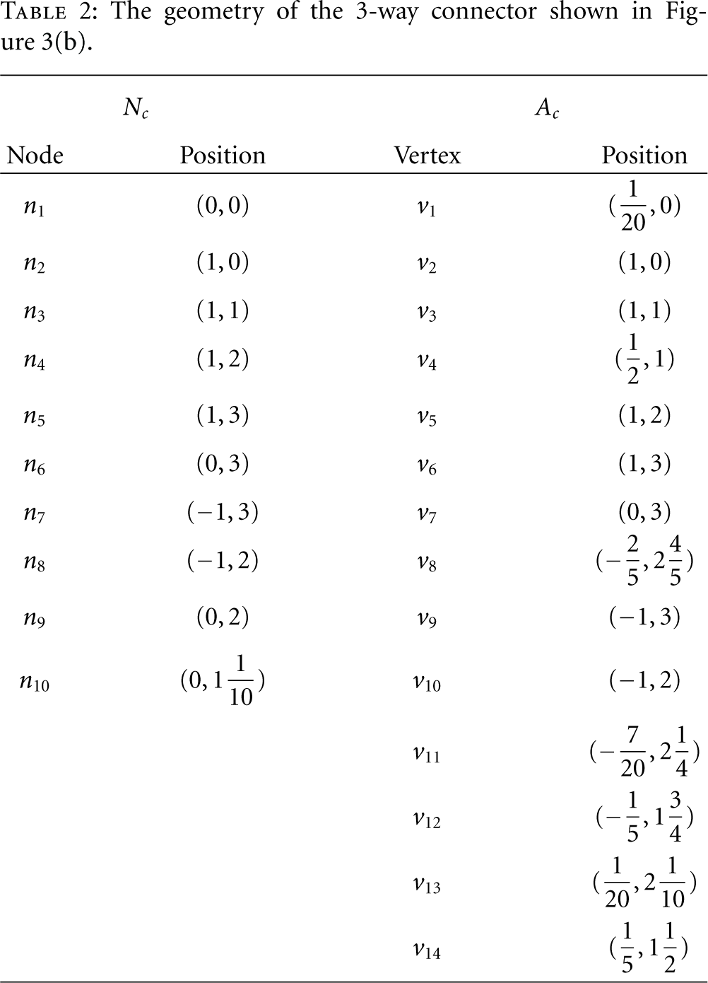
The geometry of the 3-way connector shown in Figure 3(b).

$N_{c}$		$A_{c}$
Node	Position	Vertex	Position

$n_{1}$	(0,0)	$v_{1}$	$(\frac{1}{20}, 0)$
$n_{2}$	(1,0)	$v_{2}$	(1,0)
$n_{3}$	(1,1)	$v_{3}$	(1,1)
$n_{4}$	(1,2)	$v_{4}$	$(\frac{1}{2}, 1)$
$n_{5}$	(1,3)	$v_{5}$	(1,2)
$n_{6}$	(0,3)	$v_{6}$	(1,3)
$n_{7}$	$(- 1,3)$	$v_{7}$	(0,3)
$n_{8}$	$(- 1,2)$	$v_{8}$	$(- \frac{2}{5}, 2 \frac{4}{5})$
$n_{9}$	(0,2)	$v_{9}$	$(- 1,3)$
$n_{10}$	$(0,1 \frac{1}{10})$	$v_{10}$	$(- 1,2)$
		$v_{11}$	$(- \frac{7}{20}, 2 \frac{1}{4})$
		$v_{12}$	$(- \frac{1}{5}, 1 \frac{3}{4})$
		$v_{13}$	$(\frac{1}{20}, 2 \frac{1}{10})$
		$v_{14}$	$(\frac{1}{5}, 1 \frac{1}{2})$

Figure 3

The structures representing clauses.

Figure 4

The labels of $A_{c}$ .

Furthermore, $N_{c}$ is divided into n disjoint partitions $P_{i} \subseteq N_{c}$ with $1 \leq i \leq n$ and we denote $𝒫 = {P_{1}, P_{2}, \dots, P_{n}}$ . As shown in Figure 3, each node is labeled as an alphabet and a numeral. The nodes with the same numeral belong to the same partition. The alphabets represent the relative polarity of nodes within the same partition. For example, in Figure 3(b), the nodes labeled as C2 and D2 belong to $P_{2}$ . The two nodes labeled as C2 have the same polarity and have the opposite polarity with the two nodes labeled as D2.

Each partition $P_{i}$ has a header node $h_{i} \in P_{i}$ which is indicated as a dark circle in Figure 3. We can define the polarity of the partition $P_{i}$ as the polarity of its header node $h_{i}$ . The set of header nodes is denoted as H. Each partition corresponds to a variable of a clause. What n-way connector should represent a clause depends on how the clause is formed from variables. For example, if c is composed of two positive literals and one negative literal, then it should be represented by a 3-way connector that has two positive partitions and one negative partition as shown in Figure 7. As described later, an edge and its ends in $G_{B}$ will be transformed by connecting a variable structure to a partition of an n-way connector via an edge structure. Thus, a partition may be viewed as “extended territory” of a variable. (The definition of territory is given in Definition 16. Again, the key point to transform $G_{B}$ to MUDC $(B)$ is to preserve the properties defined in Definitions 6 and 7 for territories.)

The main reason why an n-way connector is constructed in this way is the following lemma.

Lemma 9.

Each n-way connector, $S_{c} = (A_{c}, N_{c} 〈 𝒫, H 〉)$ , of Figure 3 has the following properties. (i)

$For all P_{i} \in 𝒫$ , $S_{c}$ is partially well behaved on $P_{i}$ . (For an MUDC of $A_{c}$ , the active nodes of each partition have the same polarity. Thus, a variable of c can be assigned true or false based on the polarity of the active nodes in its corresponding partition. Here, in the context of discussing a given UDC, we call a node active if it is in the UDC.)

(ii)

If $U \subseteq N_{c}$ is a UDC of $A_{c}$ , then $H \cap U \neq \emptyset$ . (At least one header node must be active for covering $A_{c}$ .)

(iii)

$A_{c} \subseteq disk (⋃_{1 \leq i \leq n} P_{i}^{p_{i}})$ , if $H \cap ⋃_{1 \leq i \leq n} P_{i}^{p_{i}} \neq \emptyset$ . Here $P_{i}^{p_{i}} \subset P_{i}$ contains either all positive polar nodes ( $p_{i} = +$ ) or all negative polar nodes ( $p_{i} = -$ ). That is, $P_{i}^{p_{i}} = P_{i}^{+} or P_{i}^{-}$ . (In other words, if the active nodes of each partition have the same polarity and one of them is a header node, then $A_{c}$ is covered.)

Proof.

The idea is to examine each possible case of partition $P_{i}$ and ensure $A_{c}$ will not be covered if, for each $P_{i}$ , less than $| P_{i} | / 2$ nodes are active or if exactly $| P_{i} | / 2$ nodes but not having the same polarity are active. Furthermore, we need to examine whether $A_{c}$ will be covered if none of header nodes is active. The complete proof is given in Appendix B.

Note that, from Lemma 9(ii), at least one header node must be active for covering $A_{c}$ . Thus, together with Lemma 9(i), an MUDC of $A_{c}$ will allow each variable of a clause to be assigned true or false, based on the polarity of active nodes in its corresponding partition, for the clause being satisfied.

4.2. Composite Structures

Next, we illustrate how structures may be connected together to form a complex structure. As shown in Figure 5, two structures, $S_{1} = (A_{1}, N_{1})$ and $S_{2} = (A_{2}, N_{2})$ , are connected via several $1 \times 1$ squares called connection patches. Each connection patch has two nodes from each structure, for example, $n_{i}, n_{i + 1} \in N_{1}$ and $n_{j}, n_{j + 1} \in N_{2}$ , located at its vertices. (This is formally defined as precondition 25(i). For convenience sake, we use precondition 25(i) for referring to precondition (i) of Definition 25, and will use this labeling throughout this paper.) Besides, the nodes on the same edge of each connection patch have opposite polarities. (This is formally defined as preconditions 25(ii) and 26(ii).) For the sake of brevity, the formal definitions are given in Appendix C. We call the set $N_{p} = {n_{i}, n_{i + 1}}$ a port of $S_{1}$ , and a port is a connected port if there is a connection patch attaching to it. Besides, the nodes from different structures but on the same edge of a connection patch are each other's connection counterpart, for example, $n_{i}$ and $n_{j}$ . Obviously, it is easy to derive the following lemma.

Figure 5

Connection patches for connecting two structures.

Lemma 10.

A connection patch can be unit-disk covered by the same polar nodes located at its vertices, for example, ${n_{i}, n_{j + 1}}$ or ${n_{i + 1}, n_{j}}$ in Figure 5.

In this $N P$ -completeness proof, in order to preserve the partially well-behaved property, we require two structures to be in such a way, that is, least interactively connected, that (1)

at least one node from each connected port is active, (this is formally defined as precondition 27(i));

(2)

nonconnected port nodes do not cover any point, except the vertices, of the connection patches (this is formally defined as precondition 27(ii) which states whether a connection patch can be fully covered only depends on its connected port);

(3)

nonconnected port nodes of one structure do not cover any region of the other structure, (this is formally defined as precondition 28(i));

(4)

the connected ports of one structure cannot cover any point, except their connection counterparts, of the other structure (this is formally defined as precondition 28(ii));

The formal definitions about the least interactive connection are also given in Appendix C.

A variable structure can use any two nearby nodes on the side of border as a port, for example, ${n_{i}, n_{i + 1}}$ shown in Figure 1. An edge structure uses its endpoints as ports, indicated by the arrows in Figure 2. For an n-way connector, each partition $P_{i}$ contains a port indicated by the arrows in Figure 3. The fact that it is possible to make the above structures least interactively connected via the ports described is proved in Appendix D.

We can define the composite structure in the following definition and derive several lemmas about the least interactive connection. For the sake of brevity, the complete proofs of these lemmas are given in Appendix E.

Definition 11.

The structures $S_{1} = (A_{1}, N_{1})$ and $S_{2} = (A_{2}, N_{2})$ are least interactively connected via the connection patches $A_{c p, 1}, A_{c p, 2}, \dots, A_{c p, T}$ . One calls $S = (A_{1} \cup A_{2} \cup ⋃_{1 \leq t \leq T} A_{c p, t}, N_{1} \cup N_{2})$ the composite structure of $S_{1}$ and $S_{2}$ . Furthermore, one denotes $S = S_{1} + S_{2}$ .

Lemma 12.

Suppose $(A, N) = (A_{1}, N_{1}) + (A_{2}, N_{2})$ and the cardinality of MUDCs of $A_{1}$ and $A_{2}$ is $l_{1}$ and $l_{2}$ , respectively. If $U \subseteq (N_{1} \cup N_{2})$ is a UDC of A and $| U | = l_{1} + l_{2}$ , then $U \cap N_{1}$ and $U \cap N_{2}$ are MUDCs of $A_{1}$ and $A_{2}$ , respectively.

Lemma 13 (Connection Lemma).

Consider $S_{1} = (A_{1}, N_{1})$ , $S_{2} = (A_{2}, N_{2})$ , and $S = S_{1} + S_{2}$ via one connection patch at the ports $N_{p_{1}} \subseteq N_{1}$ and $N_{p_{2}} \subseteq N_{2}$ . (We note that this lemma may be extended to more than one connection patches with possible minor modification on Definition 28(ii); however we do not use this property and therefore ignore it.) Furthermore, for any $N_{1}^{'} \subseteq N_{1}$ with $N_{p_{1}} \subseteq N_{1}^{'}$ and $N_{2}^{'} \subseteq N_{2}$ with $N_{p_{2}} \subseteq N_{2}^{'}$ , S will be partially well behaved on $N_{1}^{'} \cup N_{2}^{'}$ if the following connection preconditions hold. (i)

$S_{1}$ and $S_{2}$ are partially well behaved on $N_{1}^{'}$ and $N_{2}^{'}$ , respectively.

(ii)

There exist an MUDC of $A_{1}$ , $U_{1}^{'} \subseteq N_{1}$ , and an MUDC of $A_{2}$ , $U_{2}^{'} \subseteq N_{2}$ , such that $U_{1}^{'} \cap N_{1}^{'}$ and $U_{2}^{'} \cap N_{2}^{'}$ have the same polarity. (Since $U_{1}^{'} \cap N_{1}^{'}$ and $U_{2}^{'} \cap N_{2}^{'}$ have the same polarity, by Lemma 10, the connection patch is automatically covered without the help of the nodes not in $U_{1}^{'}$ and $U_{2}^{'}$ . Hence, $U_{1}^{'} \cup U_{2}^{'}$ is an MUDC of $A_{1} \cup A_{2} \cup A_{c p}$ .)

After describing the properties of the least interactive connection, we describe how these structures may be connected to encode $G_{B}$ .

Figure 6 illustrates how edge structures are connected to a variable structure with connection patches. The edges may go up or down from the variable structure.

Figure 6

The structure represents a variable $v_{i}$ with two edges going down and one edge going up. Note that the distance of two nearby ports on the same side must be at least 2 to ensure the least interactive connection.

Figure 7

The variable structure $S_{v_{i}}$ is connected to the positive partition of the 3-way connector, which represents the clause containing two positive literals, $v_{i}$ and $v_{k}$ , and one negative literal, $v_{j}$ . Note that the 3-way connector has two positive partitions and one negative partition. The header nodes are indicated by squares or triangles surrounded by circles.

With n-way connectors described above, we can transform an edge and its ends in $G_{B}$ by connecting a variable structure to a partition of an n-way connector via an edge structure. For example, suppose a clause is $(v_{i} + v_{j} + v_{k})$ , then we need a 3-way connector with two positive partitions and one negative partition. As shown in Figure 7, we connect the edge from $S_{v_{i}}$ to one positive partition, the edge from $S_{v_{j}}$ to the negative partition, and the edge from $S_{v_{k}}$ to the other positive partition.

Since all structures are connected via $1 \times 1$ squares, the positions of structures must match, that is, all structures can be placed in a 2D space such that their ports are on a 2D grid with resolution $1 \times 1$ . Obviously, such a placement is possible for variable and edge structures. Furthermore, as indicated in Tables 1 and 2, the relative positions of the ports of each n-way connector are integers, so it is also possible to make such a placement for n-way connectors.

Note that, in addition to positions, polarities of ports must also match. (Precondition 26(ii) needs to be satisfied.) However, for example, it is possible that the polarities may not match when an edge structure is connected to a connector as shown in Figure 8(a).

Figure 8

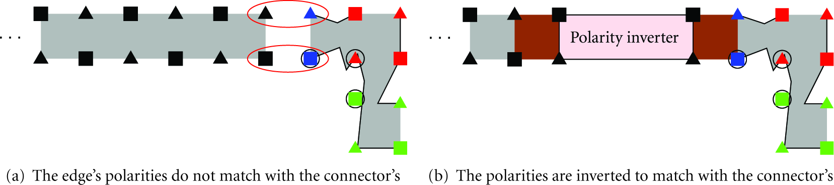
A polarity inverter structure may be needed to invert the polarity of the edge to connect the edge and 3-way connector.

Therefore, referring to Figure 9, we introduce a structure called a polarity inverter and denoted as $S_{p} = (A_{p}, N_{p})$ to invert the polarity. $S_{p}$ contains a main structure, $9 \times 1$ rectangles, and two buffers, $1 \times 1$ squares. (The purpose of the buffers is to ensure $S_{e}$ satisfies the requirement that nonconnected port nodes do not cover any point, except the vertices, of the connection patches, that is, precondition 27(ii).) Similar to edge structures, a polarity inverter use its endpoint pairs, that is, ${n_{i}, n_{i + 1}}$ and ${n_{j}, n_{j + 1}}$ in Figure 9, as ports.

Figure 9

A structure for inverting the polarity of the edge. After distance 11, the polarities are inverted compared with a normal edge.

The distance between two nearby column-pairs of the main structure is $9 / 10$ . Thus, the polarities are inverted compared with a normal edge of the same length. With the polarities inverted, the polarity requirements for vertices of a connection patch can be satisfied as shown in Figure 8(b).

Of course, the structure $S_{p} = (A_{p}, N_{p})$ also satisfies the following lemma. The proof is similar to variable structures and is given in Appendix F.

Lemma 14.

The structure $S_{p} = (A_{p}, N_{p})$ shown in Figure 9 is well aligned and well behaved.

Definition 15.

For a given variable structure $S_{v}$ , an n-way connector $S_{c}$ is called an associated connector of $S_{v}$ if $S_{c}$ is connected to $S_{v}$ via an edge structure. Furthermore, the partition $P_{i}$ of $S_{c}$ where $S_{v}$ is connected to is called an associated partition of $S_{v}$ . Similarly, the edges, polarity inverters, and connection patches used to connect $S_{v}$ and $S_{c}$ are called associated connection edges, associated polarity inverters, and associated connection patches of $S_{v}$ , respectively.

For the ith variable, $v_{i}$ , let $N V_{i}$ :

be the set of nodes in the corresponding variable structures $S_{v_{i}}$ ,

N E_{i}

be the set of nodes in all the associated edge structures of $S_{v_{i}}$ ,

N I_{i}

be the set of nodes in all the associated polarity inverters of $S_{v_{i}}$ ,

N C_{i}

be the set of nodes in all the associated n-way connectors of $S_{v_{i}}$ ,

N P_{i}

be the set of nodes in all the associated partitions of $S_{v_{i}}$ ,

A V_{i}

be the shaded region of $S_{v_{i}}$ ,

A E_{i}

be the union of the shaded region from all the associated edge structures of $S_{v_{i}}$ ,

A I_{i}

be the union of the shaded region from all the associated polarity inverters of $S_{v_{i}}$ ,

A C_{i}

be the union of the shaded region from all the associated n-way connectors of $S_{v_{i}}$ ,

A C P_{i}

be the union of the shaded region from all the associated connection patches of $S_{v_{i}}$ .

Definition 16.

Let $N_{i} = N V_{i} \cup N E_{i} \cup N I_{i} \cup N C_{i}$ , $A_{i} = A V_{i} \cup A E_{i} \cup A I_{i} \cup A C_{i} \cup A C P_{i}$ , and $T_{i} = (A_{i}, N_{i})$ . We call the composite structure $T_{i}$ the territory of the ith variable. Furthermore, let $N_{i}^{'} = N V_{i} \cup N E_{i} \cup N I_{i} \cup N P_{i}$ . The nodes in $N_{i}^{'}$ are the pieces of the ith variable. Note that $N P_{i} \cap N P_{j} = \emptyset if i \neq j$ , and thus $N_{i}^{'} \cap N_{j}^{'} = \emptyset if i \neq j$ .

Note that $T_{i}$ represents the ith variable and all clauses it belongs to as shown in Figure 10. It is not difficult to layout each structure on the plane and make variable structures and connectors far enough to prevent unwanted interactions between nearby structures, that is, structures are least interactively connected. Consequently, we have the following lemma which states that, for a given variable, its territory is partially well behaved on the set of its pieces.

Figure 10

The territory, $T_{i}$ , of the variable $v_{i}$ includes variable structure $S_{v_{i}}$ and all associated edge structures, patches, inverters, and connectors. The nodes enclosed in dashed line are pieces of $v_{i}$ .

Lemma 17.

If all the associated structures of the variable structure $S_{v_{i}}$ are least interactively connected, the territory $T_{i}$ is partially well-behaved on $N_{i}^{'}$ .

Proof.

Since structures are least interactively connected, this lemma can be proved by Lemmas 8, 9(i), 14, and Connection Lemma. The fact that $2 \leq | c | \leq 3$ for each clause c is the key to ensure precondition (ii) of Connection Lemma is satisfied for Connection Lemma being applicable. The complete proof is given in Appendix G.

After introducing the structures and their properties, we can define an equivalent MUDC problem with the geometry, MUDC(B), for a given boolean formula, B, in P3SAT by replacing the variables, clauses, and edges of the bipartite graph $G_{B}$ with their corresponding structures. Denote that

$N V$ :

is the set of nodes in all the variable structures,

N E

is the set of nodes in all the edge structures,

N I

is the set of nodes in all the polarity inverters,

N C

is the set of nodes in all the n-way connectors,

A V

is the union of the shaded region from all the variable structures,

A E

is the union of the shaded region from all the edge structures,

A I

is the union of the shaded region from all the polarity inverters,

A C

is the union of the shaded region from all the n-way connectors,

A C P

is the union of the required connection patches.

Let $MUDC (B) = (A_{B}, N_{B})$ with $A_{B} = A V \cup A E \cup A I \cup A C \cup A C P$ and $N_{B} = N V \cup N E \cup N I \cup N C$ , and $K = | N_{B} | / 2$ . Hence, we have the following claim. Note that it is not difficult to prove that the construction from B to MUDC(B) can be done in polynomial time.

Claim B is satisfiable if and only if MUDC(B) has a UDC with cardinality K.

Note that the key to the backward direction of the proof is Lemma 17; that is, for a given variable, its territory is partially well behaved on the set of its pieces. Lemma 17 will be used to derive, that if MUDC(B) has a UDC with cardinality K, then, for each variable, half of its pieces with same polarity needs to be active to unit-disk cover its territory. Therefore, each variable could be assigned true or false based on the polarity of its active pieces.

4.3. Proof of the Claim

Proof.

⇒ For each $N_{i}^{'}$ , choose the nodes with the polarity which is the same as the assignment of the ith variable in a given satisfying instance of B. Obviously, only $| N | / 2 = K$ nodes are picked. By Lemmas 8, 14, and 10, $A V$ , $A E$ , $A I$ , and $A C P$ are covered. Furthermore, since B is satisfiable, at least one header node of each n-way connector is active. By Lemma 9(iii), $A C$ is covered. Thus MUDC(B) has a UDC with cardinality K.

⇐ Let MUDC(B) have a UDC $U \subseteq N$ with $| U | = K$ . We will show that this set must look right.

From Lemmas 8, 9(i), and 14, we know that the cardinality of an MUDC of a variable structure, edge structure, n-way connector, or polarity inverter is half the number of the nodes in the structure. Since all structures in $MUDC (B)$ are least interactively connected and $| U | = | N | / 2$ , it is not difficult to derive that, for the ith variable structure, $U \cap N_{i}$ is an MUDC of $T_{i}$ by removing nonassociated edge structures of $T_{i}$ one by one and Lemma 12.

From Lemma 17 and $N_{i}^{'} \subseteq N_{i}$ , $U \cap N_{i}^{'}$ only contains the nodes with the same polarity. Thus, the ith variable could be assigned true or false based on the polarity of the nodes in $U \cap N_{i}^{'}$ . Finally, since at least one header node of each n-way connector must be active from Lemma 9(ii), the corresponding clause will be true.

5. Extensions of MUDC

MUDC can be easily extended to the following two more general cover problems, which require each location to be unit-disk covered by predefined number of nodes. These problems regard the quality of various services of sensor network applications such as surveillance, object tracking, and fault tolerance.

Problem 18 (Minimum Unit-Disk k-Cover, MUDKC).

Given a geometry $(A, N)$ and two positive integers k and K, determine whether there is a subset $U \subseteq N$ with $| U | \leq K$ such that $for all x \in A, | {u \in U | x \in disk (u)} | \geq k$ ; that is, x is unit-disk covered by at least k nodes in U.

Problem 19 (Minimum Unit-Disk Multicover, MUDM).

Given a geometry $(A, N)$ , a quality of surveillance function $q : A \to ℤ^{+}$ , and a positive integer K, determine whether there is a subset $U \subseteq N$ with $| U | \leq K$ such that $for all x \in A, | {u \in U | x \in disk (u)} | \geq q (x)$ ; that is, x is unit-disk covered by at least $q (x)$ nodes in U.

We may also consider connectivity and have the following problem.

Problem 20 (Minimum Connected Unit-Disk Cover, MCUDC).

Given a geometry $(A, N)$ , a positive number $R_{c} \in ℝ^{+}$ , and a positive integer K, determine whether there is a subset $U \subseteq N$ with $| U | \leq K$ such that $A \subseteq disk (U)$ and the graph $G_{c} = {U, E_{c}}$ is connected. Here $E_{c} = {(n, n^{'}) | d (n, n^{'}) \leq R_{c}}$ .

Furthermore, under many environmental data sampling applications, instead of full coverage, a predefined percentage of coverage is required for achieving energy efficiency and preciseness of sampling. The objective of the following problem is to find as few nodes as possible to achieve the coverage requirements.

Problem 21 (Minimum Unit-Disk Partial Cover, MUDPC).

Given a geometry $(A, N)$ , a positive number r with $0 \leq r \leq 1$ , and a positive integer K, determine whether there is a subset $U \subseteq N$ with $| U | \leq K$ such that $(area (disk (U))) / area (A) \geq r$ . Here the function $area (\cdot)$ gives the area of a given region.

By the NP-completeness of MUDC, it is easy to derive the complexity of the above problems.

Corollary 22.

MUDKC, MUDM, MCUDC, and MUDPC are NP-complete.

Proof.

Note that every instance of MUDC can be viewed as an instance of MUDKC, MUDM, or MUDPC simply by letting $k = 1$ , $q (x) = 1 for all x \in A$ , or $r = 1$ , respectively. Thus MUDC is just a restricted version of these problems, and their NP-completeness follows by trivial transformations from MUDC.

For the geometry, MUDC(B), described in the NP-completeness proof of MUDC, it is obvious that, for any UDC of $A_{B}$ , the distance between an active node and its closest active node is less than 2. Thus, it is not difficult to prove that if $R_{c} \geq 2$ , $G_{c}$ is connected. That is, MUDC is just a restricted version of MCUDC with $R_{c} \geq 2$ , and the $N P$ -completeness of MCUDC follows by a trivial transformation from MUDC.

6. Arc Sampling Algorithm for Reducing MUDC to MSC

As stated earlier, MUDC may be solved by partitioning the region A into disjoint sectors [20]. Consequently, MUDC is reduced to MSC and many well-known algorithms can be applied, for example, the greedy algorithm is the best approximation algorithm and the approximation factor is well known.

To identify necessary sectors is a key factor to whether the solutions found by the algorithms for the transformed MSC are valid, that is, the solutions are disk covers of the original MUDC. A naive approach for partitioning is to sample A at uniform spacings in a grid pattern; then the sampling points covered by the same set of nodes would be grouped into one sector. With enough resolution, all necessary sectors can be successfully identified at the expense of computation time.

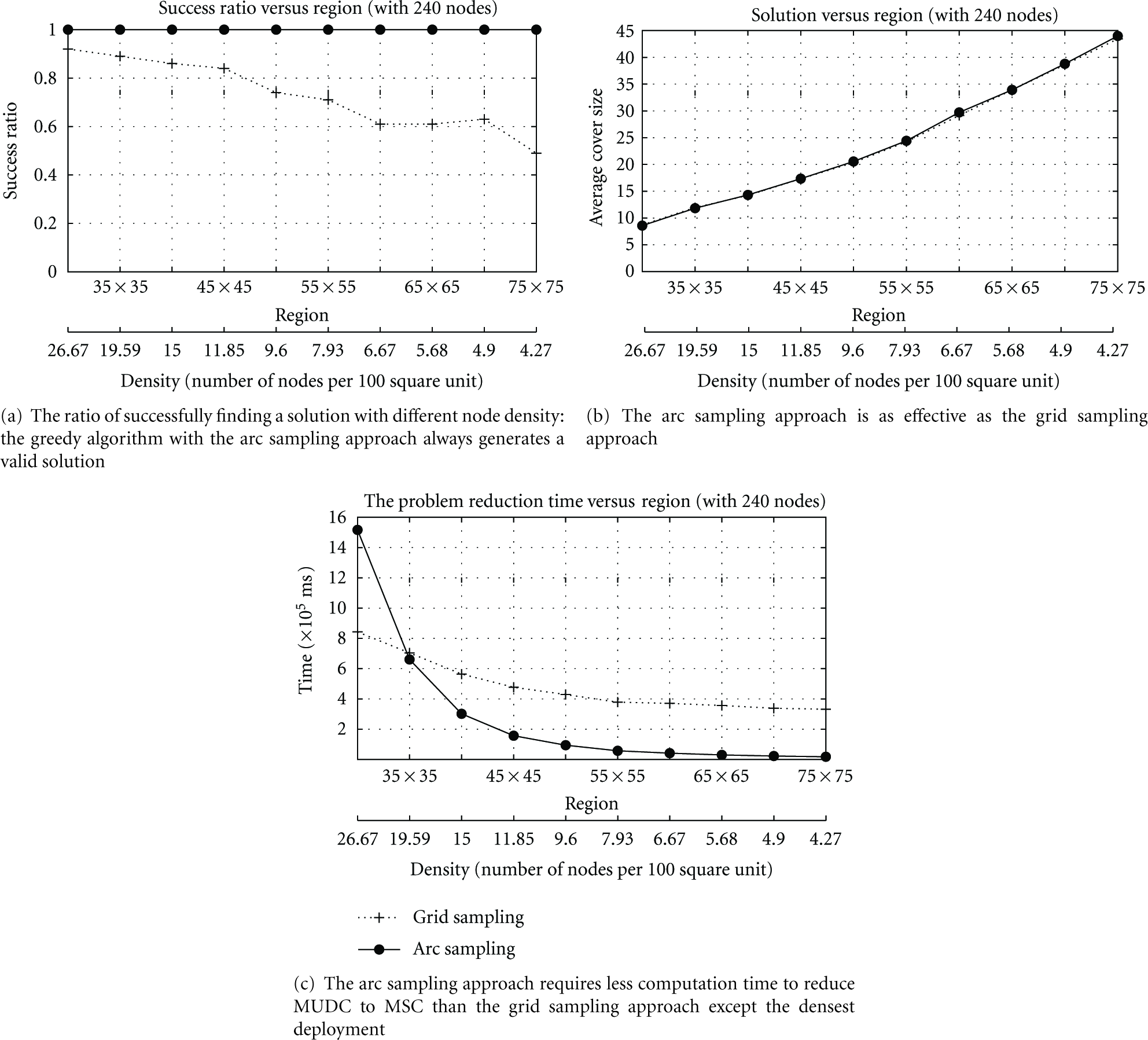
However, to determine a good resolution may be difficult. For example, Figure 11 shows that inappropriately increasing resolution may not necessarily find a valid solution, and Figure 13(a) illustrates that the ratio of successfully finding a valid solution decreases as the node density decreases. Therefore, we propose an arc sampling approach which is inspired by the theorem of the paper [32], that is, A is covered if and only if the perimeter of each node's sensing region is covered. (Several special cases including boundary are also discussed in [32].)

Figure 11

The solution found at different sampling intervals. Increasing resolution may not necessarily find a valid solution.

Consider the node n with its neighbors, that is, the nodes with distance not greater than 2 from n. As illustrated in Figure 12, n's perimeter is divided into disjoint arcs by its neighbors' perimeters and the boundary of A. It is obvious that all points of each disjoint arc in A are covered by the same set of nodes. Thus, we can simply choose a point such as the midpoint from each arc in A, for example, $χ_{2}$ from arc $\hat{α_{2} α_{3}}$ , as a sampling point. Note that if n's perimeter cannot be divided, n's perimeter (and thus A) is not covered [32], as indicated in Lines 7~9 of Algorithm 1. From the earlier mentioned theorem of the paper [32], it is easy to derive that A is covered if and only if all these sampling points are covered. Thus, the solutions of the $M S C$ transformed by this arc sampling approach are always valid.

Algorithm 1: Arc sampling algorithm.

Input: ( $A, N$ )

Output: a set $Ξ$ of sampling points

(1) $Ξ \leftarrow \emptyset$

(2) for all $n_{i} \in N$ do

(3) $Γ \leftarrow P (n_{i}) \cap \partial A$

(4) for all $n_{j} \in N$ such that $d (n_{i}, n_{j}) \leq 2$ do

(5) $Γ \leftarrow Γ \cup (P (n_{i}) \cap P (n_{j}))$

(6) end for

(7) if $Γ = \emptyset$ then

(8) exit $/^{*}$ A is not covered by N. */

(9) end if

(10) List $L \leftarrow$ the points in $Γ$ sorted by their azimuth

angles on the polar coordinate system

with reference to $n_{i}$

(11) for all $α_{i} ϵ L$ such that $1 \leq i < | Γ |$ do

(12) $Ξ \leftarrow Ξ \cup {χ | χ is the midpoint of \hat{α_{i} α_{i + 1}} and χ \in$

$A}$

(13) end for

(14) $Ξ \leftarrow Ξ \cup {χ | χ is the midpoint of \hat{α_{| Γ |} α_{1}} and χ \in$

$A}$

(15)end for

Figure 12

Each arc in A, that is, $\hat{α_{2} α_{3}}$ , $\hat{α_{3} α_{4}}$ , or $\hat{α_{4} α_{5}}$ , is covered by the same set of nodes. Hence, we can simply use a point, for example, the midpoint marked as a cross, from each arc as a sampling point. Here $\partial A$ represents the boundary of A.

Figure 13

The experiment results show that the arc sampling approach is effective and effcient for reducing MUDC to MSC.

The arc sampling algorithm is shown in Algorithm 1. Here $P (n) = {x | d (n, x) = 1}$ is the perimeter of n. The outer loop between Lines 2 and 15 will run $| N |$ times. The average time complexity for a node to find all its perimeter intersections with neighbors, that is, Lines 4~6, is $O (4 π d)$ . Here $d = | N | / area (A)$ is the density of nodes. Note that each node has average $4 π d$ neighbors and thus $8 π d$ disjoint arcs. Hence, the sorting in Line 10 could be implemented in $O (8 π d \cdot \log 8 π d) = O (d \log d)$ time. In addition, the time complexity of finding the midpoints, that is, Lines 11~14, is $O (8 π d)$ . Thus the overall time complexity of Algorithm 1 is $O (| N | d \log d)$ or $O (area (A) \cdot d^{2} \log d)$ . On the other hand, it is not difficult to derive that the time complexity of finding all sampling points is $O (area (A) / a)$ for the grid sampling approach. Here a is the area of each grid. Together with Figure 13(a), we may conclude that the arc sampling approach will perform more efficiently than the grid sampling approach, particularly with low density of nodes.

We conducted an experiment to compare the grid sampling and the arc sampling approaches. In the experiment, there are 240 nodes deployed uniformly in a square region ranging from $30 \times 30$ to $75 \times 75$ . The radius of the sensing range is 10. The sampling interval of the grid sampling approach is 0.1. After transforming to $M S C$ , the greedy algorithm is used to find the approximated solution. Each result is the average of 100 random deployments.

Figure 13(b) shows the effectiveness of the arc sampling approach. The solutions from both approaches have almost same sizes, that is, same number of nodes. However, Figure 13(a) shows that not every solution obtained from the grid sampling approach is valid. Figure 13(c) illustrates that the arc sampling approach requires less computation time to reduce MUDC to MSC than the grid sampling approach except the densest deployment. Thus, the arc sampling approach is effective and efficient for reducing MUDC to MSC.

7. Decentralized Polynomial Approximation Algorithms

Algorithm 1 and the greedy algorithm may not be suitable for all practical sensor network applications, since it is a centralized algorithm at the cost of potentially excessive communication across the whole network and communication accounts for the majority of energy consumption. The communication power consumption increases with number of nodes and internode distances, so it is not well scalable. Unless the nodes involving in the communication and computation have enough resources, the algorithm may not complete successfully.

Thus, we present a decentralized algorithm in which nodes only require local information by using the divide and conquer technique described in [42] and derive its approximation factor. Furthermore, if the maximum node density is fixed, we may design a constant approximation factor algorithm by using the similar technique. (Note that MUDC remains NP-complete even with fixed maximum node density. It could be easily proved from the fact that the density of MUDC(B) in the NP-completeness proof of MUDC is bounded by a constant.)

7.1. Decentralized Greedy Approximation Algorithm

The proposed algorithm for the instance $(A, N)$ proceeds as follows. (1)

Use Algorithm 1 to determine sampling points.

(2)

Divide A into vertical strips with width being the diameter of the sensing region, that is, 2. Each strip is left closed and right open. Number strips from left to right. There are total I strips.

(3)

Divide each strip into cells with length being the diameter of the sensing region. Each cell is bottom closed and top open. Number cells from bottom to top. Denote the jth cell of the ith strip as $C_{i, j}$ . There are total J cells for each strip.

(4)

Apply the greedy algorithm to each cell, that is, select a node that covers the maximum number of uncovered sampling points in the cell. Denote the solution of $C_{i, j}$ as $SO L_{C_{i, j}}$ .

(5)

Output the solution $SO L_{A} = ⋃_{\begin{smallmatrix} 1 \leq i \leq I \\ 1 \leq j \leq J \end{smallmatrix}} SO L_{C_{i, j}}$ .

Figure 14(a) illustrates that A is divided into $2 \times 2$ cells. Note that each sampling point is located in exactly one cell. This algorithm requires that geometric information of A and cells are known a priori to each node and each node's location can be determined after deployment.

Figure 14

Divide and conquer: (a) The monitored region A (enclosed in heavy line) is divided into $2 \times 2$ cells. (b) $C_{i, j}$ (enclosed in heavy line) and its repository $𝔭_{i, j}$ (enclosed in thin line)—the solid lines and dashed lines represent closed and open boundaries. Note that the distance between any two points in $𝔭_{i, j}$ does not exceed $(2 + 2 \sqrt{2})$ .

For each cell $C_{i, j}$ , we define its repository $𝔭_{i, j} = {x | \exists y \in C_{i, j}, d (x, y) \leq 1}$ . As illustrated in Figure 14(b), $𝔭_{i, j}$ is the region containing all nodes that may cover the sampling points in $C_{i, j}$ . Hence, in Step 4, the greedy algorithm is applied to the nodes in each cell's repository and can be implemented in $O (n_{r p}^{2} \log n_{r p})$ , where $n_{r p}$ is the maximum number of nodes in a repository. Furthermore, Figure 14(b) also illustrates that a node does not need to communicate with others further than $(2 + 2 \sqrt{2})$ times of the sensing radius. Thus, this approach is more scalable than the centralized greedy algorithm.

Theorem 23.

The above algorithm has an approximation factor $4 O (\log m)$ . (Though $4 O (\log m)$ can be written as $O (\log m)$ by definition, we explicitly write it out to emphasize the approximation factor of the decentralized algorithm is four times the approximation factor of the centralized algorithm.) Here m is the maximum number of sampling points covered by a single node.

Proof.

The theorem is the result of the shifting lemma in [42]. The proof proceeds as follows.

For $A^{'} \subseteq A$ , denote that $OP T_{A^{'}}$ is the optimum solution to cover the sampling points in $A^{'}$ . That is, $OP T_{C_{i, j}}$ is the optimum solution for $C_{i, j}$ , $OP T_{⋃_{j} C_{i, j}}$ is the optimum solution for the ith strip, and so forth. Thus, from Step 4, $| SO L_{C_{i, j}} | \leq O (\log m_{i, j}) \cdot | OP T_{C_{i, j}} |$ . Here $m_{i, j}$ is the maximum number of sampling points in $C_{i, j}$ covered by a single node.

Consider the ith strip, and define the following disjoint subsets of $OP T_{⋃_{j} C_{i, j}}$ :

$OP T^{(j)}$ be the set of nodes that only cover the sampling points in $C_{i, j}$ ,

$OP T^{(j, j + 1)}$ be the set of nodes that cover both the sampling points in $C_{i, j}$ and $C_{i, j + 1}$ .

Note that since the length of cells is the diameter of the sensing region, the union of the above disjoint subsets is $OP T_{⋃_{j} C_{i, j}}$ . Hence, $| OP T_{⋃_{j} C_{i, j}} | = \sum_{1 \leq j \leq J} | {OPT}^{(j)} | + \sum_{1 \leq j \leq J - 1} | {OPT}^{(j, j + 1)} |$ . Besides, it is obvious that $OP T^{(j - 1, j)} \cup OP T^{(j)} \cup OP T^{(j, j + 1)}$ covers all sampling points in $C_{i, j}$ . (Here $OP T^{(0,1)} = \emptyset$ and $OP T^{(J, J + 1)} = \emptyset$ .) Thus, $| OP T_{C_{i, j}} | \leq | OP T^{(j - 1, j)} \cup OP T^{(j)} \cup OP T^{(j, j + 1)} | = | OP T^{(j - 1, j)} | + | OP T^{(j)} | + | OP T^{(j, j + 1)} |$ . Therefore, it can easily be derived that

\begin{matrix} \sum_{1 \leq j \leq J} | OP T_{C_{i, j}} | & \leq | OP T_{⋃_{j} C_{i, j}} | \\ + \sum_{1 \leq j \leq J - 1} | OP T^{(j, j + 1)} | \\ \leq 2 \cdot | OP T_{⋃_{j} C_{i, j}} | . \end{matrix}

(1)

Similarly, it can easily be derived that

\begin{matrix} \sum_{1 \leq i \leq I} | OP T_{⋃_{j} C_{i, j}} | \leq 2 \cdot | OP T_{A} |, \end{matrix}

(2)

and then

\begin{matrix} \sum_{\begin{matrix} 1 \leq i \leq I \\ 1 \leq j \leq J \end{matrix}} | OP T_{C_{i, j}} | \leq 4 \cdot | OP T_{A} | . \end{matrix}

(3)

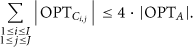
Consequently,

\begin{matrix} | SO L_{A} | & \leq \sum_{\begin{matrix} 1 \leq i \leq I \\ 1 \leq j \leq J \end{matrix}}^{} | SO L_{C_{i, j}} | \\ \leq \sum_{\begin{matrix} 1 \leq i \leq I \\ 1 \leq j \leq J \end{matrix}}^{} O (\log m_{i, j}) | OP T_{C_{i, j}} | \\ \leq O (\log m) \cdot \sum_{\begin{matrix} 1 \leq i \leq I \\ 1 \leq j \leq J \end{matrix}}^{} | OP T_{C_{i, j}} | \\ \leq 4 O (\log m) \cdot | OP T_{A} | . \end{matrix}

(4)

Note that, obviously, $\max_{i, j} {m_{i, j}} \leq m$ .

7.2. Constant Approximation Factor Algorithm with Fixed Maximum Density

When the maximum node density, denoted as d, is fixed, the similar divide and conquer technique can be used to derive a constant approximation factor algorithm.

The algorithm is almost the same as the previous one except Step 4, which will be modified as follows:

(4) Apply an exhaustive search for optimum solution to each cell. Denote the solution of $C_{i, j}$ as $SO L_{C_{i, j}}$ .

Theorem 24.

The above algorithm has a constant approximation factor 4.

Proof.

Note that the number of nodes in each cell's repository is at most $⌈ area (𝔭_{i, j}) \cdot d ⌉ = ⌈ (12 + π) d ⌉$ . (Refer to Figure 14(b); the area of each repository is $(12 + π)$ .) Thus, the time complexity of the exhaustive search is at most $2^{⌈ (12 + π) d ⌉}$ for each cell. Since d is fixed, an optimum solution for each cell can be found with a constant time complexity. Since $| SO L_{C_{i, j}} | = | OP T_{C_{i, j}} |$ , from (3), we have

\begin{matrix} | SO L_{A} | \leq \sum_{\begin{matrix} 1 \leq i \leq I \\ 1 \leq j \leq J \end{matrix}}^{} | SO L_{C_{i, j}} | \leq 4 \cdot | OP T_{A} | . \end{matrix}

(5)

7.3. Performance Evaluation

We conducted various simulations to evaluate the proposed algorithms. In Figure 15, nodes are deployed uniformly within a $30 \times 30$ square region. Figures 15(a) and 15(b) show the solution size and execution time for various sensing ranges in which there are 25 nodes. The optimum solution $OPT$ is found by exhaustive searching. $GRD$ denotes the solution by using Algorithm 1 and the greedy algorithm. $deGRD$ and $deOPT$ represent the algorithms described in Sections 7.1 and 7.2 respectively. The cover size decreases as the sensing radius increases, since each node can cover a larger region. $GRD$ and $deOPT$ have similar performance in terms of cover size and execution time. Furthermore, $deGRD$ generates the largest cover size, on average $48 %$ more than $OPT$ , $22.7 %$ more than $GRD$ , or $21 %$ more than $deOPT$ , but requires the least execution time, on average $0.01 %$ of $OPT$ , $22.7 %$ of $GRD$ , or $17.8 %$ of $deOPT$ .

Figure 15

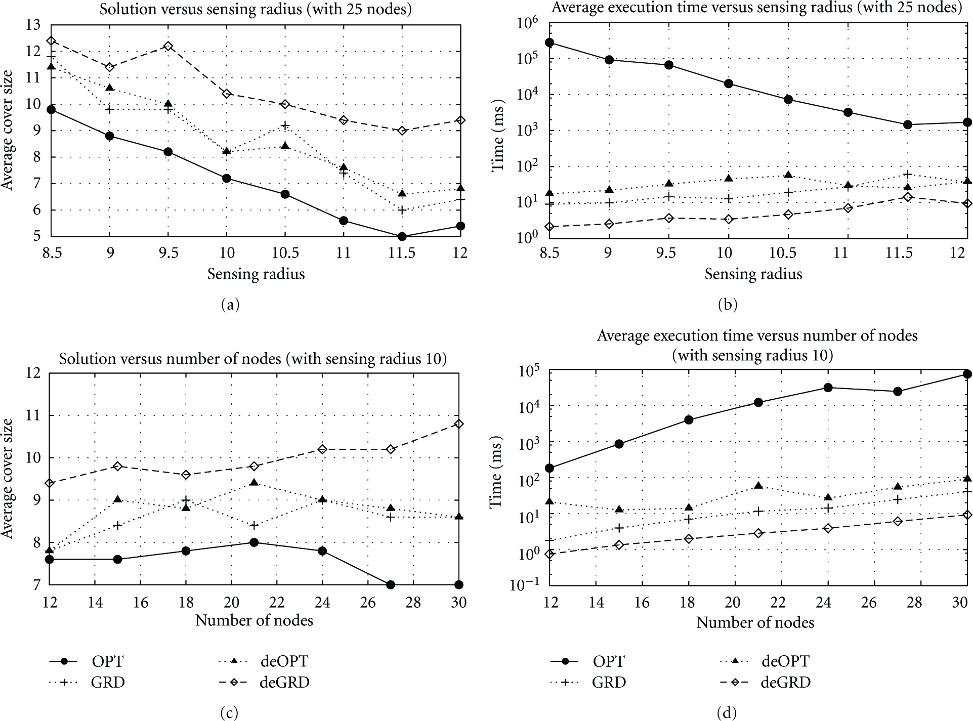
Performance evaluation: the nodes are deployed uniformly within a $30 \times 30$ square region.

Figures 15(c) and 15(d) indicate the solution size and execution time for various number of nodes in which the sensing radius is fixed at 10. The cover size does not change significantly as the number of nodes increases, since the sensing region of each node does not change. $GRD$ and $deOPT$ have similar cover size, but $deOPT$ requires more execution time than $GRD$ . Similarly, $deGRD$ generates the largest cover size, on average $32 %$ more than $OPT$ , $17 %$ more than $GRD$ , or $14 %$ more than $deOPT$ , in the least time, on average $0.017 %$ of $OPT$ , $16.7 %$ of $GRD$ , or $9.5 %$ of $deOPT$ .

We also considered the scenario in which nodes are deployed in a Gaussian distribution with the peak located at the center of A and the variance 15, and the results are illustrated in Figure 16. Here A is a $30 \times 30$ square region. In Figures 16(a) and 16(b), the number of nodes is 25 and the sensing radius varies between 8.5 and 12. $deGRD$ generates the largest cover size, on average $50 %$ more than $OPT$ , $18.7 %$ more than $GRD$ , or $26 %$ more than $deOPT$ , but requires the least execution time, on average $0.019 %$ of $OPT$ , $21.7 %$ of $GRD$ , or $10 %$ of $deOPT$ .

Figure 16

Performance evaluation: the nodes are deployed in a Gaussian distribution with the peak located at the center of A and the variance 15. Here A is a 30×30 square region.

Furthermore, in Figures 16(c) and 16(d), the sensing radius is fixed at 10 and the number of nodes varies between 12 and 30. Similarly, $deGRD$ generates the largest cover size, on average $40 %$ more than $OPT$ , $13.1 %$ more than $GRD$ , or $20.6 %$ more than $deOPT$ , in the least time, on average $0.03 %$ of $OPT$ , $20.8 %$ of $GRD$ , or $8.2 %$ of $deOPT$ . For most of cases, $deOPT$ has smaller cover sizes than $GRD$ in this scenario.

8. Conclusion

In this paper, we consider the complexity of MUDC, the Minimum Unit-Disk Cover problem. This problem has applications in extending the sensor network lifetime by selecting minimum number of nodes to fully cover a geometric connected region of interest and putting the remaining nodes in power saving mode. MUDC is a restricted version of MSC where the sensing region of each node is a unit-disk and the monitored region is geometric connected, a well-adopted network model in many works of the literature.

To prove the hardness of MUDC, we construct various structures to represent variables and edges of a given P3SAT instance's bipartite graph $G_{B}$ . With the well-aligned and partially well-behaved properties of these structures, we illustrate that the structures can be unit-disk covered with half of nodes. Furthermore, we introduce the n-way connectors to represent clauses, which can be unit-disk covered with half of its nodes if and only if the corresponding clauses have true assignments. Finally, we discuss how complex structures can be constructed by connecting simpler structures while still preserving these properties, that is, via the least interactive connection. Thus, we prove that P3SAT can be directly reduced to MUDC in polynomial time, and obtain the NP-completeness proof of MUDC.

We also discuss several optimum problems with various coverage constraints introduced by different sensing applications. These problems are extensions of MUDC, and their NP-completeness proofs are presented as a corollary.

We propose the arc sampling algorithm which may effectively and efficiently reduce MUDC to MSC, and many well-known algorithms can be applied to find approximated solutions. We also propose a decentralized algorithm with a guaranteed performance. The algorithm requires only local communication, that is, a node does not need to communicate with others further than $(2 + 2 \sqrt{2})$ times of the sensing radius. Thus, this approach is scalable. Furthermore, we present an algorithm with a constant approximation factor 4 if the maximum node density is fixed. Finally, we provide simulation results to evaluate the proposed algorithms and the optimum algorithm in uniform and Gaussian deployment networks. The results show that $deOPT$ may have smaller cover size than $GRD$ at the cost of more execution time. In addition, $deGRD$ generates the largest cover size in the least time.

Footnotes

Appendices

Acknowledgment

This research was supported by National Science Council (NSC), Taiwan, under Grant NSC 99-2221-E-194-021. The author gratefully acknowledges this support.

References

Akyildiz

I. F.

Sankarasubramaniam

Cayirci

Wireless sensor networks: a survey

Computer Networks 2002 38 4 393 422

2-s2.0-0037086890

10.1016/S1389-1286(01)00302-4

ANSI/IEEE, Standard 802.11

Wireless LAN Medium Access Control(MAC) and Physical Layer(PHY) specifications

1999

Stine

J. A.

Veciana

G. D.

Improving energy efficiency of centrally controlled wireless data networks

Wireless Networks 2002 8 6 681 700

2-s2.0-0036847412

10.1023/A:1020379326558

Srinivas

Modiano

Minimum energy disjoint path routing in wireless Ad-hoc networks

Proceedings of the 9th Annual International Conference on Mobile Computing and Networking

2003

San Diego, Calif, USA

ACM Press

122 133

Sankar

Liu

Maximum lifetime routing in wireless Ad-hoc networks

Proceedings of the IEEE Infocom

March 2004

Hong Kong, China

2-s2.0-8344234971

Singh

Raghavendra

C. S.

Stepanek

Power-aware broadcasting in mobile Ad Hoc networks

Proceedings of the 10th Annual IEEE International Symposium on Personal Indoor and Mobile Radio Communications

September 1999

Osaka, Japan

Stojmenovic

Power-aware broadcasting and activity scheduling in Ad Hoc wireless networks using connected dominating sets

Wireless Communications and Mobile Computing 2003 3 4 425 438

2-s2.0-13244278088

10.1002/wcm.125

Wieselthier

J. E.

Nguyen

G. D.

Ephremides

Multicasting in energy-limited Ad-hoc wireless networks

Proceedings of the IEEE Military Communications Conference

October 1998

723 729

2-s2.0-0032310335

Liang

Approximate minimum-energy multicasting in wireless Ad Hoc networks

IEEE Transactions on Mobile Computing 2006 5 4 377 387

2-s2.0-33644662084

10.1109/TMC.2006.1599406

10.

Topology control for multihop packet radio networks

IEEE Transactions on Communications 1993 41 10 1474 1481

2-s2.0-0027677867

10.1109/26.237882

11.

Wattenhofer

Bahl

Wang

Y.-M.

Distributed topology control for power efficient operation in multihop wireless Ad Hoc networks

Proceedings of the IEEE Infocom

April 2001

Anchorage, AK, USA

1388 1397

12.

Shah

R. C.

Rabaey

J. M.

Energy aware routing for low energy Ad Hoc sensor networks

Proceedings of the IEEE Wireless Communication and Networking Conference

March 2002

Orlando, Fla, USA

13.

Chang

J.-H.

Tassiulas

Maximum lifetime routing in wireless sensor networks

IEEE/ACM Transactions on Networking 2004 12 4 609 619

2-s2.0-4644360171

10.1109/TNET.2004.833122

14.

Schurgers

Tsiatsis

Ganeriwal

Srivastava

Optimizing sensor networks in the energy-latency-density design space

IEEE Transactions on Mobile Computing 2002 1 1 70 80

2-s2.0-3042785191

10.1109/TMC.2002.1011060

15.

Nama

Mandayam

Sensor networks over information fields: optimal energy and node distributions

Proceedings of the IEEE Wireless Communications and Networking Conference

March 2005

1842 1847

2-s2.0-24944500053

16.

Raghunathan

Schurgers

Park

Srivastava

M. B.

Energy-aware wireless microsensor networks

IEEE Signal Processing Magazine 2002 19 2 40 50

2-s2.0-0036503188

10.1109/79.985679

17.

Meguerdichian

Koushanfar

Potkonjak

Srivastava

M. B.

Coverage problems in wireless Ad-hoc sensor networks

Proceedings of the IEEE Infocom

April 2001

Anchorage, Alaska, USA

1380 1387

2-s2.0-0034997317

18.

Niculescu

Nath

Ad hoc positioning system (APS) using AOA

Proceedings of the 22nd Annual Joint Conference on the IEEE Computer and Communications Societies

April 2003

San Franciso, Calif, USA

1734 1743

2-s2.0-0041973656

19.

Tseng

Y.-C.

Kuo

S.-P.

Lee

H.-W.

Huang

C.-F.

Location tracking in a wireless sensor network by mobile agents and its data fusion strategies

Proceedings of the 2nd International Symposium on Information Processing in Sensor Networks

April 2003

Palo Alto, Calif, USA

625 641

20.

Slijepcevic

Potkonjak

Power efficient organization of wireless sensor networks

Proceedings of the IEEE International Conference on Communications

June 2001

Helsinki, Finland

472 476

21.

Funke

Kesselman

Kuhn

Lotker

Segal

Improved approximation algorithms for connected sensor cover

Wireless Networks 2007 13 2 153 164

2-s2.0-33847179510

10.1007/s11276-006-3724-9

22.

Garey

M. R.

Johnson

D. S.

Computers and Intractability: A Guide to the Theory of NP-Completeness 1979 chapter A3

W.H. Freeman and Company

23.

Johnson

D. S.

Approximation algorithms for combinatorial problems

Journal of Computer and System Sciences 1974 9 3 256 278

2-s2.0-0016349356

10.1016/S0022-0000(74)80044-9

24.

Lovász

On the ratio of optimal integral and fractional covers

Discrete Mathematics 1975 13 4 383 390

2-s2.0-0000203509

25.

Chvátal

A greedy heuristic for the set-covering problem

Mathematics of Operations Research 1979 4 3 233 235

26.

Feige

A threshold of in n for approximating set cover

Journal of the ACM 1998 45 4 634 652

2-s2.0-0032108328

27.

Meguerdichian

Koushanfar

Potkonjak

Exposure in wireless Ad-Hoc sensor networks

Proceedings of the 7th Annual International Conference on Mobile Computing and Networking

2001

Rome, Italy

ACM Press

139 150

28.

Meguerdichian

Slijepcevic

Karayan

Potkonjak

Localized algorithms in wireless Ad-Hoc networks: location discovery and sensor exposure

Proceedings of the 2nd ACM International Symposium on Mobile Ad Hoc Networking and Computing

2001

Long Beach, CA, USA

ACM Press

106 116

29.

Gui

Mohapatra

Power conservation and quality of surveillance in target tracking sensor networks

Proceedings of the 10th Annual International Conference on Mobile Computing and Networking

October 2004

Philadelphia, PA, USA

129 143

2-s2.0-11244271384

30.

Tian

Georganas

N. D.

A coverage-preserving node scheduling scheme for large wireless sensor networks

Proceedings of the 1st ACM International Workshop on Wireless Sensor Networks and Applications

2002

Atlanta, Ga, USA

ACM Press

32 41

31.

Carbunar

Grama

Vitek

Carbunar

Redundancy and coverage detection in sensor networks

ACM Transactions on Sensor Networks 2006 2 1 94 128

2-s2.0-33745257022

10.1145/1138127.1138131

32.

Huang

C.-F.

Tseng

Y.-C.

The coverage problem in a wireless sensor network

Proceedings of the 2nd ACM International Conference on Wireless Sensor Networks and Applications

2003

San Diego, Calif, USA

ACM Press

115 121

33.

Zhang

Hou

J. C.

Maintaining sensing coverage and connectivity in large sensor networks

The Wireless Ad Hoc and Sensor Networks 2005 1 89 124

34.

Wang

Xing

Zhang

Pless

Gill

Integrated coverage and connectivity configuration in wireless sensor networks

Proceedings of the 1st International Conference on Embedded Networked Sensor Systems

2003

Los Angeles, Calif, USA

ACM Press

28 39

35.

Gupta

Zhou

Das

S. R.

Connected sensor cover: self-organization of sensor networks for efficient query execution

IEEE/ACM Transactions on Networking 2006 14 1 55 67

36.

Kumar

A. V. S.

Arya

Ramesh

Hardness of set cover with intersection 1

Proceedings of the 27th International Colloquium on Automata, Languages and Programming

2000

London, UK

Springer

624 635

37.

Fowler

R. J.

Paterson

Tanimoto

S. L.

Optimal packing and covering in the plane are NP complete

Information Processing Letters 1981 12 3 133 137

38.

Megiddo

Supowit

K. J.

On the complexity of some common geometric location problems

SIAM Journal on Computing 1984 13 1 182 196

39.

Marathe

M. V.

Radhakrishnan

Harry

Hunt

Ravi

S. S.

Hierarchically specified unit disk graphs

Theoretical Computer Science 1997 174 1-2 23 65

40.

Brönnimann

Goodrich

M. T.

Almost optimal set covers in finite VC-dimension

Discrete & Computational Geometry 1995 14 4 463 479

10.1007/BF02570718

41.

Gonzalez

T. F.

Covering a set of points in multidimensional space

Information Processing Letters 1991 40 4 181 188

10.1016/0020-0190(91)90075-S

42.

Hochbaum

D. S.

Maass

Approximation schemes for covering and packing problems in image processing and Vlsi

Journal of the ACM 1985 32 1 130 136

10.1145/2455.214106

43.

Franceschetti

Cook

Bruck

A geometric theorem for network design

IEEE Transactions on Computers 2004 53 4 483 489

10.1109/TC.2004.1268406

44.

Franceschetti

Cook

Bruck

A Geometric Theorem for Approximate Disk Covering Algorithms

California Institute of Technology, Technical Report ETR035, 2001http://www.paradise.caltech.edu/papers/etr035.pdf

45.

Lichtenstein

Planar formulae and their uses

SIAM Journal on Computing 1982 11 2 329 343

46.

Garey

M. R.

Johnson

D. S.

Computers and Intractability: A Guide to the Theory of NP-Completeness 1979 chapter A9

W.H. Freeman and Company

The Complexity of the Minimum Sensor Cover Problem with Unit-Disk Sensing Regions over a Connected Monitored Region

Abstract

1. Introduction

2. Related Work

2.1. Coverage Problems

2.2. Minimum Sensor Cover Problems

2.3. Related Optimum Problems

3. Preliminaries

Definition 1.

Definition 2.

Problem 3 (MUDC).

Theorem 4.

Problem 5 (Planar 3-SAT, P3SAT).

Definition 6.

Definition 7.

4. NP-Completeness Proof of MUDC

4.1. Structures

Lemma 8.

Proof.

Lemma 9.

Proof.

4.2. Composite Structures

Lemma 10.

Definition 11.

Lemma 12.

Lemma 13 (Connection Lemma).

Lemma 14.

Definition 15.

Definition 16.

Lemma 17.

Proof.

4.3. Proof of the Claim

Proof.

5. Extensions of MUDC

Problem 18 (Minimum Unit-Disk k-Cover, MUDKC).

Problem 19 (Minimum Unit-Disk Multicover, MUDM).

Problem 20 (Minimum Connected Unit-Disk Cover, MCUDC).

Problem 21 (Minimum Unit-Disk Partial Cover, MUDPC).

Corollary 22.

Proof.

6. Arc Sampling Algorithm for Reducing MUDC to MSC

Algorithm 1: Arc sampling algorithm.

7. Decentralized Polynomial Approximation Algorithms

7.1. Decentralized Greedy Approximation Algorithm

Theorem 23.

Proof.

7.2. Constant Approximation Factor Algorithm with Fixed Maximum Density

Theorem 24.

Proof.

7.3. Performance Evaluation

8. Conclusion

Footnotes

Appendices

Acknowledgment

References