Linear Decision Fusion under the Control of Constrained PSO for WSNs

Abstract

A major application of a distributed WSN (wireless sensor network) is to monitor a specific area for detecting some events such as disasters and enemies. In order to achieve this objective, each sensor in the network is required to collect local observations which are probably corrupted by noise, make a local decision regarding the presence or absence of an event, and then send its local decision to a fusion center. After that, the fusion center makes the final decision depending on these local decisions and a decision fusion rule, so an efficient decision fusion rule is extremely critical. It is obvious that the decision-making capability of each node is different owing to the dissimilar signal noise ratios and some other factors, so it is easy to understand that a specific sensor contribution to the global decision should be constrained by this sensor decision-making capability, and, based on this idea, we establish a novel linear decision fusion model for WSNs. Moreover, the constrained particle swarm optimization (constrained PSO) algorithm is creatively employed to control the parameters of this model in this paper and we also apply the typical penalty function to solve the constrained PSO problem. The emulation results indicate that our design is capable of achieving very high accuracy.

1. Introduction

Owing to the low cost and ease of operation, wireless sensor networks are ideal for a wide variety of applications such as environmental monitoring, smart factory instrumentation, intelligent transportation, and remote surveillance [1– 3]. When a WSN is used to monitor an area, each sensor node in the network should collect local observations and send a summary (compressed or partially processed data) to the fusion center. Then the fusion center uses these summaries and a specific decision fusion rule to make the final global decision, as shown in Figure 1.

Figure 1

A typical structure of a decentralized decision fusion system.

Actually, WSN issues such as node deployment, localization, energy-aware clustering, and data aggregation are always considered as optimization problems. An optimization method that requires moderate memory and computational resources and yet produces good results is desirable, especially for implementation on an individual sensor node. Bio-inspired optimization methods are computationally efficient alternatives to analytical methods. Particle swarm optimization (PSO) [4] is a popular multidimensional optimization technique. Ease of implementation, high quality of solutions, computational efficiency, and speed of convergence are the advantages of the PSO. In literatures [5– 9], PSO is used to discover the optimal WSN deployment. Static deployment is a one-time process in which solution quality is more important than fast convergence. PSO suits centralized deployment. Fast PSO variants are necessarily of dynamic deployment, so PSO limits network scalability. Literatures [10– 14] apply PSO for WSN localization. Owing to energy issues, the distributed localization is desirable. Though PSO is appropriate for distributed localization, the choice is influenced by availability of memory on the nodes. Besides, PSO is also used for energy-aware clustering in literatures [15– 17], where clustering is a centralized optimization carried out in a resource-rich base station and optimal clustering has a strong influence on the performance of WSNs. Recently, some researchers have begun to use PSO for WSN data aggregation. As discussed in literature [18], PSO has provided optimization in several aspects of data aggregation as follows.

• (a)

In [19], Wimalajeewa and Jayaweera address the problem of optimal power allocation through constrained PSO. Their algorithm PSO-Opt-Alloc uses PSO to determine optimal-power allocation in the cases of both independent and correlated observations. The objective is to minimize the energy expenditure while keeping the fusion-error probability under a required threshold.

(b)

In [20], Veeramachaneni and Osadciw present a hybrid of ant-based control and PSO (ABC-PSO) for hierarchy and threshold management for decentralized serial sensor networks. PSO is used to determine the optimal thresholds and fusion rules for the sensors while the ant colony optimization algorithm determines the hierarchy of sensor decision communication.

(c)

In [21], Veeramachaneni and Osadciw present a binary multiobjective PSO BMPSO for optimal configuration for multiple sensor networks. PSO is modified to optimize two objectives: accuracy and time. The output of the algorithm is the choice of sensors, individual sensor threshold, and the optimal decision fusion rule.

As mentioned above, data fusion is a distributed repetitive process which is moderately suitable for PSO. Effective data fusion influences overall WSN performance and demands quick-convergence optimization techniques that assure high-quality solutions. Therefore, it is reasonable for us to choose PSO to control the parameters of our fusion rule.

In this paper, we design a linear decision fusion rule. In this rule, a linear equation is used to compute the integrated contribution of all the local decisions, and this equation is made up with local decision weight $k_i$ and all local decisions. Local decision weight $k_i$ can reflect a sensor decision-making capability, and the result of this equation is the summation of all the local sensor contributions. By comparing the result of the linear equation with a threshold ${\lambda }_{\text{g}}$ , the final decision can be made in the fusion center. In order to get the smallest error probability, constrained PSO is employed to find out the optimal local decision weight $k_i$ and the threshold ${\lambda }_{\text{g}}$ .

The rest of the paper is organized as follows. Section 2 discusses the constrained-PSO algorithm briefly. Section 3 describes our linear decision fusion rule in detail. The performance of our fusion rule is evaluated in Section 4, and Section 5 concludes this paper.

2. Brief Introduction of Constrained PSO Algorithm

The particle swarm optimization (PSO) algorithm is a population-based evolutionary computation originally developed by Kennedy and Eberhart [4]. This algorithm does very well in searching throughout a highly multiple modal search space resulting in an optimized solution to an n-dimensional problem. PSO, originally introduced in terms of social and cognitive behavior, is widely used as a bottom-up problem solving method in engineering and computer science.

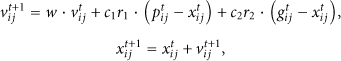
In the basic PSO algorithm, a swarm consists of m particles flying around in an n-dimensional search space. The position of the ith particle at the tth iterations is used to evaluate the particle and represent the candidate solution for the optimization problem. It can be presented as $X_i^t=[x_{i1}^t,x_{i2}^t,\dots ,x_{in}^t]$ , where $x_{ij}^t$ is the position value of the ith particle with respect to the jth dimension $(j=\mathrm{1,2},\dots ,n)$ . During the searching process, the position of a particle is affected by two factors: the best position visited by itself $(p_{\text{best}})$ denoted as $P_i^t=[p_{i1}^t,p_{i2}^t,\dots ,p_{in}^t]$ and the best position of the swarm found so far $(g_{\text{best}})$ denoted as $G^t=[g_1^t,g_2^t,\dots ,g_n^t]$ . The new velocity (denoted as $V_i^t=[v_{i1}^t,v_{i2}^t,\dots ,v_{in}^t]$ ) and the position of particle i at the next iteration are calculated as

$\begin{array}{c}{v}_{ij}^{t+1}=w\cdot v_{ij}^t+c_1{r}_1\cdot \left(p_{ij}^t-x_{ij}^t\right)+c_2{r}_2\cdot \left(g_{ij}^t-x_{ij}^t\right),\\ x_{ij}^{t+1}=x_{ij}^t+v_{ij}^{t+1},\end{array}$

(1)

where w is called the inertia parameter, $c_1$ and $c_2$ are, respectively, cognitive and social learning parameters, and $r_1$ , $r_2$ are random numbers between (0,1). Relying on expressions (1), the particles can fly throughout search space toward $p_{\text{best}}$ and $g_{\text{best}}$ in a navigated way while still exploring new areas by the stochastic mechanism to escape from local optimal. The process for a particle to update its location is as shown in Figure 2.

Figure 2

The process of updating location for each iteration in PSO.

Further, a constrained PSO problem can be described as follows:

$\begin{array}{c}\\ \\ \end{array}\begin{array}{c}\underset{x}{\min }f\left(x\right)\hspace{1em}\left(x\in R^n\right),\\ g_j\left(x\right)\ge 0\hspace{1em}\left(j=\mathrm{1,2},\dots ,q\right),\\ h_p\left(x\right)=0\hspace{1em}\left(p=\mathrm{1,2},\dots ,m\right),\end{array}$

(2)

where $f(x)$ is the objective function, $g_j(x)\ge 0$ is the $j\text{th}$ nonlinear constraint, and $h_p(x)=0$ is the $p\text{th}$ linear constraint. In this paper, we just discuss the situation with the linear constraint. The most common approach for solving constrained PSO problems is to take advantage of a penalty function. The constrained problem can be transformed into an unconstrained one by penalizing the constraints and building a single objective function, which in turn is minimized by using an unconstrained optimization algorithm [22– 24].

Generally, penalty function can be classified into two main classes: stationary and nonstationary. Stationary penalty functions use fixed penalty values throughout the minimization, while in contrast, in nonstationary penalty functions, the penalty values are dynamically modified. In this paper, we just use the stationary penalty function as expression (3), which is generally defined as [25]

$\begin{array}{c}F\left(x\right)=f\left(x\right)+MH\left(x\right),\hspace{1em}x\in R^n,\end{array}$

(3)

where $f(x)$ is the original objective function of the constrained PSO problem, M is a fixed penalty value, and $H(x)$ is a penalty factor. In this way, the constrained problem becomes unconstrained and then we can use the basic PSO to find out the smallest $F(x)$ .

Depending on the knowledge about the constrained PSO, we would employ it to find out the optimal solution for the parameters of our decision fusion rule. In the next section, we would like to discuss this issue in detail.

3. The Linear Decision Fusion Rule

In this section, we plan to discuss this topic in three parts. In Section 3.1, we formulate the decision fusion problem regarding a binary hypothesis situation and the expressions of some crucial parameters are discussed, including the local error probabilities ${\alpha }_i$ , ${\beta }_i$ , and threshold ${\lambda }_i$ . In Section 3.2, our linear decision fusion rule is introduced and, with the expressions given by Section 3.1, the expressions of global error probabilities ${\alpha }_g$ , ${\beta }_g$ , and total error probability R can be figured out. From Section 3.2, it can be seen that the total error probability R mainly depends on weights $k_1,k_2,\dots ,k_n$ and ${\lambda }_g$ , so we would like to discuss how to use PSO to optimize the parameters $(k_1,k_2,\dots ,k_n,{\lambda }_g)$ for our fusion rule in Section 3.3.

3.1. Decision Fusion Problem Formulation

We consider a binary hypothesis testing problem in an n-node distributed wireless network. The ith sensor observation under the two hypotheses is given by

$\begin{array}{c}{H}_0:z_i=v_i,\hspace{1em}\hspace{1em}{u}_i=0,\hspace{1em}i=\mathrm{1,2},\dots ,n\\ H_1:z_i=x_i+v_i,\hspace{1em}\hspace{1em}{u}_i=1,\hspace{1em}i=\mathrm{1,2},\dots ,n,\end{array}$

(4)

where $v_i$ is zero-mean Gaussian observation noise with variance ${\sigma }_i^2$ , $x_i$ is the signal to be detected, and $u_i$ is the decision to be made. In this paper, we consider the detection of a constant signal (e.g., $x_i=m$ ). As a brief review, the problem of radar detection can be formulated as a hypothesis testing problem where the two hypotheses are

$u_i=\{\begin{array}{c}0,\hspace{1em}\text{the}\mathrm{\hspace{0.17em}\hspace{0.17em}}\text{enemy}\mathrm{\hspace{0.17em}\hspace{0.17em}}\text{does not}\mathrm{\hspace{0.17em}\hspace{0.17em}}\text{exist}\mathrm{\hspace{0.17em}\hspace{0.17em}}\text{in}\mathrm{\hspace{0.17em}\hspace{0.17em}}\text{the}\mathrm{\hspace{0.17em}\hspace{0.17em}}\text{network,}\hfill \\ 1,\hspace{1em}\text{the}\mathrm{\hspace{0.17em}\hspace{0.17em}}\text{enemy}\mathrm{\hspace{0.17em}\hspace{0.17em}}\text{exists}\mathrm{\hspace{0.17em}\hspace{0.17em}}\text{in}\mathrm{\hspace{0.17em}\hspace{0.17em}}\text{the}\mathrm{\hspace{0.17em}\hspace{0.17em}}\text{network.}\hfill \end{array}$

(5)

The conditional probability density functions are $p(z_i\hspace{0.17em}|\hspace{0.17em}{H}_1)$ and $p(z_i\hspace{0.17em}|\hspace{0.17em}{H}_0)$ , so the decision could be made based on the following likelihood ratio test:

$u_i=\{\begin{array}{c}1,\hspace{1em}\text{when}\mathrm{\hspace{0.17em}\hspace{0.17em}}\frac{p\left(z_i\hspace{0.17em}|\hspace{0.17em}{H}_1\right)}{p\left(z_i\hspace{0.17em}|\hspace{0.17em}{H}_0\right)}>l_0,\hfill \\ 0,\hspace{1em}\text{when}\mathrm{\hspace{0.17em}\hspace{0.17em}}\frac{p\left(z_i\hspace{0.17em}|\hspace{0.17em}{H}_1\right)}{p\left(z_i\hspace{0.17em}|\hspace{0.17em}{H}_0\right)}<l_0,\hfill \end{array}$

(6)

where $l_0$ is a threshold computed according to the Bayesian framework as follows:

$\begin{array}{c}{l}_0=\frac{\left(C_{10}-C_{00}\right)q}{\left(C_{01}-C_{11}\right)p}.\end{array}$

(7)

$C_{ij}$ is the error cost ( $C_{10}$ : we consider there is no enemy but actually the enemy exists in the network; $C_{01}$ : we consider the enemy exists but actually there is no enemy in the network; $C_{00}$ and $C_{11}$ are the costs when we judge the existence of the enemy rightly), and the prior probabilities of the two hypotheses $H_1$ and $H_0$ are denoted by $P(H_1)=p$ and $P(H_0)=q$ , respectively. In real applications, the value of $C_{10}$ and $C_{01}$ depends on what kinds of error would cause more serious effect. Taking the radar detection mentioned above as an example, in the real world the error that the radar misses an enemy is much more serious than the error that the radar considers something else as an enemy, so in this example $C_{10}>C_{01}$ . In this paper, we set $C_{10}=0.8$ , $C_{01}=0.2$ , and $C_{00}=C_{11}=0$ , so expression (7) becomes

$\begin{array}{c}{l}_0=\frac{C_{10}q}{C_{01}p}.\end{array}$

(8)

The values of prior probabilities p and q depend on prior experiences, so we assume that they can be known before applying this decision fusion rule. Let us consider the detection of a constant signal $x_i=m$ , and the noise $v_i$ mentioned above is zero-mean Gaussian observation noise with variance ${\sigma }_i^2$ , so, for all i, the ith sensor observation obeys Gaussian distribution as

$\begin{array}{c}{H}_0:z_i~N\left(0,{\sigma }_i^2\right),\hspace{1em}i=\mathrm{1,2},\dots ,n,\\ H_1:z_i~N\left(m,{\sigma }_i^2\right),\hspace{1em}i=\mathrm{1,2},\dots ,n.\end{array}$

(9)

Consequently, the conditional probability density functions $p(z_i\hspace{0.17em}|\hspace{0.17em}{H}_1)$ and $p(z_i\hspace{0.17em}|\hspace{0.17em}{H}_0)$ can be calculated as

$\begin{array}{c}p\left(z_i\hspace{0.17em}|\hspace{0.17em}{H}_1\right)=\frac{1}{\sqrt{2\pi }{\sigma }_i}\exp \hspace{0.17em}\left[-\frac{{\left(x-m\right)}^2}{2{\sigma }_i^2}\right],\\ p\left(z_i\hspace{0.17em}|\hspace{0.17em}{H}_0\right)=\frac{1}{\sqrt{2\pi }{\sigma }_i}\exp \hspace{0.17em}\left[-\frac{x^2}{2{\sigma }_i^2}\right],\end{array}$

(10)

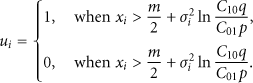
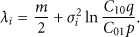
and then, with (6) and (10), the decision rule of the ith sensor can be formulated as

$u_i=\{\begin{array}{c}1,\hspace{1em}\text{when}\mathrm{\hspace{0.17em}\hspace{0.17em}}{x}_i>\frac{m}{2}+{\sigma }_i^2\ln \frac{C_{10}q}{C_{01}p},\hfill \\ 0,\hspace{1em}\text{when}\mathrm{\hspace{0.17em}\hspace{0.17em}}{x}_i>\frac{m}{2}+{\sigma }_i^2\ln \frac{C_{10}q}{C_{01}p}.\hfill \end{array}$

(11)

According to (11), the threshold of the ith sensor is

$\begin{array}{c}{\lambda }_i=\frac{m}{2}+{\sigma }_i^2\ln \frac{C_{10}q}{C_{01}p}.\end{array}$

(12)

From (12), we can see that the threshold of each sensor is different owing to the different ${\sigma }_i$ which represents the noise character of a sensor. Accordingly, taking advantage of (10), (12), and (13), the local error probabilities ${\alpha }_i$ and ${\beta }_i$ can be obtained as follows:

$\begin{array}{c}{\alpha }_i=P\left(u_i=1\hspace{0.17em}|\hspace{0.17em}{H}_0\right)={{\displaystyle \int }}_{{\lambda }_i}^{\infty }p\left(z_i\hspace{0.17em}|\hspace{0.17em}{H}_0\right)d{z}_i,\\ {\beta }_i=P\left(u_i=0\hspace{0.17em}|\hspace{0.17em}{H}_1\right)={{\displaystyle \int }}_0^{{\lambda }_i}p\left(z_i\hspace{0.17em}|\hspace{0.17em}{H}_1\right)d{z}_i.\end{array}$

(13)

3.2. Our Linear Decision Fusion Rule

In this paper, we design a novel decision fusion model and in this model, a linear equation is used to denote the integrated contribution of all the local decisions as

$\begin{array}{c}{z}_g={\displaystyle \sum }_{i=1}^n{k}_i{u}_i,\end{array}$

(14)

where $u_i$ is the local decision of the ith sensor and $k_i$ is the corresponding weight which is able to indicate the ith sensor decision-making capability. In order to understand this model better, we take a group of workers who are working together to check an event for example. Firstly, all the workers are required to try their best to draw a conclusion for this event, and then they send their decision to their leader. The leader makes a final decision depending on all the conclusions given by the workers. During this decision-making process, the decisions made by the more capable workers would be paid more attention by the leader. In this example, the workers correspond to the sensors in the mobile sensor networks, the leader corresponds to the fusion center, and the ability of the workers corresponds to the weight $k_i$ . When a sensor decision-making capability is better, its weight could be greater. In other words, if a sensor can make a decision more accurately, its contribution to $z_g$ is considered to be bigger, so it is reasonable to use $z_g={\sum }_{i=1}^n{k}_i{u}_i$ to denote the integrated contribution of local decisions in the fusion center. Then, $z_g$ would be compared with a threshold ${\lambda }_g$ , and the final decision can be made according to the following inequality expression:

$u_g=\{\begin{array}{c}1,\hspace{1em}\text{when}\mathrm{\hspace{0.17em}\hspace{0.17em}}{z}_g>{\lambda }_g,\hfill \\ 0,\hspace{1em}\text{when}\mathrm{\hspace{0.17em}\hspace{0.17em}}{z}_g<{\lambda }_g.\hfill \end{array}$

(15)

Suppose all the local decisions are independent of each other; then we can get $(P(u_1{u}_2\cdots u_n\hspace{0.17em}|\hspace{0.17em}{H}_0)={\prod }_{i=1}^{n}P(u_i\hspace{0.17em}|\hspace{0.17em}{H}_0)$ and $(P(u_1{u}_2\cdots u_n\hspace{0.17em}|\hspace{0.17em}{H}_1)={\prod }_{i=1}^{n}P(u_i\hspace{0.17em}|\hspace{0.17em}{H}_1)$ . Besides, the error probabilities ${\alpha }_g$ and ${\beta }_g$ take all the combinations of the local decisions (i.e., $u_1{u}_2\cdots u_n=00\cdots 0~11\cdots 1$ ) into account. Therefore, the two kinds of errors that the fusion center may make can be formulated as follows:

$\begin{array}{cc}\hfill & {\alpha }_g={\displaystyle \sum }_{u_1{u}_2\cdots u_n=00\cdots 0}^{11\cdots 1}{P}_{u_1{u}_2\cdots u_n}\left(u_g=1\hspace{0.17em}|\hspace{0.17em}{H}_0\right)\hfill \\ \hfill & \hspace{1em}={\displaystyle \sum }_{u_1{u}_2\cdots u_n=00\cdots 0}^{11\cdots 1}{P}_{u_1{u}_2\cdots u_n}\left({\displaystyle \sum }_{i=1}^n{k}_i{u}_i>{\lambda }_g\hspace{0.17em}|\hspace{0.17em}{H}_0\right)\hfill \\ \hfill & \hspace{1em}={\displaystyle \sum }_{u_1{u}_2\cdots u_n=00\cdots 0}^{11\cdots 1}(\phantom{\left({\displaystyle \sum }_{i=1}^n{k}_i{u}_i>{\lambda }_g\right)}P\left(u_1{u}_2\cdots u_n\hspace{0.17em}|\hspace{0.17em}{H}_0\right)\hfill \\ \hfill & \hspace{1em}\hspace{1em}\hspace{1em}\hspace{1em}\hspace{1em}\hspace{1em}\hspace{1em}\hspace{1em}\hspace{1em}\times P\left({\displaystyle \sum }_{i=1}^n{k}_i{u}_i>{\lambda }_g\right))\hfill \\ \hfill & \hspace{1em}={\displaystyle \sum }_{u_1{u}_2\cdots u_n=00\cdots 0}^{11\cdots 1}\left({\displaystyle \prod }_{i=1}^{n}P\left(u_i\hspace{0.17em}|\hspace{0.17em}{H}_0\right)\times P\left({\displaystyle \sum }_{i=1}^n{k}_i{u}_i>{\lambda }_g\right)\right),\hfill \\ \hfill & {\beta }_g={\displaystyle \sum }_{u_1{u}_2\cdots u_n=00\cdots 0}^{11\cdots 1}{P}_{u_1{u}_2\cdots u_n}\left(u_g=0\hspace{0.17em}|\hspace{0.17em}{H}_1\right)\hfill \\ \hfill & \hspace{1em}={\displaystyle \sum }_{u_1{u}_2\cdots u_n=00\cdots 0}^{11\cdots 1}{P}_{u_1{u}_2\cdots u_n}\left({\displaystyle \sum }_{i=1}^n{k}_i{u}_i<{\lambda }_g\hspace{0.17em}|\hspace{0.17em}{H}_1\right)\hfill \\ \hfill & \hspace{1em}={\displaystyle \sum }_{u_1{u}_2\cdots u_n=00\cdots 0}^{11\cdots 1}(\phantom{\left({\displaystyle \sum }_{i=1}^n{k}_i{u}_i<{\lambda }_g\right)}P\left(u_1{u}_2\cdots u_n\hspace{0.17em}|\hspace{0.17em}{H}_1\right)\hfill \\ \hfill & \hspace{1em}\hspace{1em}\hspace{1em}\hspace{1em}\hspace{1em}\hspace{1em}\hspace{1em}\hspace{1em}\hspace{1em}\times P\left({\displaystyle \sum }_{i=1}^n{k}_i{u}_i<{\lambda }_g\right))\hfill \\ \hfill & \hspace{1em}={\displaystyle \sum }_{u_1{u}_2\cdots u_n=00\cdots 0}^{11\cdots 1}\left({\displaystyle \prod }_{i=1}^{n}P\left(u_i\hspace{0.17em}|\hspace{0.17em}{H}_1\right)\times P\left({\displaystyle \sum }_{i=1}^n{k}_i{u}_i<{\lambda }_g\right)\right),\hfill \end{array}$

(16)

where

$\begin{array}{cc}\hfill & P\left(u_i=0\hspace{0.17em}|\hspace{0.17em}{H}_0\right)=q-{\alpha }_i,\hfill \\ \hfill & P\left(u_i=1\hspace{0.17em}|\hspace{0.17em}{H}_0\right)={\alpha }_i,\hfill \\ \hfill & P\left(u_i=0\hspace{0.17em}|\hspace{0.17em}{H}_1\right)={\beta }_i,\hfill \\ \hfill & P\left(u_i=1\hspace{0.17em}|\hspace{0.17em}{H}_1\right)=p-{\beta }_i.\hfill \end{array}$

(17)

According to (13), (16), and (17), the total error cost can be calculated as

$\begin{array}{c}R=\frac{C_{10}q}{C_{01}p}{\alpha }_g+{\beta }_g.\end{array}$

(18)

In order to understand this model better, we take the situation $n=2$ for example. Suppose there are only two sensors in the network and their local decisions are $u_1$ and $u_2$ , respectively. Then according to the linear decision fusion model, the integrated contribution of the two local decisions can be figured out as $z_g=k_1{u}_1+k_2{u}_2$ .

It is obvious that there are four combinations of $u_1$ , $u_2$ , and $z_g$ , as shown in Table 1.

Table 1

The combinations of $u_1$ , $u_2$ , and $z_g$ .

$u_2$	$u_1$	$z_g$
0	0	0
0	1	$k_1$
1	0	$k_2$
1	1	$k_1+k_2$

Then referring to expression (16), we can have

$\begin{array}{cc}\hfill & {\alpha }_g=P\left(u_g=1\hspace{0.17em}|\hspace{0.17em}{H}_0\right)\hfill \\ \hfill & \hspace{1em}=P\left(u_1=0\hspace{0.17em}|\hspace{0.17em}{H}_0\right)P\left(u_2=0\hspace{0.17em}|\hspace{0.17em}{H}_0\right)P\left(0>{\lambda }_g\right)\hfill \\ \hfill & \hspace{1em}\hspace{1em}+P\left(u_1=1\hspace{0.17em}|\hspace{0.17em}{H}_0\right)P\left(u_2=0\hspace{0.17em}|\hspace{0.17em}{H}_0\right)P\left(k_1>{\lambda }_g\right)\hfill \\ \hfill & \hspace{1em}\hspace{1em}+P\left(u_1=0\hspace{0.17em}|\hspace{0.17em}{H}_0\right)P\left(u_2=1\hspace{0.17em}|\hspace{0.17em}{H}_0\right)P\left(k_2>{\lambda }_g\right)\hfill \\ \hfill & \hspace{1em}\hspace{1em}+P\left(u_1=1\hspace{0.17em}|\hspace{0.17em}{H}_0\right)P\left(u_2=1\hspace{0.17em}|\hspace{0.17em}{H}_0\right)P\left(k_1+k_2>{\lambda }_g\right),\hfill \\ \hfill & P\left(u_1=0\hspace{0.17em}|\hspace{0.17em}{H}_0\right)=q-{\alpha }_1,\hfill \\ \hfill & P\left(u_1=1\hspace{0.17em}|\hspace{0.17em}{H}_0\right)={\alpha }_1,\hfill \\ \hfill & P\left(u_2=0\hspace{0.17em}|\hspace{0.17em}{H}_0\right)=q-{\alpha }_2,\hfill \\ \hfill & P\left(u_2=1\hspace{0.17em}|\hspace{0.17em}{H}_0\right)={\alpha }_2,\hfill \\ \hfill & {\beta }_g=P\left(u_g=0\hspace{0.17em}|\hspace{0.17em}{H}_1\right)\hfill \\ \hfill & \hspace{1em}=P\left(u_1=0\hspace{0.17em}|\hspace{0.17em}{H}_1\right)P\left(u_2=0\hspace{0.17em}|\hspace{0.17em}{H}_1\right)P\left(0<{\lambda }_g\right)\hfill \\ \hfill & \hspace{1em}\hspace{1em}+P\left(u_1=1\hspace{0.17em}|\hspace{0.17em}{H}_1\right)P\left(u_2=0\hspace{0.17em}|\hspace{0.17em}{H}_1\right)P\left(k_1<{\lambda }_g\right)\hfill \\ \hfill & \hspace{1em}\hspace{1em}+P\left(u_1=0\hspace{0.17em}|\hspace{0.17em}{H}_1\right)P\left(u_2=1\hspace{0.17em}|\hspace{0.17em}{H}_1\right)P\left(k_2<{\lambda }_g\right)\hfill \\ \hfill & \hspace{1em}\hspace{1em}+P\left(u_1=1\hspace{0.17em}|\hspace{0.17em}{H}_1\right)P\left(u_2=1\hspace{0.17em}|\hspace{0.17em}{H}_1\right)P\left(k_1+k_2<{\lambda }_g\right),\hfill \\ \hfill & P\left(u_1=0\hspace{0.17em}|\hspace{0.17em}{H}_1\right)={\beta }_1,\hfill \\ \hfill & P\left(u_1=1\hspace{0.17em}|\hspace{0.17em}{H}_1\right)=p-{\beta }_1,\hfill \\ \hfill & P\left(u_2=0\hspace{0.17em}|\hspace{0.17em}{H}_1\right)={\beta }_2,\hfill \\ \hfill & P\left(u_2=1\hspace{0.17em}|\hspace{0.17em}{H}_1\right)=p-{\beta }_2,\hfill \end{array}$

(19)

and then we can achieve

$\begin{array}{c}R=\frac{C_{10}q}{C_{01}p}{\alpha }_g+{\beta }_g.\end{array}$

(20)

Here, it can be seen that the value of the total error probability R depends upon $k_1$ , $k_2$ , and ${\lambda }_g$ , so if the optimal $k_1$ , $k_2$ , and ${\lambda }_g$ can be found, the smallest error probability R can be achieved. In the following content, let us discuss how to get the optimal weights $k_i$ and threshold ${\lambda }_g$ with the help of constrained PSO.

3.3. Using Constrained PSO to Control the Linear Decision Fusion Rule

It is obvious that if all the local decisions are $H_1$ ( $u_i=1,i=\mathrm{1,2},\dots ,n$ ), the final decision must be $H_1$ ( $z_g=1$ ), so we can consider that ${\sum }_{i=1}^n{k}_i=1\mathrm{\hspace{0.17em}\hspace{0.17em}}(k_i\ge 0)$ , and then, it becomes a constrained PSO problem which can be denoted as follows:

$\begin{array}{c}R=\frac{C_{10}q}{C_{01}p}{\alpha }_g+{\beta }_g,\\ {\displaystyle \sum }_{i=1}^n{k}_i=1\hspace{1em}\left(k_i\ge 0\right).\end{array}$

(21)

Here, $R=(C_{10}q/C_{01}p){\alpha }_g+{\beta }_g$ is the initial objective function and ${\sum }_{i=1}^n{k}_i=1\mathrm{\hspace{0.17em}\hspace{0.17em}}(k_i\ge 0)$ is the linear constraint. The penalty function approach is used to solve this problem. According to formulation (3) the penalty function can be established as

$\begin{array}{c}{R}^{\prime }=\frac{C_{10}q}{C_{01}p}{\alpha }_g+{\beta }_g+M{\left({\displaystyle \sum }_{i=1}^n{k}_i-1\right)}^2,\end{array}$

(22)

where M is the fixed penalty value and $({\sum }_{i=1}^n{k}_i-1{)}^2$ is the penalty factor. Then we should try to find out the smallest ${\text{R}}^{\prime }$ taking advantage of the basic PSO.

Basing on the analysis above, we can map from the basic PSO to the linear decision fusion rule, as shown in Table 2.

Table 2

PSO terminology and corresponding parameters of linear decision fusion rule.

PSO terminology	Linear decision fusion rule
Location	$(k_1,k_2,\dots ,k_n,{\lambda }_g)$
Fitness	$R^{\prime }=(C_{10}q/C_{01}p){\alpha }_g+{\beta }_g+M({{\displaystyle \sum }}_{i=1}^n{k}_i-1{)}^2\mathrm{\hspace{0.17em}\hspace{0.17em}}(k_i\ge 0)$
$p_{\text{best}}$	The location in parameter space of the smallest ${\text{R}}^{\prime }$ returned for a specific particle
$g_{\text{best}}$	The location in parameter space of the smallest ${\text{R}}^{\prime }$ returned in the entire swarm
$V_{\max \hspace{0.17em}}$	The maximum allowed velocity range in a given direction $[\mathrm{0,1}]$
$X_{\max \hspace{0.17em}}$	The maximum allowed range in a given direction $[\mathrm{0,1}]$

After that, the PSO is carried out as follows.

• (1)

Firstly, the locations of all the particles are initialized and the current location is considered as $p_{\text{best}}$ .

(2)

Secondly, the velocity and the location of each node are updated in accordance with expressions (1) and (3).

(3)

Thirdly, the new fitness is computed and the new $p_{\text{best}}$ and $g_{\text{best}}$ are generated.

(4)

Finally, if the number of iterations increases to $T_{\max \hspace{0.17em}}$ , then stop; otherwise, proceed back to step two. In this way, the optimal $(k_1,k_2,\dots ,k_n,{\lambda }_g)$ is discovered and $g_{\text{best}}$ is the smallest $R^{\prime }$ . Therefore, the smallest total error probability can be computed as $R=R^{\prime }-M({\sum }_{i=1}^n{k}_i-1{)}^2$ .

4. Performance Evaluation

In this section, we would like to demonstrate the performance of our decision fusion rule. On the platform Matlab, the basic PSO algorithm is realized and the objective function is set as $R^{\prime }=(C_{10}q/C_{01}p){\alpha }_g+{\beta }_g+M({\sum }_{i=1}^n{k}_i-1{)}^2$ . In order to obtain the smallest $R^{\prime }$ , a swarm consists of 25 particles flying around in an $(n+1)$ -dimensional search space, where n is the number of network sensors. In the end of searching process, the $g_{\text{best}}$ should be the smallest $R^{\prime }$ , and then, with $R^{\prime }$ , the smallest error probability R for our fusion rule can be obtained. Consequently, the corresponding $k_i$ and ${\lambda }_g$ are the optimal parameters of the fusion rule.

Firstly, whether the parameters of PSO can affect the performance of our decision fusion rule is demonstrated in Section 4.1. Then, in Section 4.2, let us show that what would happen to our experimental results as the number of sensors increases.

4.1. Choosing PSO Parameters w, $c_1$ , and $c_2$

It can be seen from expression (1) that the optimal performance of PSO depends on the values of parameters w, $c_1$ , and $c_2$ . The inertia parameter w controls the momentum of each particle. A larger w can increase the global exploration ability while a smaller w tends to improve the local exploration ability of particles. The cognitive learning parameter $c_1$ limits the contribution of a specific particle $p_{\text{best}}$ while the social learning parameter $c_2$ limits the contribution of the entire swarm $g_{\text{best}}$ .

At first, let us discuss the performance of our fusion rule when inertia parameter w is fixed or changes along with time. In the first case, we set $w=0.5$ while, in the second case, we set $w=w_{\max \hspace{0.17em}}-((w_{\max \hspace{0.17em}}-w_{\min \hspace{0.17em}})/T_{\max \hspace{0.17em}})\times t$ , where t and $T_{\max \hspace{0.17em}}$ are, respectively, the current and maximum number of iterations and $w_{\max \hspace{0.17em}}$ and $w_{\min \hspace{0.17em}}$ are, respectively, the upper and lower bounds of w. In this paper, we set $w_{\max \hspace{0.17em}}=0.9$ , $w_{\min \hspace{0.17em}}=0.4$ , and $T_{\max \hspace{0.17em}}=1500$ . The inputs and outputs of this simulation are as shown in Table 3.

Table 3

The simulation results with different inertia parameter w when the sensor number is 10.

Inputs $(c_1=c_2=2)$	Outputs
Inertia parameter w	Total error probability R	Time consumed for convergence (iterations)
$w=0.5$	0.00181079	447
$w=w_{\max \hspace{0.17em}}-((w_{\max \hspace{0.17em}}-w_{\min \hspace{0.17em}})/T_{\max \hspace{0.17em}})\times t=0.9-(0.5/1500)\times \text{t}$	0.00120768	123

From Table 3 and Figure 3, we can see that when the inertia parameter w changes along with time, the total error probability R is lower and the time consumed for convergence is shorter than those when w is fixed. The reason is that if we choose the time-variable inertia parameter, particles can have good global exploration ability at the beginning phase of the searching process and good local exploration ability as the current number of iterations increases. Thereby, we decide to choose the time-variable inertia parameter w.

Figure 3

The simulation results with time-variable and fixed inertia parameter w.

After that, let us discuss the learning parameters $c_1$ and $c_2$ . If $c_1=0$ or $c_2=0$ , it means that we do not take the cognitive learning process or the society learning process into account. Under this situation, the simulation results are as shown in Table 4.

Table 4

The simulation results with different learning parameters $c_1$ and $c_2$ when the sensor number is 10.

Inputs $(w=w_{\max \hspace{0.17em}}-((w_{\max \hspace{0.17em}}-w_{\min \hspace{0.17em}})/T_{\max \hspace{0.17em}})\times t)$	Outputs
$c_1$ and $c_2$	Total error probability R	The number of iteration
$c_1=c_2=2$	0.00120768	123
$c_1=0,c_2=2$	0.00274277	150
$c_1=2,c_2=0$	0.00121506	Cannot converge

From Table 4 and Figure 4, it can be seen that when the cognitive learning parameter $c_1$ is not taken into account, PSO still can get converged, but the total error probability R becomes larger and time consumed for convergence is longer comparing with the situation when $c_1\ne 0$ . When we do not consider the society learning parameter $c_2$ , PSO cannot get converged at all. The reason is that each particle only has the knowledge about itself, so the swarm can never evolve to the same direction.

Figure 4

The experimental results with different learning parameters.

In sum, from the analysis above, we can see that the time-variable inertia parameter w is better than the fixed one and the situation that both learning parameters $c_1$ and $c_2$ are taken into account is better than the situation when $c_1=0$ or $c_2=0$ . Therefore, in the following simulation, the parameters are set as

$\begin{array}{c}w=w_{\max }-\frac{w_{\max }-w_{\min }}{T_{\max }}\times t,\\ c_1=c_2=2.\end{array}$

(23)

4.2. The Performance of Linear Fusion Rule with Different Sensor Numbers

Here, the number of sensors in the network is set as $n=5$ , $n=10$ and $n=15$ , respectively. According to the experimental results, it can be seen that our decision fusion rule can indeed get very high accuracy. The inputs and outputs of our simulation are as shown in Table 5 and Figure 5.

Table 5

The inputs and outputs of the simulation.

Inputs ( $\text{mean}=0$ , $M=10$ , $P=0.8$ , $q=0.2$ )		Outputs
n	Differences	$(k_1,k_2,\dots ,k_n)$	${\lambda }_g$	$R=R^{\prime }-M({\sum }_{i=1}^n{k}_i-m{)}^2{k}_i$
5	(43.86, 52.63, 26.2, 39.39, 80.08)	(0.102567, 0.463625, 0.0806701, 0.019778, 0.333359)	0.704058	0.0342967
10	(43.86, 52.63, 26.2, 39.39, 80.08, 47.16, 45.09, 34.65, 67.89, 54.78)	(0.191843, 0.253623, 0.0650721, 0.00822591, 0, 0.158283, 0.0213777, 0.251185, 0.00907494, 0.0413086)	0.745094	0.00116502
15	(43.86, 52.63, 26.2, 39.39, 80.08, 47.16, 45.09, 34.65, 67.89, 54.78, 34.76, 56.34, 27.89, 47.89, 38.97)	(0.0244901, 0.157784, 0.368528, 0.10523, 0.0614695, 0.0173535, 0.0114619, 0, 0.00495967, 0.048092, 0.00231704, 0, 0.0210975, 0.127067, 0.0500054)	0.334601	0.0000403

Figure 5

The experimental results under different sensor numbers n.

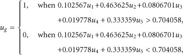
When $n=5$ , the decision fusion rule becomes

$\begin{array}{c}{u}_g=\{\begin{array}{c}1,\hspace{1em}\text{when}\mathrm{\hspace{0.17em}\hspace{0.17em}}0.102567u_1+0.463625u_2+0.0806701u_3\hfill \\ \hspace{1em}\hspace{1em}\hspace{1em}\hspace{1em}\mathrm{\hspace{0.17em}\hspace{0.17em}}+0.019778u_4+0.333359u_5>0.704058,\hfill \\ 0,\hspace{1em}\text{when}\mathrm{\hspace{0.17em}\hspace{0.17em}}0.102567u_1+0.463625u_2+0.0806701u_3\hfill \\ \hspace{1em}\hspace{1em}\hspace{1em}\hspace{1em}\mathrm{\hspace{0.17em}\hspace{0.17em}}+0.019778u_4+0.333359u_5<0.704058,\hfill \end{array}\end{array}$

(24)

and, with these parameters, we can get the total error probability $R=0.0342967$ which is very small. After about more than 50 iterations, the PSO has already got converged, so the time consumed is very short.

Similarly, from Table 5 and Figure 5(b), when $n=10$ , we can see that the total error probability becomes $R=0.00116502$ and after about 120 iterations the PSO gets converged. When $n=15$ , $R=0.0000403$ which is close to zero and after 150 iterations the PSO gets converged.

As shown in Figure 6, along with the increase of n, the error cost becomes smaller and smaller. This phenomenon is easy to understand because the decision result is more precise when there are more sensors working in the network. However, as n increases, the time consumed for PSO to find the optimized parameters becomes longer, so when this fusion rule is used we should better get a balance between accuracy and time.

Figure 6

The total error probability R and time consumed for convergence change along with sensor number.

In brief, this simulation indicates that our linear fusion rule is capable of getting really small total error probability under the control of the constrained PSO, also showing that PSO does very well for the parameter optimization of the linear decision fusion rule.

5. Conclusion

In this paper, we present a linear decision fusion model and propose a way of controlling the parameters of the model taking the advantage of the constrained PSO. In the model, the integrated contribution of local decisions is computed with a linear equation which is made up with local decision weights and local decisions, and then the integrated contribution is compared with a threshold in the fusion center. After that, according to the comparison results, the final decision can be made. Furthermore, the constrained PSO is creatively employed to discover the weights and the threshold. The simulation results show that our linear decision rule and the way of parameter optimization are efficient to get very high accuracy.