On Guaranteed Detectability for Surveillance Sensor Networks

Abstract

Surveillance is an important class of applications for wireless senor networks (WSNs), whose central task is to detect events of interest. Existing approaches seriously suffer from blind spots and low energy efficiency. In this paper, we propose a fully distributed algorithm GAP for energy-efficient event detection for surveillance applications. Employing the probabilistic approach, GAP actively tunes the active probability and minimizes the energy consumption of each sensor. The unique features of GAP are threefold. First, it provides guaranteed detectability for any event occurring in the sensing field. Second, it exposes a convenient interface of the user to specify the desired detectability. Finally, it supports differentiated service to empower better surveillance for critical spots. Without relying on costly time synchronization, GAP is a lightweight distributed protocol and is truly scalable to network scale and sensor density. Theoretical analysis and comprehensive simulation experiments are conducted, which jointly demonstrate that GAP is able to provide guaranteed detectability while significantly prolonging the system lifetime compared with other schemes.

1. Introduction

Recent rapid advances in wireless sensor networks (WSNs) have made it possible to develop a wide multitude of compelling applications, ranging from battlefield surveillance, habitat monitoring, and radiation prevention [1] to pollution detection [2]. Surveillance, whose central task is to detect events of interest, is an important class of applications for WSNs. The most important performance goal for surveillance applications is high detectability. Among the others, fire detection in large-scale forest is a good example of surveillance applications.

It is well known that tiny sensor nodes are subject to stringent energy constraint since they are powered by small batteries. This implies that a sensor node has only a short lifetime. It is usually impractical, if not impossible, to recharge or replace batteries after sensor nodes are deployed to a remote or event hostile environment. However, applications require the network to sustain surveillance operations for a long lifetime. It has been challenging to obtain a long-lived network with tiny short-lived sensor nodes. To achieve high detectability, the straightforward way is to keep all sensors active such that an event is sure to be detected. However, it is obvious that this scheme suffers from low energy efficiency, especially when sensor density is high. In this paper, we focus on energy-efficient surveillance using networked sensors.

The fundamental approach to conserving energy is to power off sensors. Many research efforts have been made for energy-efficient surveillance using sensor networks. In general, they select a subset of sensor nodes to keep vigilant for event detection and put the others in power-save mode. In PEAS [3], a sensor probes neighbors to check if there are active neighbors. Upon receiving acknowledgement from an active neighbor, it goes to sleep. Network provisioning [4] identifies a redundant sensor whose sensing coverage is jointly covered by its active neighbors. Yan et al. [5] noted the underestimation problem that exists in [4] and proposed a randomized algorithm to determine an active schedule of the sensors.

There are two major drawbacks with the existing methods. First, the algorithms’ failing to provide full coverage over the sensing field suffers from blind spots that are not covered by any active sensors. Events occurring in these blind spots will not be detected, leading to serious surveillance quality degradation. Second, the algorithms suffer from the critical problem of unbalanced energy consumption. According to the existing algorithms, a set of sensors are selected to stay active for full sensing coverage while the other sensors turn to power-save mode. The consequence is that the selected active sensors will be depleted earlier. If an active sensor becomes unavailable due to power depletion or physical damage, the area covered by this sensor will become a blind spot.

In addition to identifying the limitations of existing approaches, we have two important observations for many realistic surveillance applications.

• (i)

It is unnecessary for many applications, such as habitat monitoring, to have perfect detectability (i.e., 100% detectability). For example, a wild animal of interest may cause a number of events in the field. It is sufficient for the animal study to capture some of the events. In practice, different applications usually have varying requirements on detectability. It is clear that more sensitive applications are usually in need of higher detectability.

(ii)

An event can occur at any unpredictable time at any place within the sensing field. It is impossible to predict the location where the next potential event occurs.

In response to the two observations, the system design should satisfy two important requirements for such surveillance applications.

• (i)

The system should allow the users to customize the desirable detectability, given different applications.

(ii)

The system should guarantee that the detectability of any event occurring in the sensing field is larger than the requirement posed by the user.

To the best of our knowledge, no existing algorithms can successfully satisfy the requirements mentioned above. In this paper, we propose a novel-distributed algorithm GAP to provide guaranteed detectability for any event in the whole sensing field. The algorithm exposes a convenient interference for the users to specify the desirable minimum detectability. We devise a simple yet effective metric to realize the design goal of providing guaranteed detectability of any potential event. Exploiting the probabilistic approach, the algorithm allows the sensors to be active probabilistically for effective energy conservation. The algorithm actively minimizes the active probability of each sensor, which is also adaptive to its neighborhood of sensor deployment. Energy consumption of the sensors is finely balanced. At the same time; however, the detectability of any event in the sensing field is dynamically maintained.

The contributions we have made in this paper are highlighted as follows.

• (1)

We develop the fully distributed GAP algorithm that can provide guaranteed detectability for any event. Not relying on costly time synchronization, this algorithm is lightweight and fully distributed, supporting truly scalability with network scale and sensor density.

(2)

The GAP algorithm empowers differentiated surveillance in terms of detectability and detection degree, which greatly enhances its practical applicability.

(3)

We conduct both theoretical analysis and comprehensive simulations to validate the design and study the performance of the GAP algorithm.

The remainder of the paper is structured as follows. In Section 2, we discuss related work. In Section 3, we introduce the system model and some preliminaries. In Section 4, after detailing the GAP design, we discuss several design issues and present algorithm analysis. To study the performance of GAP, we conduct comprehensive experiments and discuss the results in Section 5. In Section 6, we give some discussions about the algorithm design. Finally, we conclude the paper and introduce future work.

2. Related Work

In this section we review related work and discuss the difference of our work from existing studies.

2.1. Duty Cycling in Sensor Networks

It has been the subject of extensive research to conserve energy in WSNs through power management or duty cycling. With duty cycling, a sensor node periodically enters power-saving mode for energy saving and wakes up for sensing and communication tasks. Three power-saving protocols for mobile ad hoc networks were developed in [4], which provide different tradeoffs between energy efficiency and neighbor discovery latency. Without relying on time synchronization, asynchronous wakeup [6] is advantageous. However, it comes with the cost of increased packet delivery latency. Different tradeoffs between packet delivery latency and energy saving were studied in [7].

Low duty cycling has been recognized as an effective technique to realize operation longevity in sensor networks. In [8], the scheduling problem of multiple tasks in low-duty-cycled sensor networks is studied. In [9], the energy fairness of asynchronous duty cycling sensor networks is explored. Our work in this paper also adopts duty cycling for every saving but has a focus on the determination of duty cycles for each sensor node making sure that the event detection of any possible event is guaranteed.

2.2. Power Management of Sensor Networks

With power management, a subset of sensor nodes are selected for sensing or communication purposes. In surveillance applications, a number of algorithms were proposed to select a subset of sensor nodes to stay vigilant for event detection while the others remain in power save mode. PEAS [3] selects active sensors by active probing. Each sensor probes its neighborhood. If there is an active sensor responding its probing, the sensor decides to sleep; otherwise, it stays active. PEAS does not providing full sensing coverage and therefore suffers from the blind spot problem. Network-provisioning [10] identifies a sensor to be in sleep mode if sensing coverage of this sensor is jointly covered by its active neighbors. Several efforts, for example, the one in [11], take both sensing coverage and network connectivity into account. These algorithms provide full sensing coverage and meanwhile maintain network connectivity.

Tian and Georgana [4] noted the underestimation problem that exists in [4] and proposed a randomized algorithm to determine an active schedule of each sensor. According to this algorithm, each sensor is activated for event detection periodically. Thus, this algorithm solves, to some extent, the problem of unbalanced energy consumption. A probabilistic approach has been proposed for event detection in the context of object tracking [2], which can also mitigate the problem of unbalanced energy consumption. However, these algorithms cannot provide guaranteed detectability for the sensing field.

Shih et al. [12] propose to use a small-scale sensor network to monitor epilepsy. It is reported that 21 scalp electrodes are needed and 18 data streams or channels are generated. In order to save the energy consumption of the data processing device that is battery powered and attached to a user, they propose an automated way to construct detectors that use fewer channels, and thus fewer electrodes.

2.3. Energy-Efficient Event Detection

As is widely known, event detection [13] is an important class of applications of sensor networks. Exploiting the inherent property of event persistence, some algorithms [14, 15] try to detect events with low duty-cycled sensor networks. In [16], a two-stage optimization was proposed to minimize detection latency. In the first stage, a density control algorithm is applied to select a set of active nodes. In the second stage, an optimization procedure is executed to schedule wakeups of the sensors, which relies on accurate location information. A testbed of 70 sensors was deployed to detect and track the positions of moving vehicles [17]. In this system, 5% of deployed motes serve as sentries and nonsentries operate at a 4% duty cycle. An improved system with a combination of duty cycle scheduling, sentry service, and tripwire service was recently reported in [18]. With low duty cycling, the lifetime of the system can be significantly extended by up to 900%.

Different from these existing studies, our paper specially considers the guarantee of event detection performance while conserving energy consumption on sensor nodes.

2.4. Energy Harvesting in Sensor Networks

Recently, energy harvesting techniques are becoming very promising technology for long-term applications of sensor networks. In [19], Gu et al. point out that it is unnecessary to conserve energy in sensor networks with energy harvest ability, and instead it is more important to balance energy supply and energy consumption. They propose a middleware to control the RF activity with the objective of minimizing communication delay.

Zhu et al. [20] notice the leakage problem of energy capacitors. They propose leakage-aware feedback control techniques to match local and network-wide activity of sensor nodes that obtain dynamic energy supply from environments.

In [21], a system called eShare is described to support energy sharing among multiple-embedded sensor devices. They design energy routers for energy storage and routing devices. Energy access and network protocols are also designed. To improve sharing efficiency subject to energy leakage, an energy charging and discharging mechanism is devised.

The preliminary result of this research has previously been reported in [15] and in this paper we consolidate the research with investigation on design issues, algorithm analysis, and discussions.

3. System Model and Preliminaries

In this section, we first describe the system model and formally state the problem. Second, we define the necessary notations and make several simplifying assumptions. Third, we devise a metric that helps realize the effective guarantee of required detectability for any event. Finally, we analyze the detectability of the nonadaptive scheme in which sensors stay active blindly, and reveal the necessity of adaptive control on sensor active probability.

3.1. System Model and Problem Statement

We consider the sensors are deployed in a square field F with side length L according to a 2-dimensional Poisson process with rate $n/L^2$ . Under this deployment, the number of sensors in any given region of area A is Poisson distributed with rate $nA/L^2$ . The number of sensors in disjoint regions is independent. Usually, a random uniform distribution of points over a region can be approximated by a 2-dimensional Poisson process. Note that the actual number of nodes deployed in the field needs not to be n. A random uniform deployment can be approximated by a 2-dimensional Poisson deployment when the number of deployed sensors is sufficiently large.

The power consumption of a sensor node lies in three major units: processor, sensing device, and radio transceiver. Ideally, each unit has separate power control [10]. The duty cycle of the transceiver is subject to the control of communication protocols. Therefore, we assume it is given and concentrate on the study of duty cycling of the sensing device. The transceiver does not necessarily has the same duty cycle as the sensing device. The consequent advantage is the increased flexibility for our protocol to work with different communication protocols. It is important to note that a sensor node can actually be attached with multiple-sensing devices of different types. For simplification; however, we assume that a sensor node is equipped with a single-sensing device throughout the analysis and the protocol design. Nevertheless, the protocol can be easily extended to support the situation where a sensor node has multiple-sensing devices. Later, we call a sensor node just a sensor for short if it is not confused with the sensing device.

It should be noted that such an power model assumes that all the units can be independently controlled. In some cases, however, a sensor node may not be able to independently control the power consumption of each unit. In such cases, a sensor node has only one unit and has a single duty cycle. Our power model is general and covers such cases.

The objectives of the system design are twofold. First, users should be enabled to specify the lowest detectability (denoted by ${\upsilon }_0$ ) for any event in the sensing field. The system needs to ensure that the detectability of such a random event is greater than the required detectability. Second, event detection of the sensors should be energy-efficient such that the system can continue to be functional for a very long lifetime.

To accomplish these objectives, we have identified the key issues in the system design as follows.

• (1)

The system needs an effective way to realize the goal of providing guaranteed detectability for any possible event.

(2)

The algorithm should minimize the active probability of every sensor, thus minimizing the energy consumption of the sensor.

(3)

The power consumption of the sensors should be balanced such that as few blind spots as possible are introduced.

3.2. Notations and Assumptions

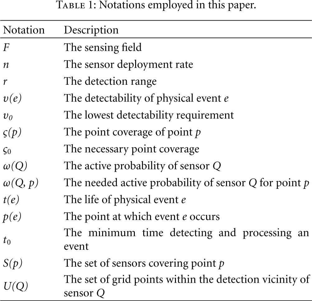
In the rest of this paper, we adopt the notations in Table 1 and make the following assumptions.

• (i)

Binary Detection Model. Each sensor has a detection range. An event is reliably detected by an active sensor if it resides in the range of an active sensor. More sophisticated models suggest that the detection probability is related to the distance between the sensor and the event. We assume that the detection range in our binary detection model is selected such that an event can be detected with high probability if its distance to the sensor is less than the detection range.

(ii)

Location Awareness. Each sensor has the knowledge of its location. A good number of power-efficient algorithms have been proposed for practical localization in large-scale WSNs [22].

(iii)

High Density. There are sufficient sensors deployed in the sensing field such that any point in the sensing field is covered by at least one sensor.

Table 1

Notations employed in this paper.

Notation	Description
F	The sensing field
n	The sensor deployment rate
r	The detection range
υ(e)	The detectability of physical event e
υ 0	The lowest detectability requirement
ς (p)	The point coverage of point p
ς 0	The necessary point coverage
ω(Q)	The active probability of sensor Q
ω(Q, p)	The needed active probability of sensor Q for point p
t(e)	The life of physical event e
p(e)	The point at which event e occurs
t 0	The minimum time detecting and processing an event
S(p)	The set of sensors covering point p
U(Q)	The set of grid points within the detection vicinity of sensor Q

In the protocol design, we assume that the sensor network is deployed in a two-dimensional plane. However, the proposed protocol can be extended to a three-dimension space without much difficulty.

3.3. Realizing Detectability Guarantee

To realize the goal of providing guaranteed detectability for any event, we devise a simple but effective metric: point coverage. Its precise definition is given as follows.

Definition 1.

For a point p within the sensing field, the point coverage of p, denoted by $\varsigma (p)$ , is defined as the probability that p is covered by at least one sensor at any time.

The point coverage of p is dependant on the number of covering sensors and the active probabilities of these sensors. Let 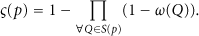$\omega (Q)$ denote by the probability that sensor Q is active at any time. It is apparent that a sensor has a longer lifetime if it has a lower active probability. In the sensing field, a point can be in the detection range of many sensors. Let $S(p)$ denote the set of sensors that cover point p. The point coverage of p is given by

$$\begin{array}{cc}& \varsigma \left(p\right)=\mathrm{1}-\prod _{\forall Q\in S\left(p\right)}\left(\mathrm{1}-\omega \left(Q\right)\right).\end{array}$$

(1)

With the concept of point coverage, we show that Objective A is implied if we achieve Objective B.

Objective A

to guarantee that the detectability of any event is larger than the minimum requirement.

Objective B

to ensure that the point coverage of any point in the field is larger than a given value.

Let $t(e)$ denote the lifetime of event e. The detectability of this event depends on both the event life and the point coverage of the location where the event resides. Let $t_0$ be the minimum necessary time required for a sensor to detect and process an event. Then, the detectability of e is given by

$$\begin{array}{cc}& \upsilon \left(e\right)=\mathrm{1}-{\left(\mathrm{1}-\varsigma \left(p\left(e\right)\right)\right)}^{t\left(e\right)/t_{\mathrm{0}}}.\end{array}$$

(2)

Event life $t(e)$ is usually a random variable. Given the probability density distribution of $t(e)$ , denoted by $f_{t(e)}$ , we can compute the expected detectability of a random event

$$\begin{array}{cc}& E\left(\upsilon \left(e\right)\right)={\int }_{t=\mathrm{0}}^{\infty }\left(\mathrm{1}-{\left(\mathrm{1}-\varsigma \left(p\left(e\right)\right)\right)}^{t/t_{\mathrm{0}}}\right)f\left(t\right)dt.\end{array}$$

(3)

It is apparent that the expected detectability monotonously increases with the increasing point coverage of $p(e)$ . To ensure that the detectability of the event is greater than the required detectability,

$$\begin{array}{cc}& E\left(\upsilon \left(e\right)\right)\ge {\upsilon }_{\mathrm{0}},\end{array}$$

(4)

we can calculate the minimum point coverage ( ${\varsigma }_0$ ) such that,

$$\begin{array}{cc}& {\int }_{t=\mathrm{0}}^{\infty }\left(\mathrm{1}-{\left(\mathrm{1}-{\varsigma }_{\mathrm{0}}\right)}^{t/t_{\mathrm{0}}}\right)f\left(t\right)dt={\upsilon }_{\mathrm{0}}.\end{array}$$

(5)

Based on the monotony of the expected detectability as a function of point coverage, we can develop a numerical procedure to obtain the desired ${\varsigma }_0$ . Let

$$\begin{array}{cc}& {\varsigma }_{\mathrm{0}}=g\left({\upsilon }_{\mathrm{0}}\right).\end{array}$$

(6)

It then becomes obvious that the expected detectability of e is guaranteed to be greater than the required ${\upsilon }_0$ as long as the point coverage of $p(e)$ is maintained above ${\varsigma }_0$ . Considering the arbitrary selection of the event, we conclude that by providing the guaranteed minimum point coverage of any point within the sensing field,

$$\begin{array}{cc}& \varsigma \left(p\right)\ge {\varsigma }_{\mathrm{0}},\hspace{1em}\forall p\in F,\end{array}$$

(7)

the system is able to ensure that the detectability of any event is greater than the required ${\upsilon }_0$ .

For pictorial study, we plot the necessary point coverage as a function of the required detectability in Figure 1. For simplification, we consider the lifetime of events as a fixed value. We can see that the necessary point coverage increases when the required detectability becomes higher. However, when the event lifetime becomes larger, the necessary point coverage can be dramatically reduced.

Figure 1

Necessary point coverage as a function of detectability requirement.

3.4. Detectability Analysis for Nonadaptive Scheme

There is a straightforward solution (called NAS) to provid guaranteed detectability to the sensing field; that is, guaranteeing that the point coverage of any point is greater than ${\varsigma }_0$ . According to this scheme, every sensor has the identical active probability of ${\varsigma }_0$ . When the deployment density is sufficiently large, it is obvious that this scheme can successfully provide the guaranteed detectability. However, this scheme does not scale as more sensors are deployed in the sense that additional sensor deployment does not result in extended system lifetime. We illustrate the problem by analyzing the actual detectability of any event achieved by NAS. Firstly, we study the point coverage as a function of number of deployed sensors.

Let point p be an arbitrary point in the field. Note that we do not consider the special case of points on the edge. The number of sensors covering p (denoted by N) is a random number. Since the sensors are deployed according to a 2-dimensional Poisson process, N has a Poison distribution. The probability mass function of N is given by

$$\begin{array}{cc}& \text{Pr}\left(N=k\right)=\frac{\mathrm{1}}{k!}{\lambda }^k{e}^{-\lambda },\hspace{1em}\text{where}\hspace{0.17em}\hspace{0.17em}\lambda =\frac{n\pi r^{\mathrm{2}}}{L^{\mathrm{2}}}.\end{array}$$

(8)

Theorem 2.

The expected point coverage of a point in the sensing field is given by

$$\begin{array}{cc}& E\left(\varsigma \left(p\right)\right)=\mathrm{1}-e^{-\lambda {\upsilon }_{\mathrm{0}}}.\end{array}$$

(9)

Proof.

Let point p be an arbitrary point in the field. The point coverage of p is given by

$$\begin{array}{cc}& \varsigma \left(p\right)=\mathrm{1}-{\left(\mathrm{1}-{\varsigma }_{\mathrm{0}}\right)}^N.\end{array}$$

(10)

The point coverage of p is actually a random variable since it relies on the number of covering sensors. We are interested in the expected $\varsigma (p)$ . We condition on N to compute this expected value,

$$\begin{array}{ll}& E\left(\varsigma \left(p\right)\right)=\sum _{i=\mathrm{1}}^n\left(\left(\mathrm{1}-{\left(\mathrm{1}-{\varsigma }_{\mathrm{0}}\right)}^i\right)\times \text{Pr}\left(N=i\right)\right)\\ =\mathrm{1}-e^{-\lambda {\varsigma }_{\mathrm{0}}}.\end{array}$$

(11)

Theorem 3.

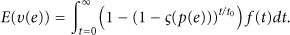
The expected detectability of any event occurring in the sensing field is given by

$$\begin{array}{ll}& E\left(\upsilon \left(e\right)\right)={\int }_{t=\mathrm{0}}^{\infty }\left(h\left(i,t\right)\cdot \text{Pr}\left(N=i\right)\right)f\left(t\right)dt,\\ \hspace{1em}\text{where}\hspace{0.17em}\hspace{0.17em}h\left(i,t\right)=\mathrm{1}-{\left(\mathrm{1}-{\varsigma }_{\mathrm{0}}\right)}^{\left(i\cdot t\right)/t_{\mathrm{0}}}.\end{array}$$

(12)

Proof.

We consider an arbitrary event e occurring point p in the sensing field. Suppose the number of sensors coving p is N and the event life of e is t. According to (10) and (2), we can obtain the detectability of e,

$$\begin{array}{cc}& \upsilon \left(e\right)=\mathrm{1}-{\left(\mathrm{1}-{\varsigma }_{\mathrm{0}}\right)}^{\left(N\cdot t\right)/t_{\mathrm{0}}}.\end{array}$$

(13)

To compute the expected detectability, we first condition on N and then consider the probability density of t. This completes the proof.

To study the expected detectability when the system parameters vary, we plot the expected detectability as a function of the number of sensor nodes. For simplification, we consider the lifetime of events as a fixed value equal to $t_0$ . We set the field side to 300 m. The detection range of the sensor is 10 m. We vary the number of sensors from 4000 to 10000. In this case, the expected detectability is given by

$$\begin{array}{cc}& E\left(\upsilon \left(e\right)\right)=\mathrm{1}-e^{-\lambda {\varsigma }_{\mathrm{0}}}.\end{array}$$

(14)

Figure 2 shows the expected detectability as a function of the number of deployed sensors under different detectability requirements. We can see that the actual detectability is dramatically larger than the required detectability even when the density of the sensors are relatively low. With the increasing number of sensors, the detectability quickly converges to one. This suggests that NAS is not scalable to the sensor density, thus wasting precious energy.

Figure 2

Expected detectability as a function of number of deployed sensors; $t(e)=t_0$

4. Design of GAP

In this section, we first give an overview of the design of GAP. Next, we describe the detailed design. Third, we discuss some design issues. Finally, we present the analysis of the algorithm.

4.1. Overview

There are two critical design goals for GAP. On one hand, it should ensure that the point coverage of any point in the sensing field is not less than ${\varsigma }_0$ . On the other hand, it needs to reduce energy consumption of every sensor, thereby extending the system lifetime as much as possible. The algorithm adopts a probabilistic approach, where every sensor probabilistically stays active. At any time, a sensor Q is active with probability of $\omega (Q)$ and is in power save mode with probability of $1-\omega (Q)$ .

The central issue of the GAP design is the determination of the active probability of each sensor. It is intuitive that the active probability should be minimized for the purpose of higher energy efficiency. However, at the same time it should be sufficiently large to ensure that point coverage of any point is above ${\varsigma }_0$ . This poses a rigid requirement on the algorithm design. To exploit the dense deployment and balance energy consumption of the sensors, GAP adaptively tunes the active probability of every sensor such that the active probability is minimized but is adequate to ensure that the lowest point coverage within its detection vicinity is not less than ${\varsigma }_0$ .

The GAP algorithm consists of two phases. In the first phase, each sensor conservatively selects an initial active probability based on the neighborhood information. The initial probability is so sufficiently large that the point coverage of any point is larger than ${\varsigma }_0$ . To solve the energy waste introduced by the conservativeness, in the second phase, each sensor executes an iterative refinement procedure to reduce active probability for better energy efficiency. The refinement procedure terminates in finite number of steps. As there are infinitely points in the sensing field, we divide the field into virtual grids, as shown in Figure 4. We consider grid points and will later show that these grid points are sufficient in providing guaranteed detectability for any point. Figure 3 depicts the state transition diagram of the proposed algorithm.

Figure 3

State transition diagram of the GAP algorithm.

Figure 4

Grid points layout for active probability determination.

4.2. Design Details

4.2.1. Neighbor Discovery

At the beginning, each sensor discovers its neighbors within 2r distance from itself by exchanging HELLO messages with each other. A HELLO message encloses the ID and the location of the sensor. For a given sensor, a neighbor is a detection neighbor (distinguished from a communication neighbor) if its distance to the neighbor is less than 2r. Every sensor maintains a table for its detection neighbors. Upon receiving a HELLO, the sensor records the sender in the table if the sender is a detection neighbor; otherwise, this packet is silently dropped. Note that such small HELLO messages can be piggybacked through other protocol packets for energy efficiency, such as localization messages in the initialization process. The time period for neighbor discovery should be sufficiently long such that each sensor can broadcast its HELLO message.

4.2.2. Initial Probability Selection

After neighbor discovery, the sensors start to compute its initial active probability. The initial active probability guarantees that the point coverage of any point in the field is greater than ${\varsigma }_0$ .

The point coverage of p is given by

$$\begin{array}{cc}& \varsigma \left(p\right)=\mathrm{1}-\prod _{B\in S\left(p\right)}\left(\mathrm{1}-\omega \left(B\right)\right).\end{array}$$

(15)

To guarantee that the point coverage is not less than ${\varsigma }_0$ , each sensor initially computes the probability needed for every single grid point within its detection vicinity, and then calculates the active probability needed at the sensor. Each sensor Q considers a grid point p and computes the active probability needed for p, denoted by $\omega (Q,p)$ . With the consideration of energy balance, we let the sensors covering p play an equally important role in detecting events at p. Thus, Q figures out the number of detection neighbors that cover p by checking the table of detection neighbors. Then Q is able to compute $\omega (Q,p)$ ,

$$\begin{array}{cc}& \omega \left(Q,p\right)=\mathrm{1}-\sqrt[k]{\mathrm{1}-{\varsigma }_{\mathrm{0}}},\hspace{1em}\text{where}\hspace{0.17em}\hspace{0.17em}k=\left|S\left(p\right)\right|\ge \mathrm{1}.\end{array}$$

(16)

To compute the initial active probability for sensor Q, it takes the maximum of the active probabilities for all grid points within its detection vicinity. Let $U(Q)$ denote the set of all the grid points within the detection range of Q. Then, the active probability of Q is

$$\begin{array}{cc}& \omega \left(Q\right)=\max \left\{\omega \left(Q,p\right),\forall p\in U\left(Q\right)\right\}.\end{array}$$

(17)

The selection of the initial probability is conservative in the sense that it takes the maximum value as its active probability to ensure that every point in its detection vicinity provides larger point coverage than required. The consequence is that the point coverage of a point may actually be much larger than the required one. Such conservativeness incurs additional energy consumption and therefore leads to less energy efficiency.

4.2.3. Refining Active Probabilities

To solve the problem introduced by the conservativeness of the initial selection, we propose a coordinated probability refinement procedure, which is a completely localized algorithm. Each sensor recalculates a new active probability based on the active probabilities of its detection neighbors. If the newly computed active probability is smaller, it tries to update its active probability, attempting to reduce its duty cycle. It is guaranteed that this refinement procedure terminates in finite number of rounds.

After determining the initial active probability, sensors exchange their active probabilities by local broadcast. Each sensor recalculates a feasible active probability based on the active probabilities of its detection neighbors. Similarly, a sensor firstly computes a new active probability for each grid point. Consider a point p. The new feasible active probability of Q for p is given by

$$\begin{array}{ll}& {\omega }^{\left(k+\mathrm{1}\right)}\left(Q,p\right)=\{\begin{array}{ll}\mathrm{1}-\frac{\mathrm{1}-{\varsigma }_{\mathrm{0}}}{y},\hfill & \text{if}\hspace{0.17em}\hspace{0.17em}\mathrm{1}-{\varsigma }_{\mathrm{0}}<y\hfill \\ \mathrm{0},\hfill & \text{otherwise},\hfill \end{array}\\ \hspace{1em}\text{where}\hspace{0.17em}\hspace{0.17em}y=\prod _{B\in S\left(p\right)-\left\{Q\right\}}\left(\mathrm{1}-{\omega }^{\left(k\right)}\left(B\right)\right),\end{array}$$

(18)

where (k) denotes the number of generations of the associating active probability.

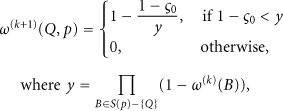
To compute the new active probability, Q also takes the maximum out of all the grid points within its detection vicinity,

$$\begin{array}{cc}& {\omega }^{\left(k+\mathrm{1}\right)}\left(Q\right)=\max \left\{{\omega }^{\left(k+\mathrm{1}\right)}\left(Q,p\right),\forall p\in U\left(Q\right)\right\}.\end{array}$$

(19)

If the new probability is smaller than the original one, it is preferable to update the probability to the new one for better energy efficiency. Otherwise, the sensor completes its refinement procedure.

If a sensor computes a smaller new probability, it cannot update its probability to the new one immediately due to the computation dependence. It is critical to avoid parallel updates. Thus, the sensor instead creates an update attempt, trying to reduce its active probability. It is required that before a sensor can actually update its active probability, it must broadcast its new probability to its detection neighbors and prevent them from updating simultaneously. An UPDATE message is used to enclose the ID and the new probability. Before an UPDATE is broadcast, the sensor undergoes a random backoff to minimize transmission collisions.

If the sensor successfully finishes the backoff process, not receiving any update from its detection neighbors, it broadcasts its UPDATE and commits the update. Next, it recomputes its new active probability. If the sensor receives an UPDATE from its detection neighbor before it finishes its backoff process, it suppresses its planned UPDATE broadcast and cancels its own update attempt. Next, it recomputes its active probability. Such a process repeats until all the sensors fail to further reduce their active probabilities.

In practice, one issue frequently arises that at the beginning the refinement procedure, many of the newly computed probabilities are close to zero. This is not desirable, because it does not facilitate balancing power consumption among the sensors. To address this issue, we pose a constraint on the maximum reduction (denoted by th1) by which the active probability of a sensor can be reduced each time. It is apparent that this threshold controls the tradeoff between convergence time and energy balance. A smaller threshold can produce better energy balance but need a longer time for the algorithm to converge.

We also notice that it is unwise to allow an update that actually causes a small reduction on its active probability since it not only requires communication overhead but also may prohibit other nodes from updating their probabilities. Therefore, we prefer updates that are more productive. To this end, we pose an additional constraint on the minimal reduction (denoted by th2) that a viable update should possess. For a node having computed a new probability, it can make an update attempt only if the resulting probability reduction is greater than the threshold. It is also obvious that this threshold controls the tradeoff between convergence time and granularity of energy balance. A larger threshold leads to a quicker convergence but produces a more coarse-grained balance of energy consumption.

4.2.4. Extension for Surveillance Differentiation

It is sometimes necessary for some area to be more carefully monitored, requiring detection differentiation for different areas. GAP supports two types of surveillance differentiation. The first type of differentiation lies in event detectability. For example, the detectability at a particular point q should be at least ${\upsilon }_0(q)$ . It is not difficult to derive the required point coverage for q, denoted by ${\varsigma }_0(q)$ . All sensors covering q should replace ${\varsigma }_0$ with ${\varsigma }_0$ (q) in (16) and (18).

The second type of differentiation is in detection degree. Recall that previously an event is considered to be reliably detected as long as it is covered by one active sensor. It implies that the detection degree is one. In practice, however, the detection of a sensor on an event can be unreliable. To address this problem, we can require that an event must be detected by multiple sensors before it is considered to be successfully detected. This suggests a higher degree. This increases the robustness of event detection against unreliable sensing and sensor failures.

In the following, we take example that point q needs a higher detection degree of two. For distinguish, we define the resulting point coverage of q as quadratic point coverage (denoted by $\widehat{\varsigma }(q)$ ). It is given by,

$$\begin{array}{cc}& \widehat{\varsigma }\left(q\right)=\mathrm{1}-\prod _{Q\in S\left(q\right)}\omega \left(Q\right)-\prod _{Q\in S\left(q\right)}\left(\omega \left(Q\right)\prod _{B\in S\left(q\right)-\left\{Q\right\}}\omega \left(B\right)\right).\end{array}$$

(20)

To obtain the initial active probability for each sensor coving q, we need to solve a high-dimensional equation. Nevertheless, the quadratic point coverage monotonously increases with increasing initial probability. Based on this, it is easy to develop a numerical procedure to find a desirable active probability that is close to the real minimum, which satisfies $\widehat{\varsigma }(q)\ge {\varsigma }_{\mathrm{0}}(q)$ . It is worth noting that it is unnecessary to compute the exact minimum because the refinement procedure is only aimed to reduce active probability as much as possible. However, it is preferable to find one that is much closer to the minimum for the purpose of better energy efficiency.

For the refinement procedure, a sensor adjusts its active probability based on the active probabilities of its detection neighbors. The formula (18) should be reformulated as follows:

$$\begin{array}{cc}& {\omega }^{\left(k+\mathrm{1}\right)}\left(Q,q\right)=\{\begin{array}{cc}\mathrm{1}-\frac{\mathrm{1}-{\varsigma }_{\mathrm{0}}\left(q\right)-a}{ab},\hfill & \text{if}\hspace{0.17em}\hspace{0.17em}\mathrm{1}-{\varsigma }_{\mathrm{0}}\left(q\right)-a<ab\hfill \\ \mathrm{0},\hfill & \text{otherwise}\hfill \end{array},\\ \text{where}\hspace{0.17em}\hspace{0.17em}a=\prod _{B\in \text{S}\left(p\right)-\left\{Q\right\}}\left(\mathrm{1}-{\omega }^{\left(k\right)}\left(B\right)\right),\\ b=\sum _{B\in S\left(p\right)-\left\{Q\right\}}\frac{{\omega }^{\left(k\right)}\left(B\right)}{\mathrm{1}-{\omega }^{\left(k\right)}\left(B\right)}.\end{array}$$

(21)

4.3. Design Issues

4.3.1. Grid Granularity

There is a concern about the granularity of grid points, characterized by grid size d. Notice that GAP actually provides guaranteed detectability for every grid point. However, this does not necessarily imply that the detectability at any point in the field is also satisfied. To address this problem, we adopt a similar technique as in [5]. We propose a nominal detection range $r^{\prime }$ that is smaller than the real detection range. For each small grid, if a sensor covers any grid point of this grid with the nominal detection range, the sensor completely covers the whole grid with its real detection range. By this means, the system can guarantee required detectability of any point in the field if it ensures that the detectability at any grid point is greater than the required one when using the nominal detection range. It is not difficult to see that $r^{\prime }\le r-\sqrt{\mathrm{2}}d$ . As shown in Figure 5, grid point p is within the nominal detection range of Q, then the shadowed grid which p is attached to is completely covered by Q. In contrast, point q is out of the nominal detection range of Q; although it is within the real detection range of Q, the shadowed grid is not completely covered by Q.

Figure 5

Grid point granularity. The dotted circle represents the nominal detection range, and the solid circle is the real detection range.

It should be noted that such a solution comes at the expense of reduced energy efficiency. This is because each sensor loses some area that is actually within its detection vicinity. It is clear that the grid granularity controls the tradeoff between energy efficiency and computational complexity. A finer granularity can lead to better energy efficiency but causes a higher computational complexity. In our implementation, d is set to one-tenth of the detection range. Under this configuration, each sensor is expected to have $\lfloor 100\pi \rfloor$ grid points.

4.3.2. Network Dynamics

A sensor network is in nature very dynamic in the sense that existing sensors may become unavailable because of energy depletion or environmental damage, or new sensors may join the network for enhanced performance or extended lifetime. It is of great importance for the network to adapt to such dynamics.

To deal with new sensor additions, a new sensor broadcasts a PROBE message, which includes its location and ID, to inform its detection neighbors of its emergence. Upon receiving a PROBE, a sensor responds with an ECHO message that includes its ID and its location. With the received probabilities, the new sensor computes the necessary probability as specified in (16) to meet the point coverage of every point within its detection vicinity. Next, it broadcasts an UPDATE and triggers a refinement procedure, which gives its neighbors a chance to decrease their active probabilities.

To deal with sensor leave due to power depletion or environmental damage, there are two basic approaches. One is to let each sensor periodically broadcasts heartbeat beacons. By this means, a sensor is able to be aware of a neighbor's leave when it fails to receive the heartbeat beacons from that neighbor for a certain time. It can then recompute its probability to compensate the point coverage loss caused by that neighbor's leave. With periodic beacons, a WSN is responsive to sensor failure. However, periodic beacons should be used with caution since it causes much traffic overhead.

The other approach is to reschedule the whole network periodically. This approach can also deal with the dynamic addition of new sensors. Rescheduling also helps to achieve better energy balance since it gives additional chances for sensors with lower energy to decrease active probability. The key issue here is the selection of the rescheduling period. It should be adaptive to the degree of network dynamics. A more dynamic network should have a shorter rescheduling period.

4.3.3. Heterogeneous Sensors

The sensors may have different detection ranges due to various reasons. However, GAP is able to deal with such heterogeneity easily. Recall that each sensor determines the set of grid points according to its own detection range. In addition, when computing the active probability for a point, a sensor needs to know the detection vicinity of their neighbors. However, this can be easily done by exchanging such information during the phase of neighbor discovery.

4.4. Algorithm Analysis

4.4.1. Correctness

Theorem 4.

GAP is correct; that is, it is able to provide guaranteed detectability for any point in the sensing field.

Proof.

In Section 2, we have proved that the detectability of any event at a point can be ensued to be larger than the required detectability if the point coverage of each point in the field is not less than ${\varsigma }_0$ . In the selection of the initial active probability, each sensor is assigned the probability that is sufficiently larger than the required ${\varsigma }_0$ . In the refinement procedure, a sensor computes its necessary probability for each grid point in its detection range. It takes the maximum among all the grid points as its new active probability. Parallel updates are prevented using the effective random backoff technique. An update is a local operation in the sense that it only involves the region within the detection vicinity of the updating sensor and does not affect other regions. By introducing the nominal detection range, GAP can successfully ensure that the detectability of every point is greater than the required detectability ${\upsilon }_0$ .

4.4.2. Convergence

Theorem 5.

GAP converges in a finite number of steps.

Proof.

The maximum probability of a sensor is one. Each successful update will reduce the active probability by at least th2. In GAP, no operation will cause the active probability of a sensor to increase. Thus, there is no fluctuation. Note that the minimum of the active probability is zero. This suggests that the number of updates that a sensor could have is at most 1/th2. Thus, GAP converges in a finite number of steps.

4.4.3. Computation Complexity

A tiny sensor processes limited computational capability. Thus, it is important that the computation complexity is affordable for such tiny sensors. Let us look at the number of steps needed for each sensor to compute the final active probability. Each sensor covers $s=\pi r^2$ / $d^2$ grid points. Suppose a sensor has m detection neighbors. For each grid point, the sensor needs m steps to determine the set of covering sensors. In computing the initial active probability, the sensor spends constant time to compute the probability for a point. Finally, it takes s steps to compute its active probability. Thus, it needs $ms$ steps in computing the initial probability. Thus, the total steps for computation is

$$\begin{array}{cc}& \pi \frac{r^{\mathrm{2}}}{d^{\mathrm{2}}}\times m.\end{array}$$

(22)

For instance, when $d=r/10$   and   $m=20$ , it takes less than 10 thousand steps. Later, in each round of refinement, a sensor basically performs the same operations as in the initial computation. However, we emphasize that only those sensors that feasibly further reduce probability need to perform such operations.

A tiny sensor also has very small memory. For example, a typical Mica2 sensor [23] has 4 K Bytes RAM. Memory usage in GAP needs to be investigated. The memory usage is mainly for storing the probabilities computed for the grid points, which are s bytes. In addition, the sensor needs 4m bytes to store the related information of detection neighbors. For instance, when $d=r/10$ and $m=20$ , it takes less than 1 K bytes. By implementing GAP using TinyOS codes on a Mica2 node, we find that such computation and space cost are affordable for sensors.

4.4.4. Communication Cost

It is of importance to study the communication complexity as it reflects energy overhead introduced by GAP. We analyze the number of protocol messages. Both the neighbor discovery and the initial active probability exchange require each sensor to broadcast a message. Thus, each sensor needs two broadcast transmissions. Later, as mentioned, a sensor can have at most $x=1/th2$ updates and therefore it can broadcast for at most x times. As a result, a sensor can has at most $2+x$ broadcast transmissions. In implementation, we find that the th2 of 1/10 can provide a good tradeoff between convergence and communication cost.

5. Performance Evaluation

In this section we first present the evaluation methodology and then provide comparative evaluation results.

5.1. Methodology

To validate the design and to evaluate the performance of GAP, we conduct extensive simulation experiments. Simulations are conducted using a simulator developed with extra emphasis on event detection. The simulator is built on OMNet++ [24], a powerful discrete simulation system.

In simulation experiments, we study events with the fixed event life of $2t_0$ . We fix the detection range and the communication range. To derive different densities, we vary the deployment rate n. The presented results are averaged over 20 independent experiments with different sensor deployments. The simulation configuration follows the setting shown in Table 2 if not stated elsewhere. In the table, ${\rho }_S$ , ${\rho }_P$ , and ${\rho }_R$ denote the power consumption rates of the sensing device, the processor, and the transceiver, respectively. The transceiver of the transceiver φ is set to 0.1. Although the energy provided by two AA batteries can be several thousand Joules, the energy of each sensor node is initialized to 10 J to reduce lengthy simulations.

Table 2

Simulation parameters.

Parameter	Value
R	30 m
r	10 m
L	300 m
n	4000
${\rho }_S$	19 mW
${\rho }_P$	20 mW
${\rho }_R$	24 mW
$t(e)$	2 $t_0$
${\upsilon }_0$	90%
${\varsigma }_0$	0.684
ξ	10 J
φ	0.1
$th1$	0.1
$th2$	0.01

We design the following metrics to study the performance of the algorithm.

• (i)

α-Lifetime of Surveillance. It is defined as the amount of time until the instant when only α% of the sensing field can provide the guaranteed detectability.

(ii)

α-Lifetime of Network. It is defined as the amount of time until the instant when only α% of sensors are alive in the network.

(iii)

Convergence Time. It is defined as the time from the beginning to the instant when the refinement procedure terminates.

(iv)

Number of Packets per Node. We study the number of packets per node transmitted in the execution of the algorithm to study the communication cost.

We present a competitive study, comparing GAP with the following schemes:

• (i)

NAV. In this algorithm, every sensor has the identical active probability of ${\varsigma }_0$ .

(ii)

GNO. It is the same algorithm as GAP except that GNO does not have the refinement procedure.

(iii)

BOUND. It is the theoretical upper bound.

It is difficult to derive the tight bound of system lifetime. We give an optimistic upper bound of the lifetime. A point in the field is covered by λ  sensors. Ideally, these sensors share the same active probability, which is $1-{(1-{\varsigma }_0)}^{1/\lambda }$ . Thus, the actual power consumption rate of the sensing device is $(1-{(1-{\varsigma }_0)}^{1/\lambda }){\rho }_{\mathit{S}}$ . The upper bound of the hard lifetime can be computed accordingly,

$$\begin{array}{cc}& {\Gamma }_{\text{bound}}=\frac{\xi }{\left({\rho }_P+{\rho }_R\right)\phi +\left({\rho }_S+{\rho }_P\right)\left(\mathrm{1}-\sqrt[\lambda ]{\mathrm{1}-{\varsigma }_{\mathrm{0}}}\right)}.\end{array}$$

(23)

Note, however, this upper bound is over optimistic because in reality there is no such uniform deployment where every point in the field is covered by an identical number of sensors.

5.2. Typical Run

We study a typical run in which the number of sensors is set to 4000 and the upper threshold of th1 is set to 0.1. The object is to investigate how the system successfully provides guaranteed detectability of any event. To this end, we generate fifty random events over the sensing field at each time instant. In Figure 6, we show point coverage over time. Each dot in the figure represents the point coverage of the location of an event. We can see that before the time of 3 × 10⁵ ms every point coverage is beyond ${\varsigma }_0$ . After this time, the point coverages of some points drop below ${\varsigma }_0$ . This is because some spots in the field are covered only by limited sensors. After these sensors are depleted, the nearby sensors fail to provide the desired point coverage for these spots. It is very interesting that many dots are aligned on the line of $y={\varsigma }_0$ . This demonstrates that the GAP algorithm successfully supports the minimum necessary point coverage. Accordingly, the point detectability of corresponding points are shown in Figure 7. We can see that before the time of 3 × 10⁵ ms, the detectability of every event is greater than ${\upsilon }_0$ . Figure 8 shows the percentage of satisfied area (i.e., the point coverage of these areas are larger than ${\varsigma }_0$ ) over time. Each point in the figure represents the percentage of points, out of the fifty, whose point coverage is over ${\varsigma }_0$ . We can clearly see that as time elapses, the percentage of satisfied area becomes smaller until it reaches 2 × 10⁶ ms when all the sensors are depleted.

Figure 6

Point coverage over time.

Figure 7

Point detectability over time.

Figure 8

Percentage of satisfied area over time.

5.3. Lifetime Extension

We compare lifetime extensions achieved by different schemes under the different configurations of varying sensors. In Figure 9, we plot the 100-lifetime of surveillance for different schemes when the number of sensors increases. We can see that when the density of sensors is low, different schemes have similar performance in terms of 100-lifetime. This is because that most area is covered by a single sensor. When the sensor is depleted, the 100-lifetime is determined. As the number of sensors becomes larger, the lifetime extension achieved by GAP becomes more significant. We can also find that the lifetime produced by GAP is larger than GNO, demonstrating the efficacy of the interactive refinement procedure. 100-lifetime is greatly limited by the specific deployment of the sensors. To further investigate the performance gain obtained by GAP, we show 70-lifetime and 50-lifeitme in Figures 10 and 11, respectively. From these figures, we can see the significance of the GAP algorithm. It is important to note that when the sensor density becomes higher, the lifetime extension is more significant. This suggests that GAP can scale up well with the increasing number of sensors.

Figure 9

Comparison of 100-lifetime of surveillance.

Figure 10

Comparison of 70-lifetime of surveillance.

Figure 11

Comparison of 50-lifetime of surveillance.

We also compare lifetimes of network achieved by different schemes, as shown in Figures 12, 13, and 14. The lifetime extensions of network are reflecting the lifetime extensions of surveillance. The lifetime of NAV remains the same as the more sensors are deployed. This shows the limitation of NAV that it fails to adapt to the increasing sensor density.

Figure 12

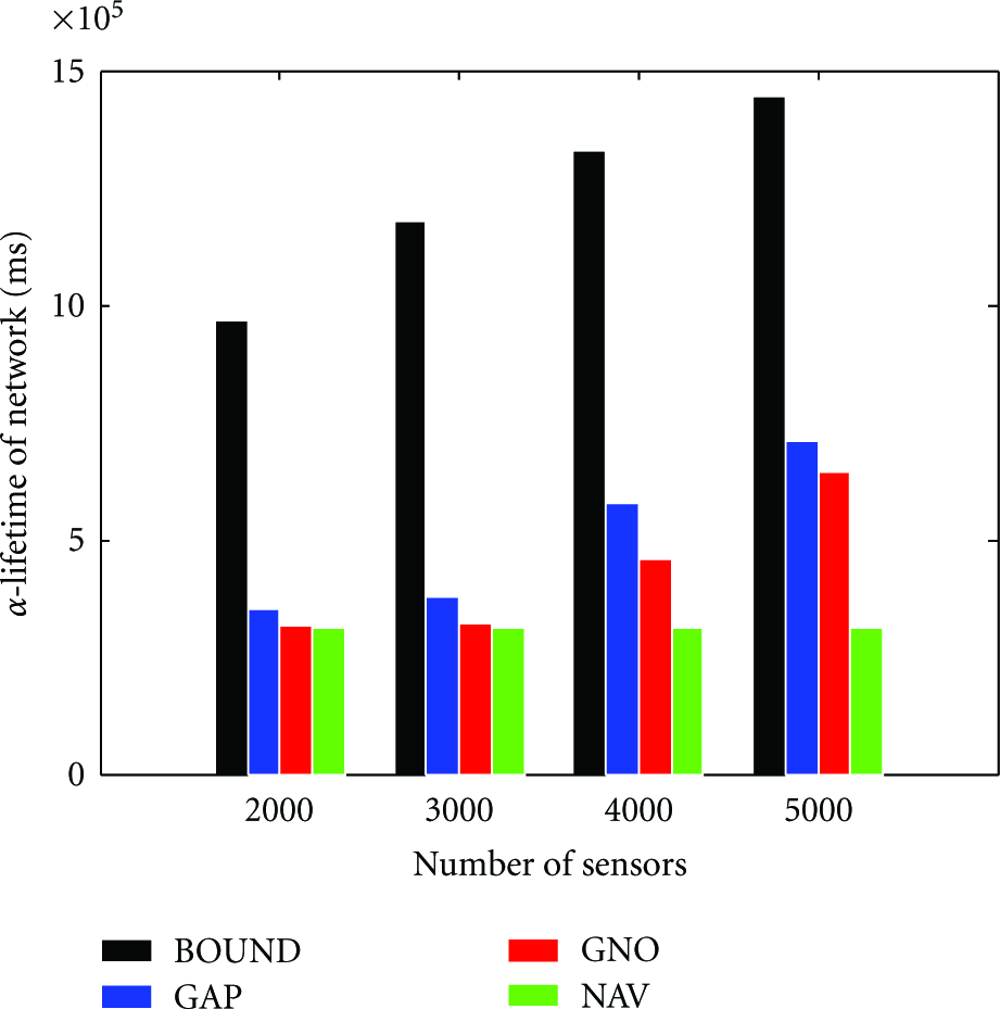
Comparison of 90-lifetime of network.

Figure 13

Comparison of 70-lifetime of network.

Figure 14

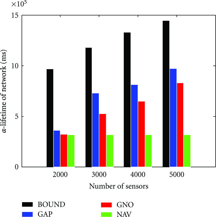
Comparison of 50-lifetime of network.

6. Discussions

Unreliable Links

It has been well known that wireless transmissions are unreliable. In GAP, the broadcasting of an UPDATE is important. Suppose that sensor Q broadcasts its new probability and reduces its active probability accordingly. Sensor B, a detection neighbor of Q, fails to receive the packet from Q. In this case, there may occur a violation since B still keeps the previous probability of Q that is larger than the current real active probability of Q. Based on this out-of-date information, B may calculate a new probability that fails to ensure that the detectability of some point within its detection range.

However, we should point out that the detection range is usually much shorter than the communication range. According to the data measured on eXtreme Scale Mote, the detection range of magnetic sensor detecting vehicles are 8 m. The communication range of a Mica2 Mote [23] is about 150 m in the outer door environment. It has been revealed that two sensor nodes that close to each other have much more reliable packet transmission. On the other hand, we can introduce an additional duplicate packet immediately following the previous one to confirm the update packet. This can further mitigate the problem that can be introduced by occasional failures of UPDATE reception, if the environment is harsh for wireless communication.

Inaccurate Locations

In the design of GAP, location information has been crucial. The accuracy of location information of sensor nodes certainly impacts the performance of the algorithm. If the estimated location is inaccurate, a sensor fails to precisely identify the set of grid points that are really within its detection range and the set of detection neighbors. The consequence is that the system may fail to provide guaranteed detectability.

Fortunately, we are able to address the problem introduced by inaccurate location if location errors are insignificant. On one hand, we have witnessed rapid advances in technologies for positioning sensor nodes accurately. Recently, study has reported that localization with accuracy of several centimeters has been possible [25]. On the other hand, we can use a more conservative nominal detection range to compensate the inaccuracy introduced by location errors.

7. Conclusion and Future Work

In this paper, we have presented the GAP algorithm that provides guaranteed detectability for any event occurring in the sensing field. GAP exposes a convenient interface for the user to specify the desired detectability. Employing the probabilistic approach, GAP is able to finely tune the active probability of each sensor so as to minimize the power consumption of the sensors. The algorithm does not rely on costly time synchronization and is fully distributed, therefore truly scalable to network scale and sensor density. It has demonstrated through simulation experiments that GAP significantly prolongs system lifetime while satisfying the specified detectability for any event.

The future work will proceed in several important directions. First, we plan to further study the impact of inaccurate location and unreliable wireless communications on detection performance and the necessary design that should be enhanced. Second, we will implement the algorithm in a testbed to validate the design and to study its performance under realistic complex environments.