
Abstract
MHD free convection and mass transfer flow over a continuously moving vertical porous plate under the action of strong magnetic field is investigated. In this analysis the hall and ion-slip current in the momentum equation are considered for high speed fluid flows and the level of concentration of foreign mass have been taken very high. The governing equations of the problem contain a system of partial differential equations. The coupled partial differential equations are solved numerically by explicit finite difference method. The results of this investigation are discussed for the different values of the well-known parameters with different time steps. Finally, the obtained finite difference solutions are compared with analytical solution by the graphical representation.
1. Introduction
The use of magnetic field that influences mass generation process in electrically conducting fluid flows has important engineering applications. Hall currents effects are likely to be important in many astrophysical and geophysical situations as well as in engineering problems such as Hall accelerators, constructions of turbines, and centrifugal machines. The effects of Hall and ion-slip currents in steady MHD free convective flow past a semi-infinite vertical porous plate in a rotating frame of reference when the heat flux maintained as constant at the plate was studied by Ram. Takhar and Ram [1] investigated the effects of hall current on hydromagnetic free convective flow through a porous medium. Later, they dealt with MHD free convection from an impulsively moving infinite vertical plate in a rotating fluid with Hall and ion-slip currents. Pop and Watanable studied the effects of Hall current on MHD free convection flow past a semi-infinite vertical flat plate. The effects of Hall and ion-slip currents on free convective heat generating flow in a rotating fluid were analysed by Ram. Abo-Eldahab and El Aziz [2] studied the hall and ion-slip effects on MHD free convective heat generating flow past a semi-infinite vertical flat plate. Seddeek and Abdelmeguid [3] studied hall and ion-slip effects on magnetomicropolar fluid with combined forced and free convection in boundary layer flow over a horizontal plate. Abo-Eldahab and El Aziz [4] investigated viscous dissipation and Joule heating effect on MHD free convection from a vertical plate with power law variation in surface temperature in the presence of Hall and ion slip currents. In the present study, the transient flow and mass transfer of a viscous incompressible electrically conducting fluid within a vertical semi-infinite porous plate is studied with the consideration of both the Hall current and ion slip currents. Finally, nondimensional coupled similar and nonsimilar equations are solved by explicit finite difference method. Numerical results have presented for the range of Prandtl number, Schmidt Number, and other well-known parameters which are taken arbitrarily for the fluid.
2. Mathematical Formulation
The plate as well as the fluid is considered at the same temperature and the concentration level everywhere in the fluid is the same.
Also it is assumed that the fluid and the plate are at rest; after that the plate is moving with a constant velocity U in its own plane and instantaneously at time

Geometrical configuration of thermal boundary layer.
(I) All the physical properties of the fluid are considered to be constant excepttheinfluenceofvariationsof density with temperature which considered only on the body force term, in accordance with the Boussinesq's approximation.
(II) Since the plate is of semi infinite extent and the fluid motion is unsteady so all the flow variables will depend only upon y and time
(III) The hall and ion slip terms in the momentum equation are considered for observing the pattern of velocity variation.
(IV) The equation of conservation of electric charge,

where

For the strong magnetic field Lorentz force becomes
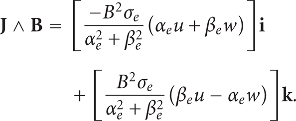
Within the framework of the above-stated assumptions the generalized equations relevant to the one-dimensional unsteady free convective mass transfer problem are governed by the following system of coupled partial differential equations.
Momentum Equation in x-Direction
Consider that

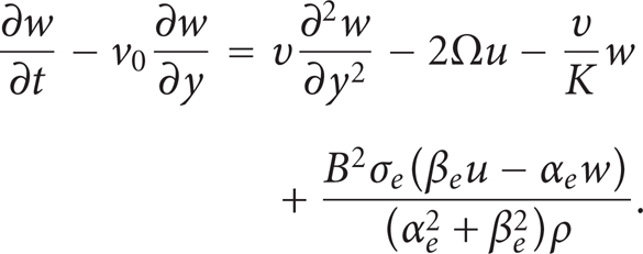
Momentum Equation in z-Direction
Consider that
Energy Equation
Consider that

Concentration Equation
Consider that

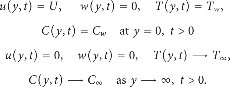
with the corresponding initial and boundary conditions are

Since the solutions of the governing (4) to (7) under the initial conditions (8) and boundary conditions (9) will be based on the finite difference method it is required to make the equations dimensionless. For this purpose we now introduce the following dimensionless quantities:

Applying all those nondimensional variables into the equations (4) to (7), the basic equations relevant to the problem are in dimensionless form

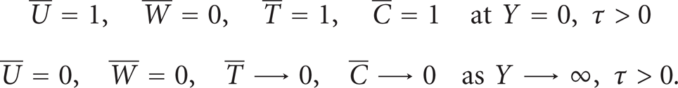
with the corresponding initial and boundary conditions are

The nondimensional quantities introduced in (11) are defined as

3. Shear Stress, Nusselt Number, and Sherwood Number
From the velocity field, the effects of various parameters on the plate shear stress have been calculated. The following equations represent the shear stress at the plate.
Shear stress
From the temperature field, the effects of various parameters on the heat transfer coefficients have been analysed. The following equations represent the heat transfer rate that is well-known Nusselt number.
Nusselt number
And from the concentration field, we analyze the effects of various parameters on the mass transfer coefficients. The following equation represents the mass transfer rate that is well-known Sherwood number.
Sherwood number
4. Numerical Solutions
In this section, we attempt to solve the governing second-order coupled dimensionless partial differential equations with the associated initial and boundary conditions. For simplicity the explicit finite difference method has been used to solve (11) subject to the initial and boundary conditions (12) and (13). The present problem requires a set of finite difference equation. In this case the region within the boundary layer is divided by some perpendicular lines of
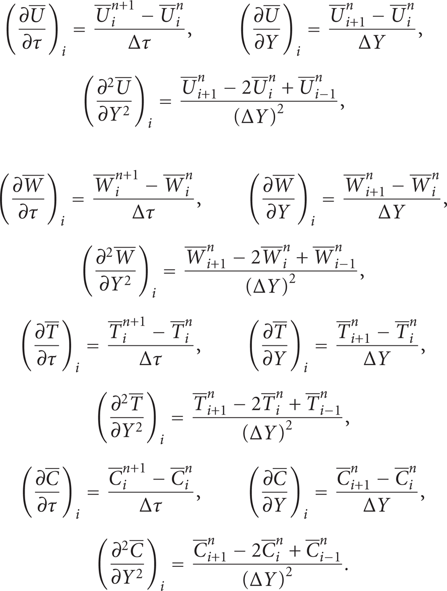
From the system of partial differential equation (11) with substituting the above relations into the corresponding differential equation we obtain an appropriate set of finite difference equations,


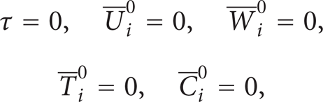
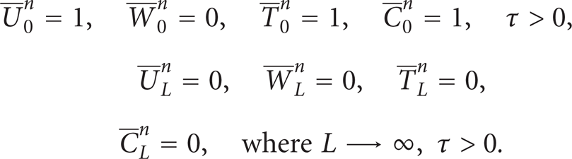
and the initial and boundary conditions with the finite difference scheme are
Here the subscripts i designate the grid points with Y coordinates and the superscript n represents a value of time,
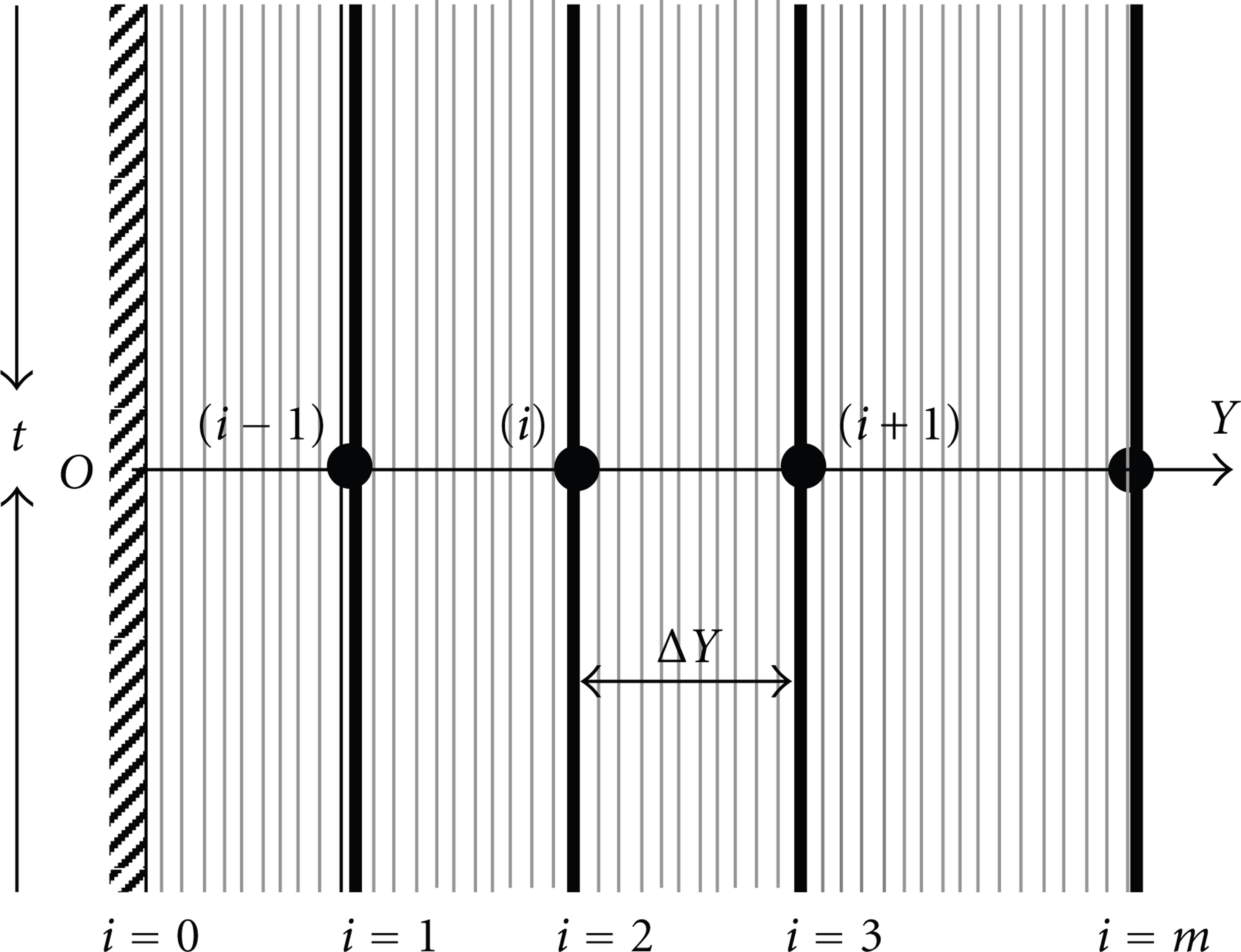
Finite difference space grid.
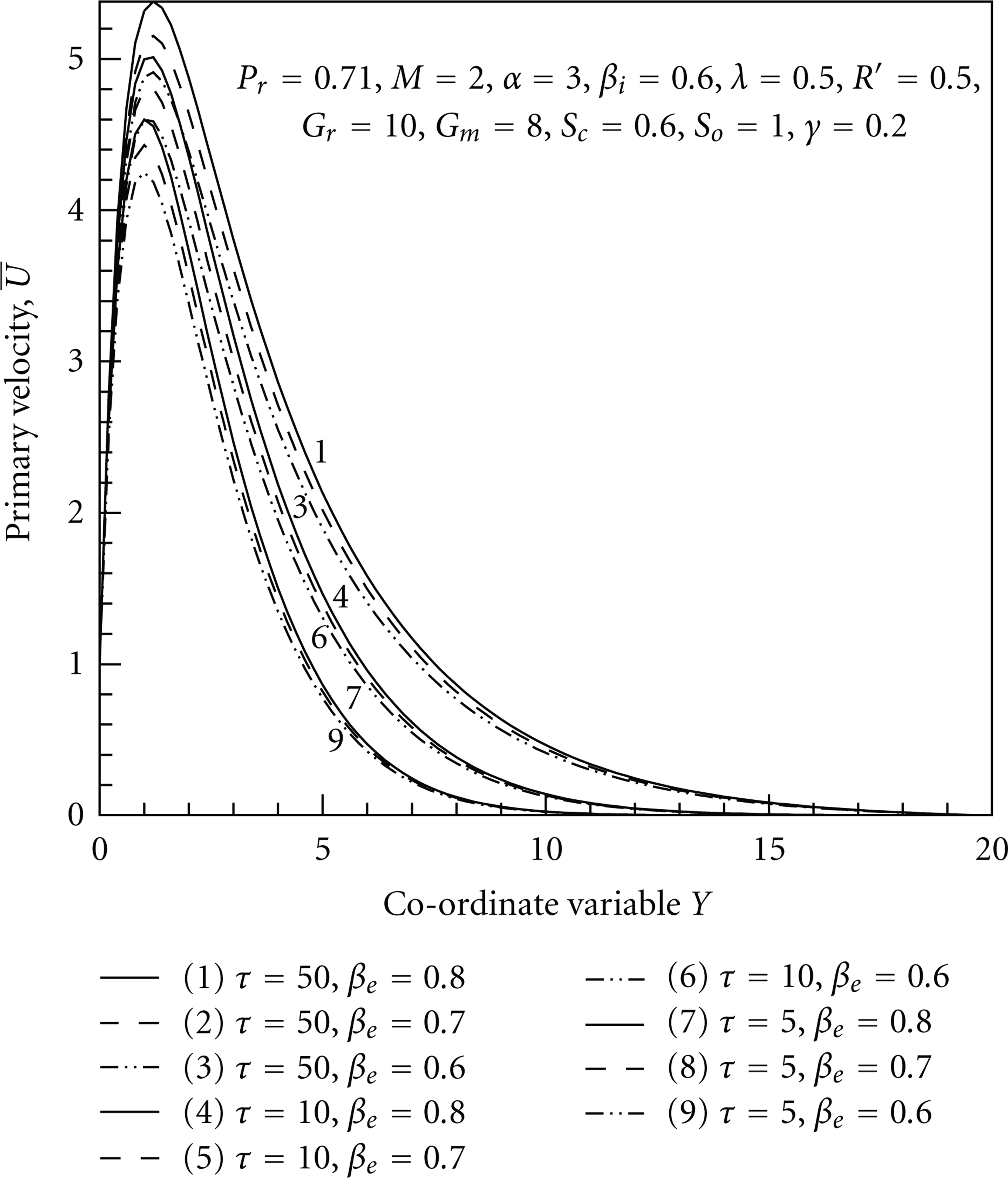
Primary velocity profile for different value of hall parameterβ e with τ = 5, τ = 10, andτ = 50.
5. Stability and Convergence Analysis
Since an explicit procedure is being used, the analysis will remain incomplete unless we discuss the stability and convergence of the finite difference scheme. For the constant mesh sizes the stability criteria of the scheme may be established as follows.
The general terms of the Fourier expansion for
and after the time step these terms will become

Substituting (22) and (23) into (22) to (25), we obtain the following equations upon simplification:


Equations (24), (25), (26), and (27) can be written in the following form:

where

Equations (28) may be expressed in matrix form as follows:
that is,

From the above matrix T we obtain the following eigenvalues:

For stability, each eigenvalue

We have

or,

where
The coefficients a, b, and c are all real and nonnegative. We can demonstrate that the maximum modulus of Joccurs when

or

To satisfy the first condition

or,
Same calculation applied for the second condition

as well as

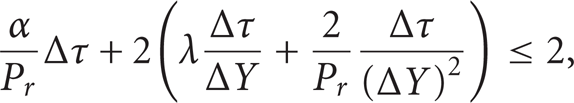
Hence, the stability conditions of the problem are as furnished below

Form the above equations (42) the convergence limit for the model of flow are
6. Results and Discussion
In case of observing the physical significance of the model, the numerical values of primary velocity
The transient primary and secondary velocity profiles have been shown in Figure 3 to Figure 18 for different values of β
e
, β
i
, M, S
o
, R′,P
r
, λ, S
c
in case of cooling plate. The effect of hall parameter β
e
as well as for the different values of τ is represented for the primary velocity distribution in Figure 3. In this figure we observe that the primary velocity decreases with the decrease of hall parameter β
e
but as compare to τ the primary velocity increases with the increase of τ. In Figure 4, for τ = 5, τ = 10, and τ = 50, the secondary velocity increases for the decrease of hall parameter β
e
. From Figure 5, we analyze that the primary velocity has a minor effect with the decrease of ion-slip parameter β
i
. But the secondary velocity increases gradually with the decrease of ion-slip parameter β
i
in Figure 6. The effect of the magnetic parameter on the velocity profile is represented in Figure 7. It is observed that

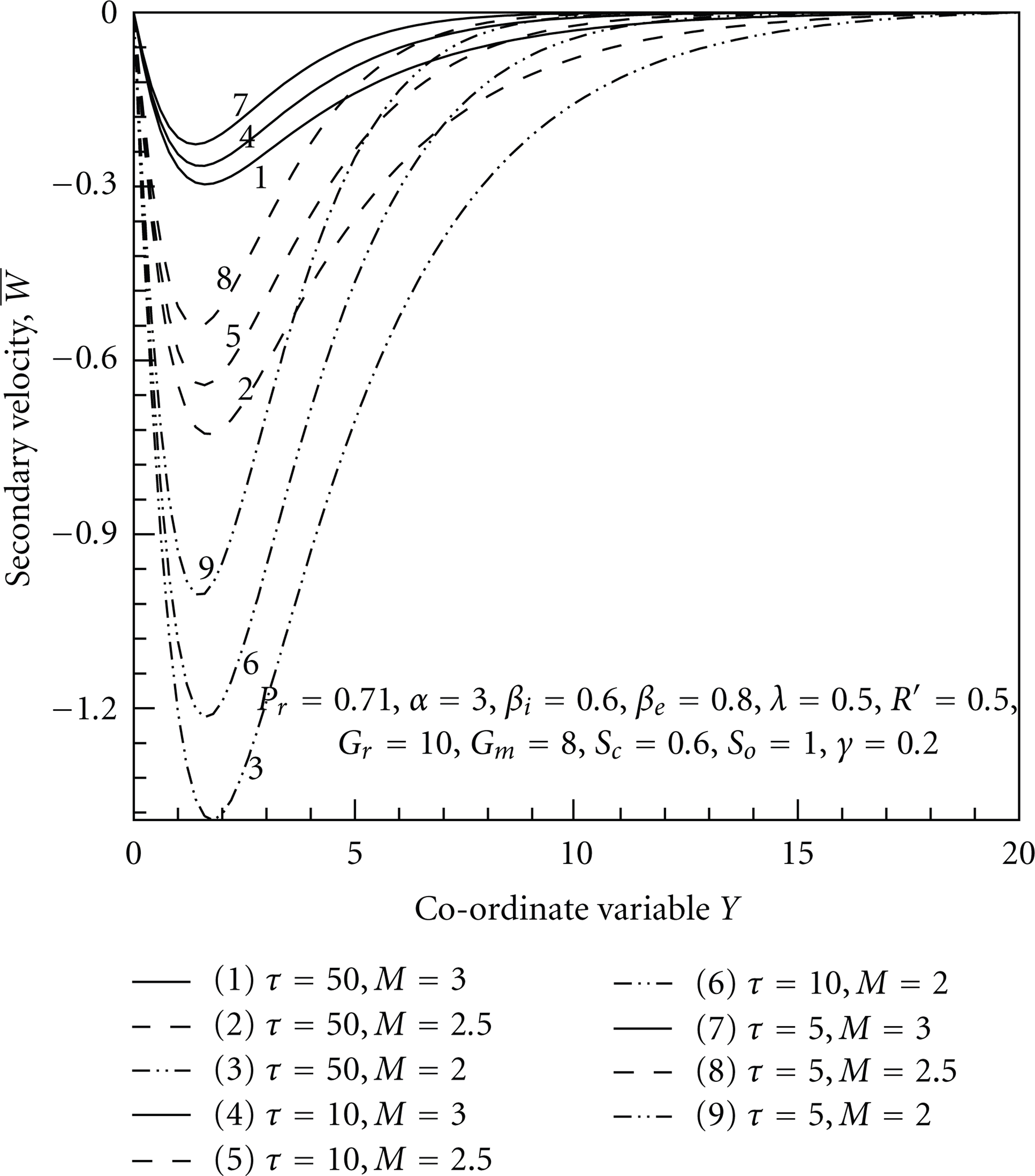
Secondary velocity profile for different value of hall parameter β e with τ = 5, τ = 10, and τ = 50.
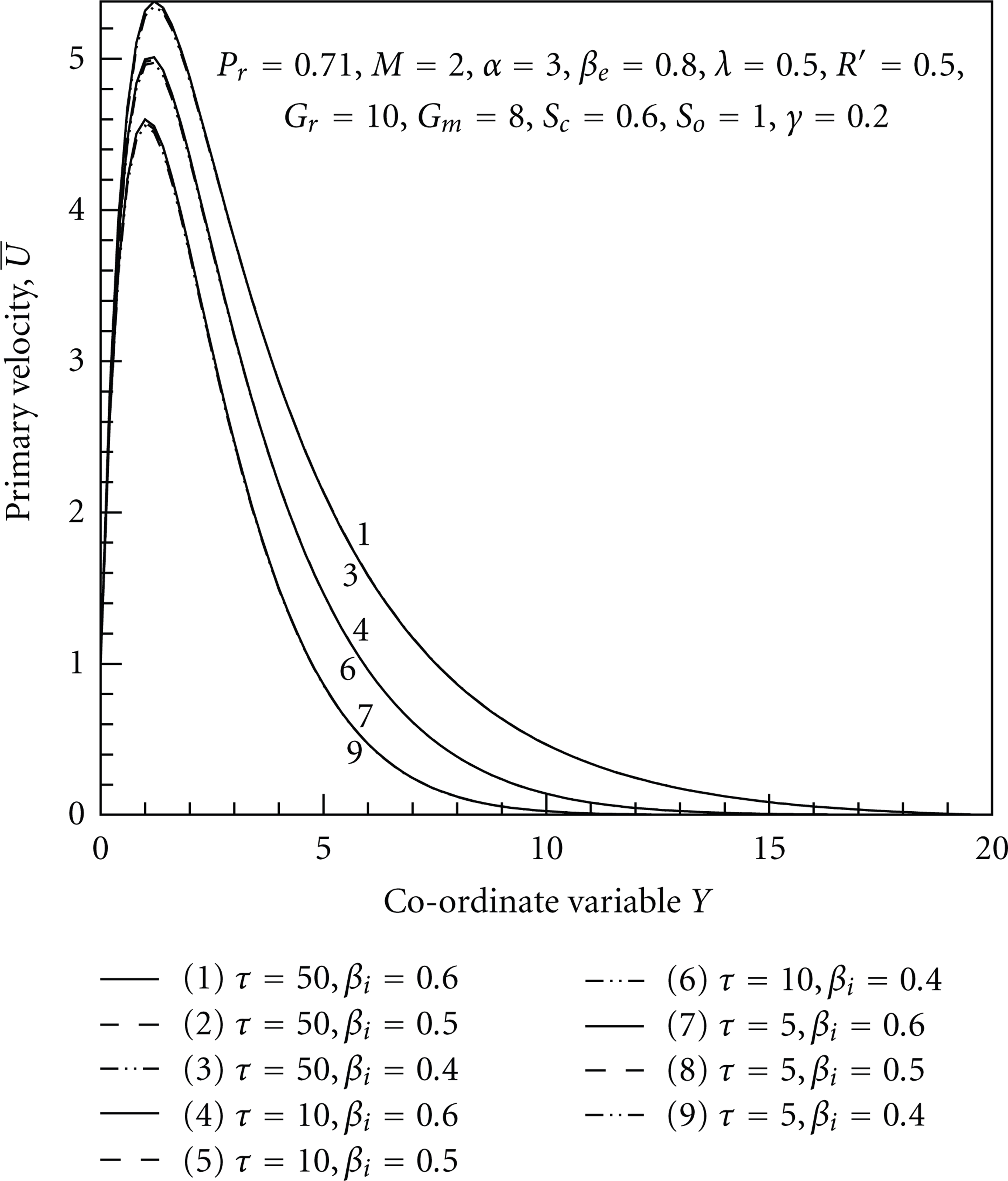
Primary velocity profile for different value of ion-slip parameter β i with τ = 5, τ = 10, and τ = 50.
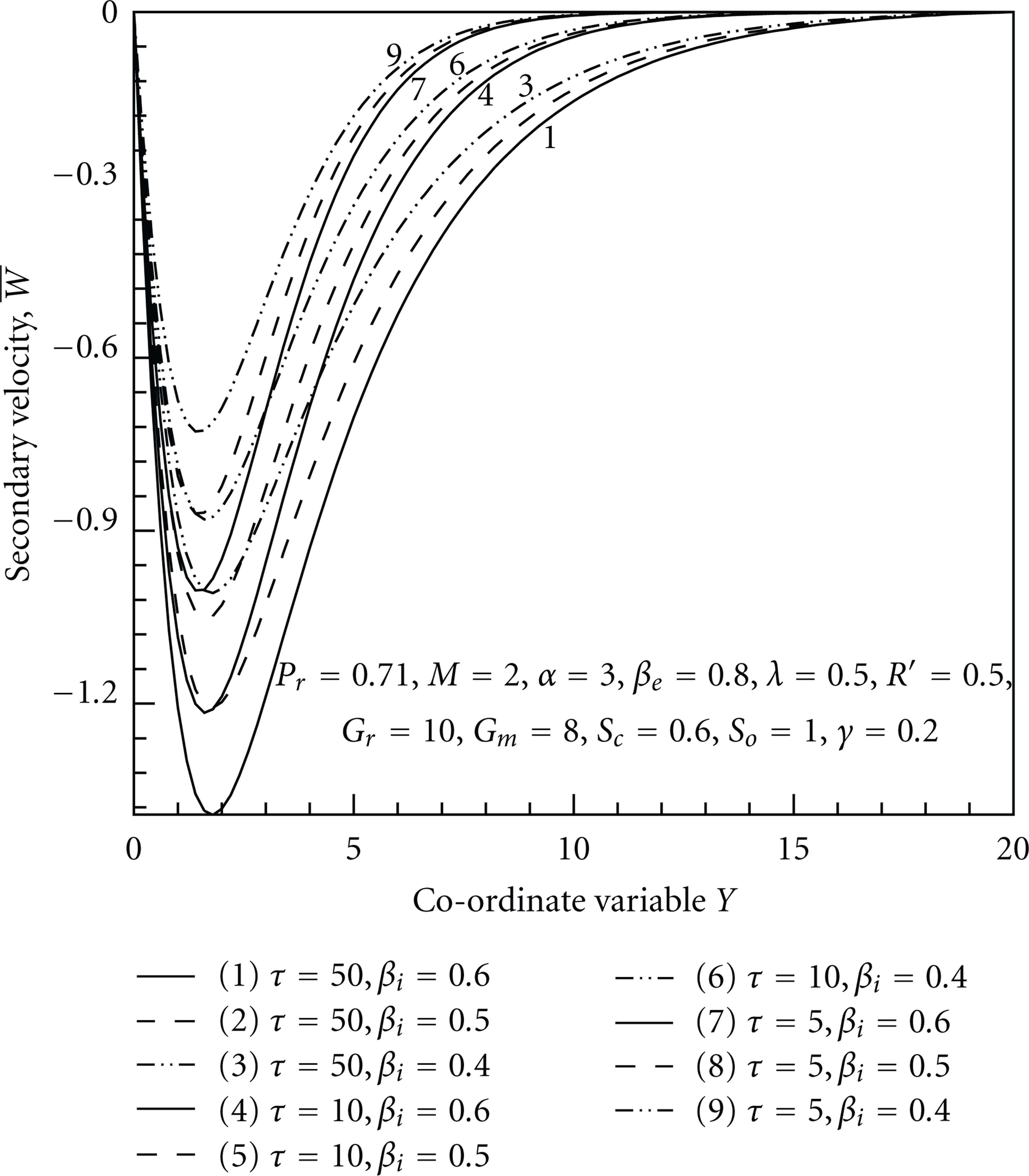
Secondary velocity profile for different value of ion-slip parameterβ i withτ = 5, τ = 10, and τ = 50.
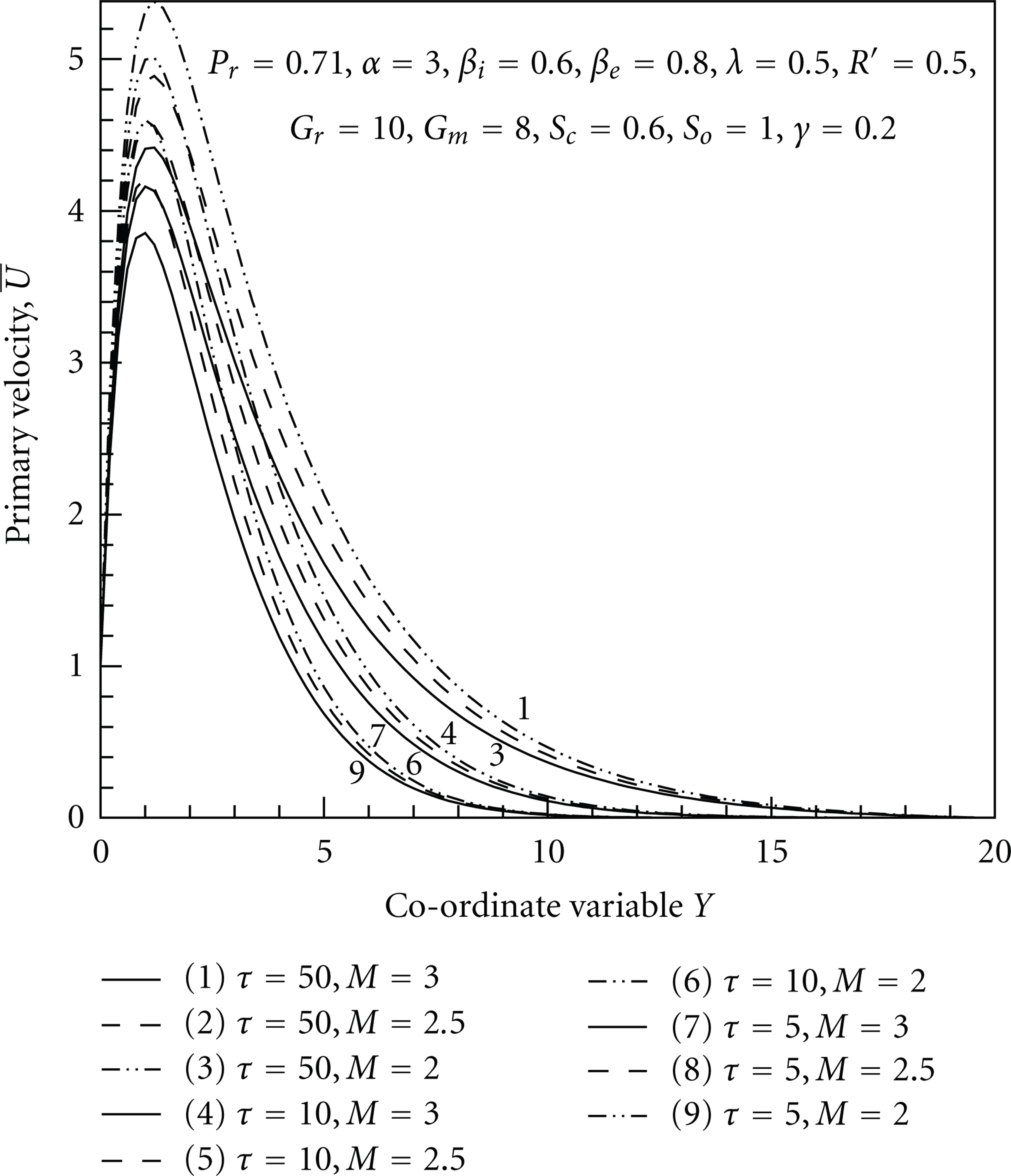
Primary velocity profile for different value of magnetic parameterMwithτ = 5, τ = 10, and τ = 50.
Secondary velocity profile for different value of magnetic parameterMwithτ = 5, τ = 10, and τ = 50.

Primary velocity profile for different value of rotational parameterR′with τ = 5, τ = 10, and τ = 50.
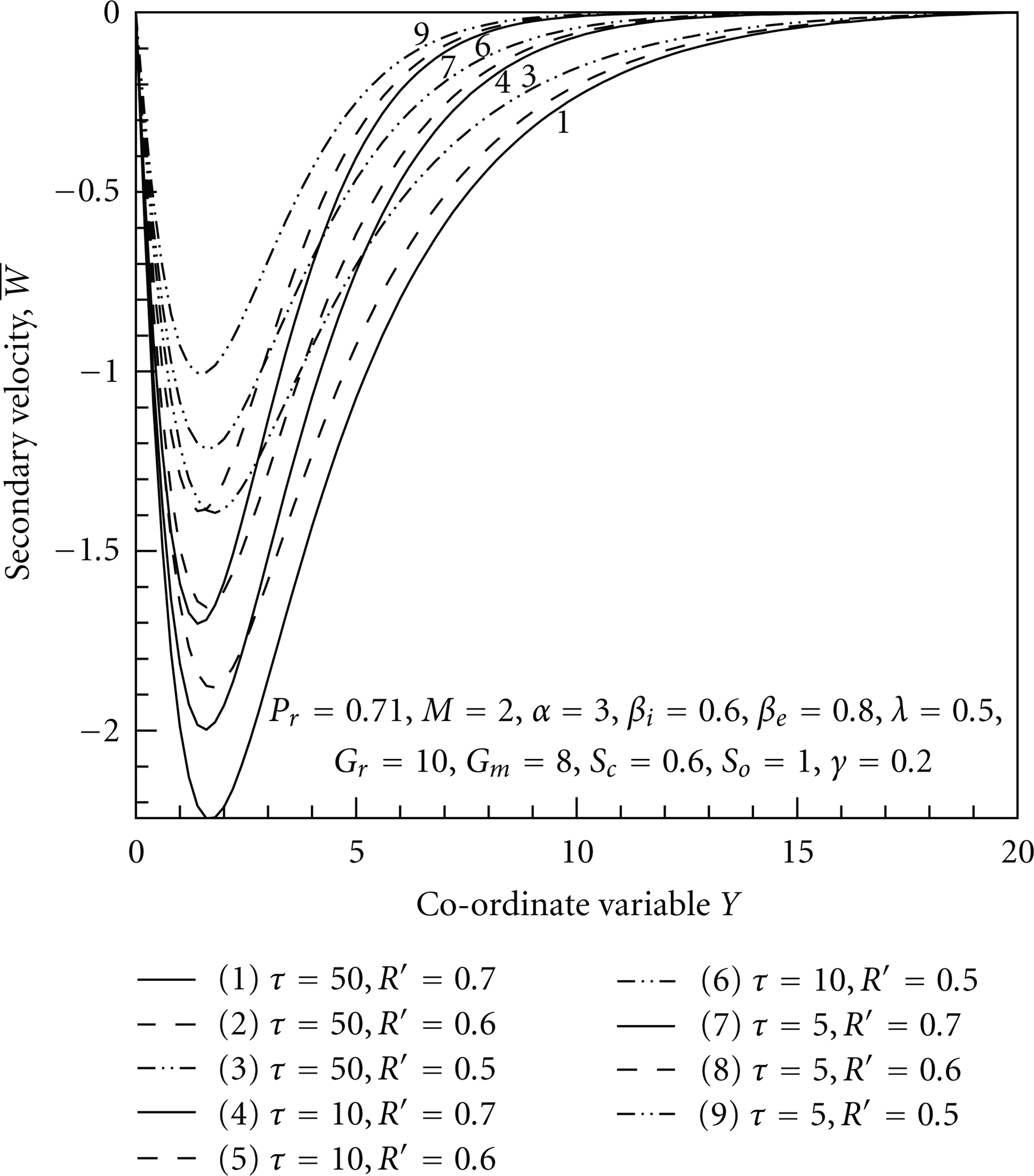
Secondary velocity profile for different value of rotational parameterR′ with τ = 5, τ = 10, and τ = 50.

Primary velocity profile for different value of Prandtl parameter P r with τ = 5, τ = 10, and τ = 50.
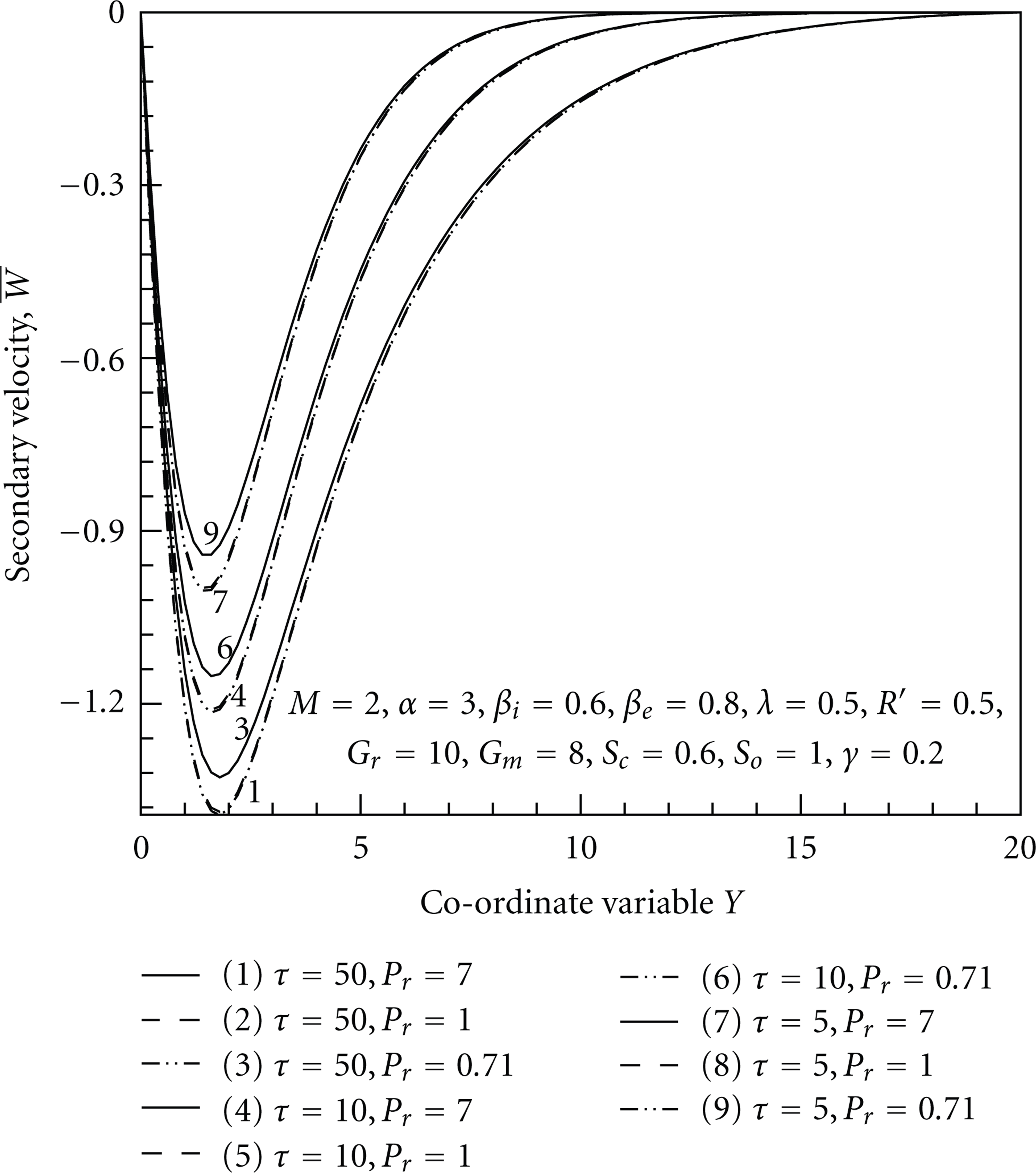
Secondary velocity profile for different value of Prandtl parameter P r with τ = 5, τ = 10, and τ = 50.

Primary velocity profile for different value of suction parameter λwith τ = 5, τ = 10, and τ = 50.

Secondary velocity profile for different value of suction parameter λ with τ = 5, τ = 10, and τ = 50.

Primary velocity profile for different value of Schmidt number S c with τ = 5, τ = 10, and τ = 50.

Secondary velocity profile for different value of Schmidt number S c with τ = 5, τ = 10, and τ = 50.

Primary velocity profile for different value of Soret number S o with τ = 5, τ = 10, and τ = 50.

Secondary velocity profile for different value of Soret number S o with τ = 5, τ = 10, and τ = 50.
Now we analyze shear stress

Shear stress τ x for different values of hall parameter β e .

Shear stress τ z for different values of hall parameter β e .

Shears tress τ x for different values of ion-slip parameterβ i .

Shear stress τ z for different values of ion-slip parameterβ i .

Shear stress τ x for different values of magnetic parameter M.

Shear stress τ z for different values of magnetic parameterM.

Shear stress τ x for different values of Soret numberS o .

Shear stress τ z for different values of Soret numberS o .

Shear stress τ x for different values of heat source parameterα.

Shear stress τ z for different values of heat source parameterα.
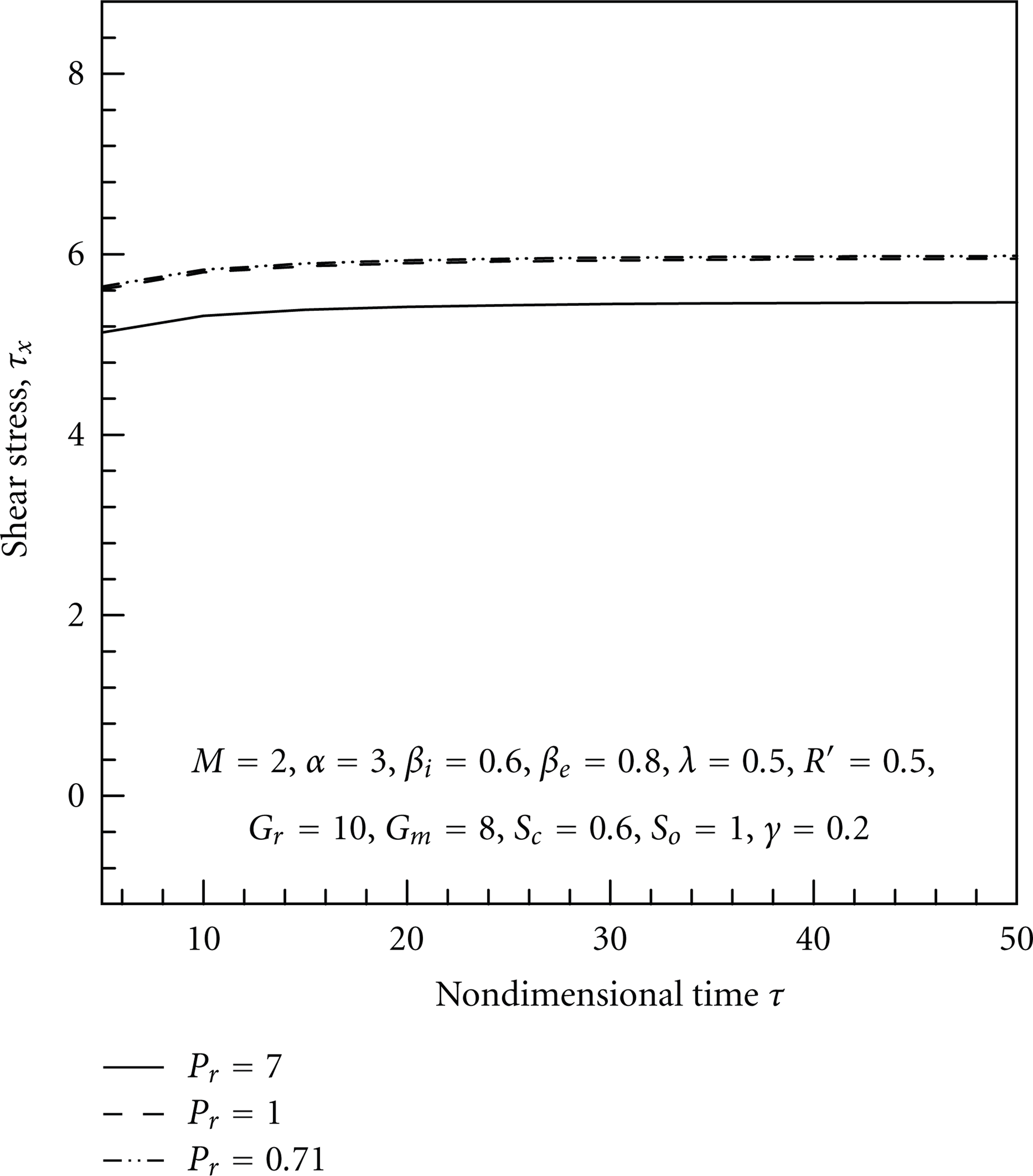
Shear stress τ x for different values of Prandtl numberP r .

Shear stress τ z for different values of Prandtl numberP r .

Shear stressτ x for different values of suction parameter λ.

Shear stress

Shear stressτ x for different values of Schmidt numberS c .
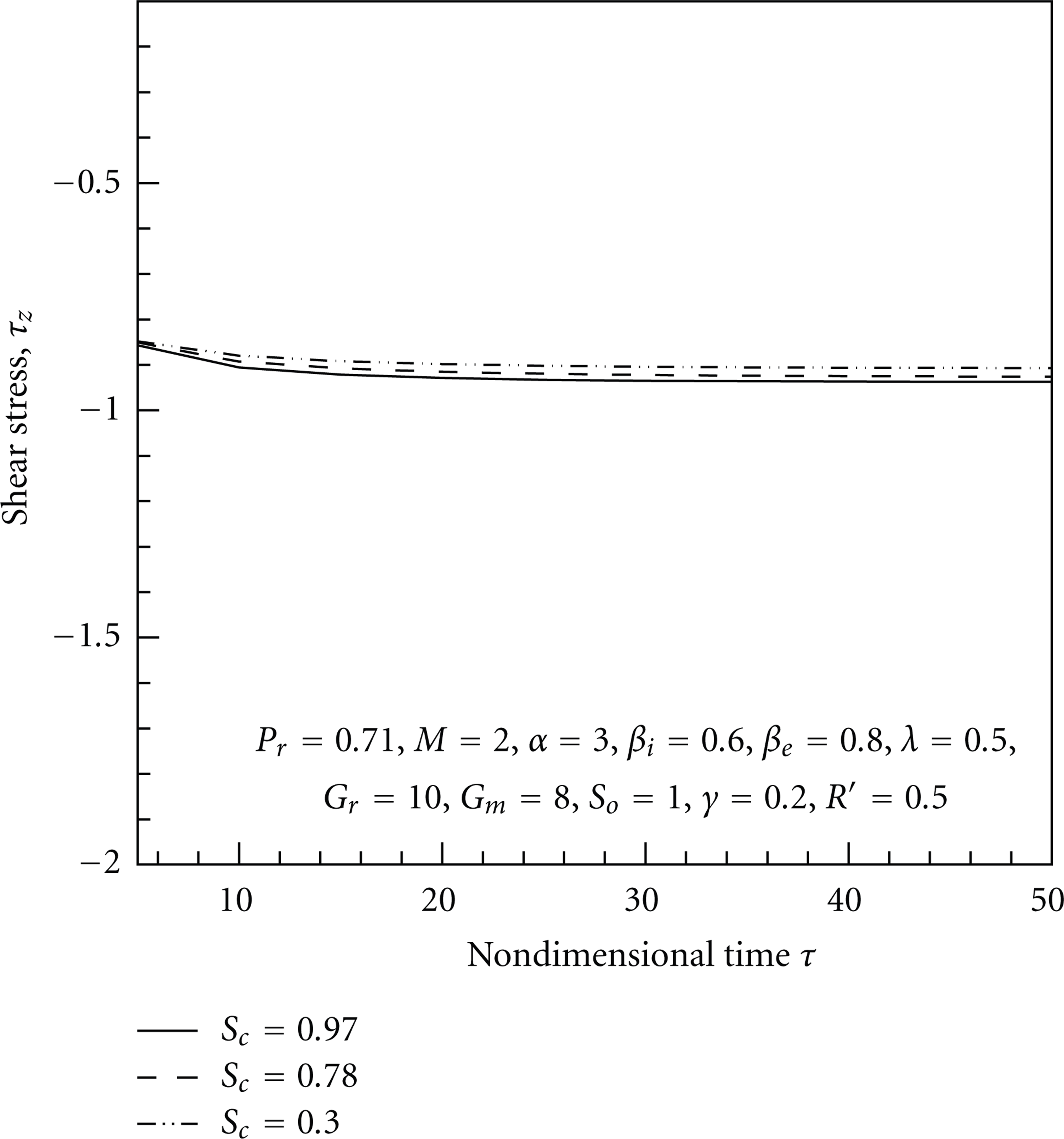
Shear stressτ z for different values of Schmidt numberS c .
In Figures 35 and 36, Nusselt number N u has shown for the effect of suction parameter λ and Prandtl number P r respectively. For both the case Nusselt number N u decreases with the decrease of suction parameter λ and prandtl number P r . The profiles for Sherwood number S h for the different values of prandtl number P r and Schmidt number S c are represented in Figures 37 and 38, where Sherwood number S h has increasing effect on decrease of prandtl number P r and Schmidt number S c .

Nusselt number N u for different values ofsuction parameterλ.

Nusselt number N u for different values of Prandtl number P r .
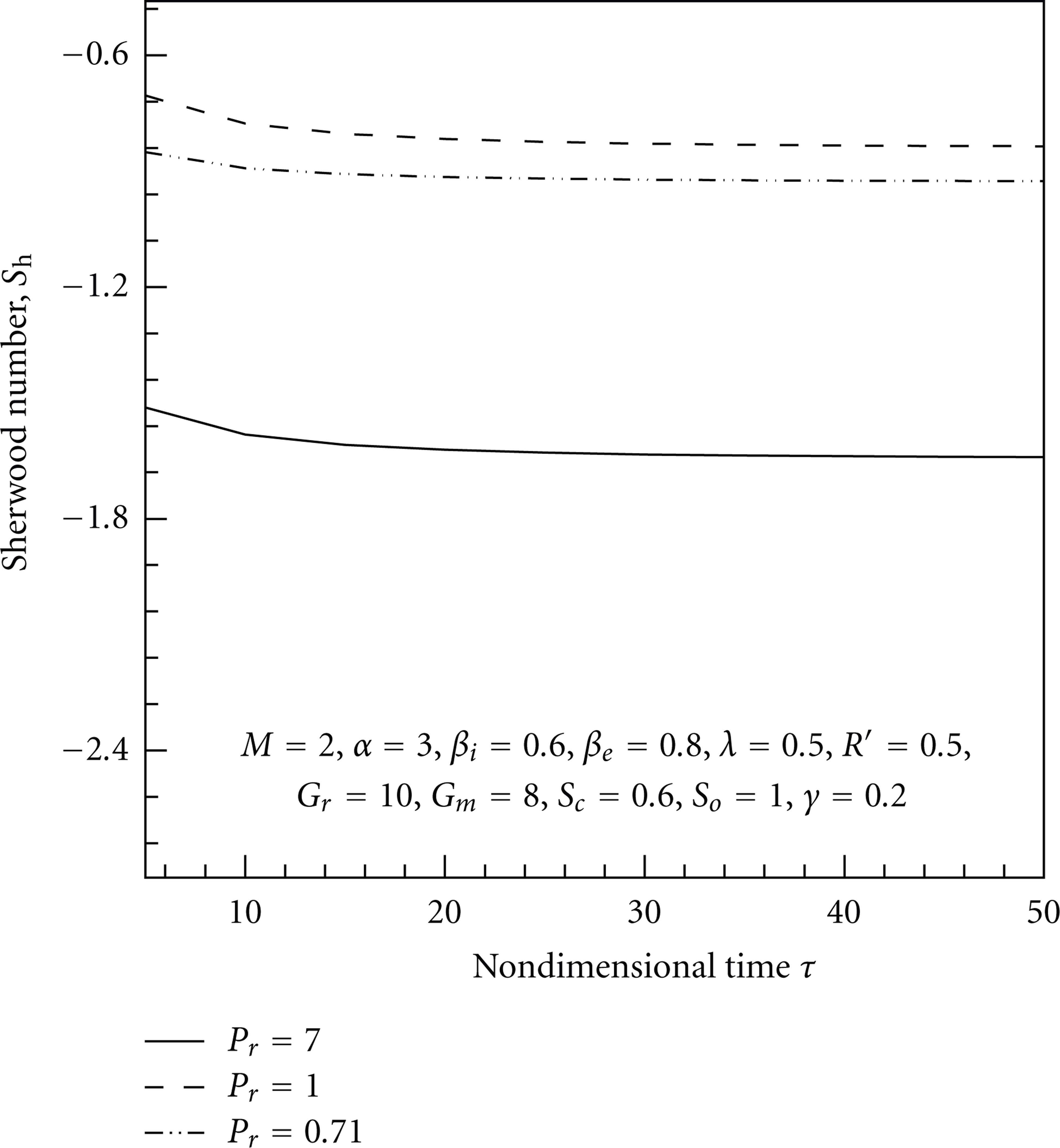
Sherwood number S h for different values of Prandtl numberP r .
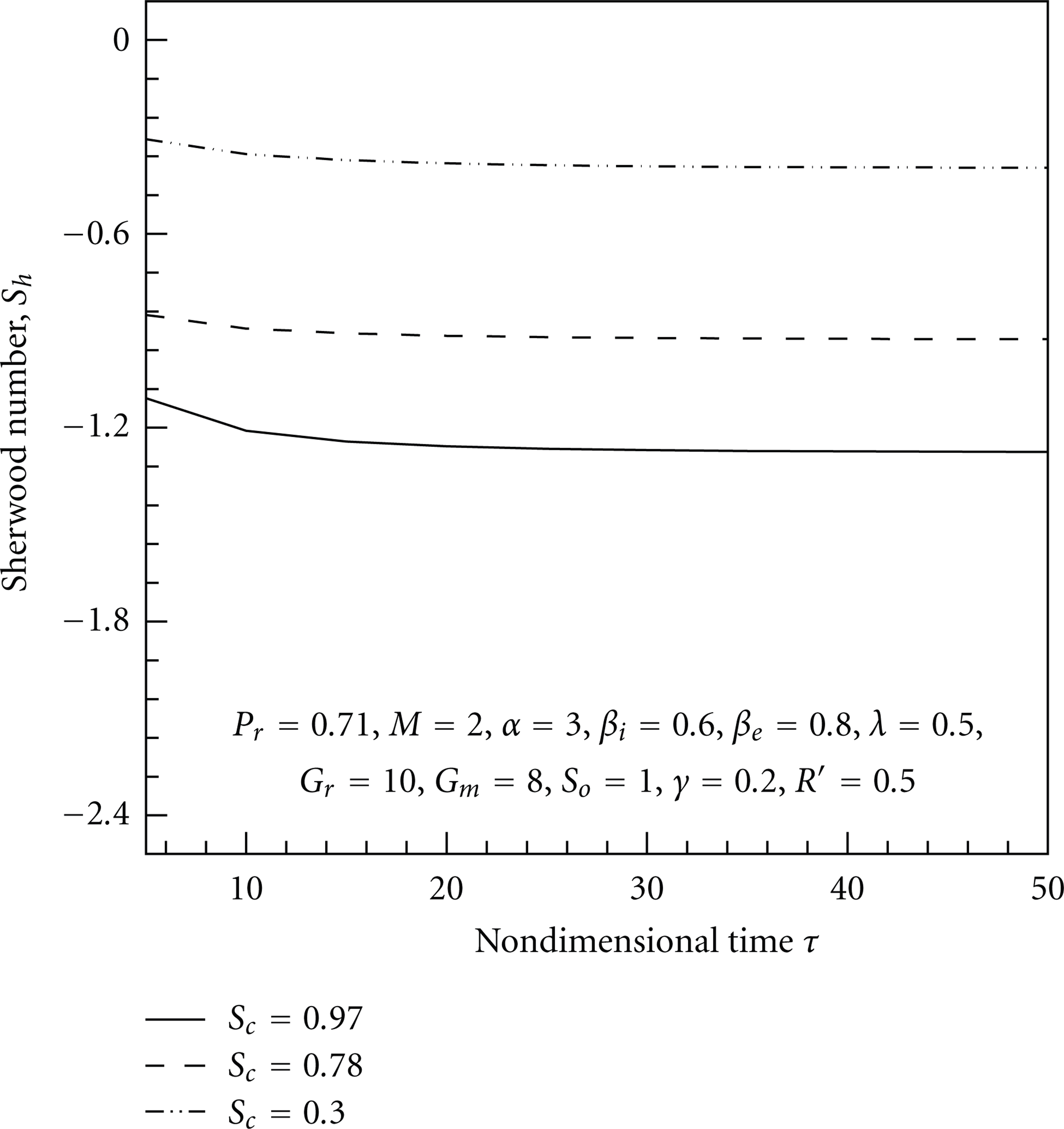
Sherwood number S h for different values of Schmidt number S c .
7. General Discussions
A differential equation is a mathematical equation for an unknown function of one or several variables that relates the values of the function itself and its derivatives of various orders. Differential equations are mathematically studied from several different perspectives, mostly concerned with their solutions. We can solve differential equations on both analytical and numerical way (Figures 39, 40, 41, 42, 43, and 44). In some of the cases all the problems are impossible to solve in analytical way. But numerical process is more acceptable in that case. In this chapter we discussed about the comparison between analytical and finite difference solution with graphical representation within the perspective of our problem.

(a) Analytical solution of primary velocity profile for different value of hall parameter β e . (b) Numerical solution of primary velocity profile for different value of hall parameter β e .

(a) Analytical solution of secondary velocity profile for different value of hall parameter β e . (b) Numerical solution of secondary velocity profile for different value of hall parameter β e .

(a) Analytical solution of primary velocity profile for different value of magnetic parameter M. (b) Numerical solution of primary velocity profile for different value of magnetic parameter M.

(a) Analytical solution of secondary velocity profile for different value of magnetic parameter M. (b) Numerical solution of secondary velocity profile for different value of magnetic parameter M.

(a) Analytical solution of temperature profile for different value of heat source parameter α. (b) Numerical solution of temperature profile for different value of heat source parameter α.

(a) Analytical solution of concentration profilefor different value of Schmidt number S c . (b) Numerical solution of concentration profile for different value of Schmidt number S c .
8. Comparison
To obtain a considerable comparison the same parametric values with the steady-state condition for both analytical and numerical solution are taken. In Comparison Figure 29(a) and Comparison Figure 29(b) primary velocity profile for different values of hall parameter β e shown by applying analytic and finite difference method, respectively, for both cooling and heating of the porous plate, where we observe that the primary velocity is decreased with the decrease of hall parameter β e for cooling of the plate in both of the two Comparison Figures 29(a) and 29(b); for heating of the plate the primary velocity is increased with the decrease of hall parameter β e . Comparison Figures 30(a) and 30(b) represents the secondary velocity profile for analytic and finite difference method, respectively, within both the case of cooling and heating plate, where secondary velocity profile shows the same characteristics for the solution of analytic and finite difference method. Comparison Figures 31(a) and 31(b) represent the primary velocity profile and Comparison Figures 32(a) and 32(b) represent the secondary velocity profile respectively for different values of magnetic parameter M, where for the analytic and numerical solution both the primary and secondary velocity acted towards the same flow pattern. Comparison Figures 33(a) and 33(b) represent that temperature profile is increases with the decrease of heat source parameter α for both the case of analytic and numerical solutions. Comparison Figures 34(a) and 34(b) illustrate that for the decreases of Schmidt number S c concentration profile reacts exactly the same for analytic and finite difference solution.
From the above discussion, the analytical and the numerical solutions of primary velocity profile, secondary velocity profile, transiesnt temperature profile, and transient concentration profile have comparatively similar flow pattern for different parameters.
9. Conclusions
MHD mass transfer problem by free convection flow of an electrically conducting incompressible viscous fluid past an electrically conducting continuously moving semi-infinite vertical porous plate under the action of strong magnetic field is taken into account. The resulting governing system of dimensionless coupled nonlinear partial differential equations are numerically solved by an explicit finite difference method. The results are discussed for different values of important parameters as hall parameter, ion slip parameter, magnetic parameter, rotational parameter, heat source parameter, Soret number, Grashof number, modified Grashof number, Prandtl number, and Schmidt number. The important findings of this investigation with graphical representation are listed below.
The primary velocity increases with the decrease of M, R′, P r , λwhile the transient primary velocity decreases with the decrease of β e , β i , G r , G m .
The secondary velocity increases with the decrease of β e , β i , G r , G m while the transient secondary velocity decreases with the decrease of M, P r , λ.
The transient temperature increases with the decrease of α and λ. Particularly, the fluid temperature is more for air than water and it is less for lighter than heavier particles.
The transient concentration profiles are increasingly affected by P r , λ and decreasingly affected by S o , also α has a minor effect for concentration profile. Particularly, the species concentration is higher for water than air as well as it is more for lighter than heavier particles.
The shear stress τ x increases with the decrease of M, α, P r , λ while it decreases with the decrease of β e , β i , G r , S o , S c , G m .
The shear stress τ z decrease with the decrease of M, α, P r , λ, while it increases with the decrease of β e , β i , G r , S o , S c , G m . The shear stress is greater for air than water.
The rate of heat transfer increase with the increases of Prandtl number P r and suction parameter λ. The rate of heat transfer is higher for water than air.
The rate of mass transfer increases with the decrease of P r , S o and S c . The coefficient of mass transfer is greater for heavier than lighter particles. On the opposite case mass transfer has a decreasing effect with the decrease of λ.
In this analysis the effect of different parameters on the velocity, temperature, and concentration flow pattern is discussed. In all those parameters hall and ion slip terms are the main objective for our work, which has attracted the interest of any investigators in view of its important applications in many engineering problems such as power generators, MHD accelerators, refrigeration coils, transmission lines, electric transformers, and heating elements. Also the comparison between analytical and numerical solution gives clear information about the work.