Secrecy Transfer

Abstract

Suppose that n nodes with $n_0$ acquaintances per node are randomly deployed in a two-dimensional Euclidean space with the geographic restriction that each pair of nodes can exchange information between them directly only if the distance between them is at most r, the acquaintanceship between nodes forms a random graph, while the physical communication links constitute a random geometric graph. To get a fully connected and secure network, we introduce secrecy transfer which combines random graph and random geometric graph via the propagation of acquaintanceship to produce an acquaintanceship graph $G_{n,n_0}$ , a kind of random geometric graph with each edge representing an acquaintanceship between two nodes. We find that components of graph $G_{n,n_0}$ that undergoes a phase transition from small components to a giant component when $n_0$ is larger than a threshold, the threshold for $G_{n,n_0}$ to be a connected graph is derived. In addition, we present its implementation method and applications in wireless sensor networks.

1. Introduction

Suppose at a classroom with n students, each of whom initially has $n_{\mathrm{0}}$ acquaintances who are randomly chosen among them. Students can only communicate with its direct neighbors. At first, students are isolated. If two adjacent students are acquainted with each other, a link forms between them. As time goes on, some small acquaintance groups emerge. Two stranger students, say Alice and Bob, belonging to different groups may be adjacent, but if there are students in the two groups, respectively, familiar with each other, Alice and Bob may use them as introducers to establish a link between them. By repeating this process, students will be increasingly interwoven by such links, creating a web of acquaintances. We denote this construction as secrecy transfer and the resulting network as the acquaintanceship graph $G_{n,n_{\mathrm{0}}}$ . We are here interested in the question: for which critical threshold of $n_{\mathrm{0}}$ is there likely to be a connected acquaintanceship graph?

At first glance, the acquaintanceship graph is a kind of social networks, such as the patterns of friendships between individuals. Technically, the acquaintanceship graph is a combination of random graph [1] and random geometric graph [2]. A random geometric graph $G_{n,r}$ is a graph resulting from placing n nodes randomly in a plane and connecting each pair of nodes if their distance is at most the radius r, while a random graph $G_{n,p}$ is a graph with n nodes in which each edge (out of the $\left(\begin{array}{c}n\\ 2\end{array}\right)$ possible edges) is chosen independently at random with an edge probability p. The acquaintanceship graph $G_{n,n_{\mathrm{0}}}$ has both properties of random graph and random geometric graph. Initially, n nodes are placed randomly on a plane, every node has $n_{\mathrm{0}}$ acquaintances. In the view of acquaintanceship, it can be considered logically as a random graph $G_{n,p}$ without geographical position restriction. If graph $G_{n,n_{\mathrm{0}}}$ is connected, everyone can make the acquaintance of arbitrary nodes in the graph. Intuitively, we think that there is a threshold value. If $n_{\mathrm{0}}$ is larger than that value, the graph $G_{n,n_{\mathrm{0}}}$ may be connected. If the communication between any pair of acquaintances is considered secure and trusted, through the introduction of acquaintances, any one can extend his circle of acquaintance and eventually get secure communication with arbitrary nodes in the graph $G_{n,n_{\mathrm{0}}}$ .

Random graphs and random geometric graphs have been studied extensively, but in a separate way. Random graph and its variations have been used as models of social structure in, for example, epidemiology [3], while random geometric graph is always viewed as a wireless communication network [4, 5], such as Ad hoc, Mesh, or sensor networks. In fact, random graphs and random geometric graphs have different structural properties. Any two nodes in a random graph can be connected by a link with certain probability regardless of their geographical position. Random key graphs have been recently been used by Di Pietro et al. [6] to model the random key predistribution scheme of Eschenauer and Gligor [7]. The random key graph is a random graph obtained as follows: n nodes, each assigned a subset of keys, are distributed uniformly at random on a given field. An edge is added if two nodes are within a radius r and share at least one common key. Formally, the resulting graph, matching a random graph with identical link probability to a random geometric graph, can be considered as the initial graph of the acquaintanceship graph $G_{n,n_{\mathrm{0}}}$ , if two nodes, sharing one common key, are referred to as acquaintances. Note that, unlike random key graphs, secrecy transfer is a growth model and can be considered as a stochastic process. We are interested in the crucial property, connectivity, of the resulting acquaintanceship graph. In [8], we use secrecy transfer to enhance the security performance of key infection [9]. In fact, secrecy transfer in [8] only focuses on key establishment between adjacent nodes who are in a connected component; otherwise, key infection is applied to establish a secret link key. Obviously, it is a tradeoff between key infection and secrecy transfer discussed in this paper. In this paper, some results are given and complemented by simulations, especially the connectivity threshold.

Organization. First, secrecy transfer is presented in Section 2. We derive the connectivity threshold of value $n_{\mathrm{0}}$ in Section 3. Next, in Section 4, we present the analysis of secrecy transfer in heterogeneous networks. Section 5 gives an implementation method of secrecy transfer. In Section 6, some applications are given. Finally, we conclude the paper in Section 7.

2. Secrecy Transfer

Let n nodes be distributed uniformly and independently at random in a field $[\mathrm{0,1}{]}^{\mathrm{2}}$ , each of them has $n_{\mathrm{0}}$ acquaintances. A pair of nodes are adjacent only if the distance between them is at most the radius r. Suppose nodes A and B are adjacent, that is, the distance between them $|A-B|<r$ . Initially, A and B are connected if they are acquainted with each other (initialization phase, see Figure 1(a)). If nodes A and B are connected by a path, an edge $A-B$ is added (see Figure 1(b)). As time goes on, the graph $G_{n,n_{\mathrm{0}}}$ evolves continuously, and gradually consists of some components. If node A belongs to a component $C_A$ , and B has acquaint with at least one of nodes in the component $C_A$ , say node C in $C_A$ , we connect A and B by a new edge (see Figure 1(c)). For the case where A and B belong to different component $C_A$ and $C_B$ , if there exist two acquaintance nodes C and D in $C_A$ and $C_B$ , respectively, we introduce an edge between A and B; Otherwise, A and B are disconnected at present stage. If there is no new edge is added for any pair of adjacent nodes, secrecy transfer reaches the stable state and the algorithm terminates. Continuing this process, we can get a acquaintanceship graph $G_{n,n_{\mathrm{0}}}$ .

Figure 1

Secrecy transfer.

As depicted in Figure 2, 100 nodes are randomly distributed over a $\mathrm{100}\times \mathrm{100}\hspace{0.17em}{\text{m}}^{\mathrm{2}}$ field, $n_{\mathrm{0}}=\mathrm{4}$ , and the radius $r=\mathrm{20}\hspace{0.17em}\text{m}$ . At first, two adjacent nodes connect with the probability $p=n_{\mathrm{0}}/n=\mathrm{0.04}$ , and we get the initial acquaintanceship graph $G_{n,n_{\mathrm{0}}}$ , as illustrated in Figure 2(a). After repeating secrecy transfer process on the graph $G_{n,n_{\mathrm{0}}}$ , it gradually evolves into the graph shown in Figure 2(g), which approximates to the underly random geometric graph $G_{n,r}$ .

Figure 2

An example of secrecy transfer process, with $n=\mathrm{100}$ nodes randomly distributed over a $\mathrm{100}\times \mathrm{100}{\hspace{0.17em}\text{m}}^{\mathrm{2}}$ field, $n_{\mathrm{0}}=\mathrm{4}$ , and $r=\mathrm{20}\hspace{0.17em}\text{m}$ .

One of our goals is to design a security mechanism to enable any two adjacent nodes to establish a pairwise key after they are deployed in a field. More specifically, suppose that every node in the network has been preloaded before its deployment with $n_{\mathrm{0}}$ secret keys, each of which is shared with one of its acquaintances. Let nodes A and B be two adjacent nodes, $|A-B|<r$ . If nodes A and B happen to be acquaintances, they share a key $K_{AB}$ which can be used to protect their communication link. If A and B are not acquaintances, but are connected by a path (Figure 1(b)), A can generate a new key $K_{AB}$ and send it to B along the path. As more secure edges are added to the graph $G_{n,n_{\mathrm{0}}}$ , larger components emerge. Suppose node A belongs to a component $C_A$ , (as plotted in Figure 1(c)) if node B acquaints with a node $C\in C_A$ , which means that nodes B and C have a shared key $K_{BC}$ . In this case, node A randomly generates a key $K_{AB}$ and sends it along a path in the component $C_A$ to node C. Node C encrypts $K_{AB}$ with the key $K_{BC}$ , that is, $\{K_{AB}{\}}_{K_{BC}}$ and sends the result back to A. Node A, then, sends $\{K_{AB}{\}}_{K_{BC}}$ to B via the unsecure channel. Finally, node B can get key $K_{AB}$ , for it has the key $K_{BC}$ . In another case, where nodes A and B belong to different components $C_A$ and $C_B$ , but node $C\in C_A$ acquaints with node $D\in C_B$ , as shown in Figure 1(d). Node A first sends a key $K_{AB}$ to node C. Node C encrypts $K_{AB}$ with key $K_{CD}$ which is shared with node D and sends $\{K_{AB}{\}}_{K_{CD}}$ to node D via nodes A and B. For node D has $K_{CD}$ , it can decrypt the message $\{K_{AB}{\}}_{K_{CD}}$ to obtain $K_{AB}$ .

Given a randomly deployed network with n nodes, we can view it as a random geometric graph $G_{n,r}$ with each edge representing a possible communication link. Without the protection of a secret key, an adversary can eavesdrop conversations between nodes. If each node has several trusted nodes initially, the trust relationship can be considered as a random graph $G_{n,p}$ with each edge connecting a pair of nodes which have shared a secret key. However, random graph does not consider the transmission radius of nodes, but simply assumes any two nodes have the same probability p to establish a connection. When the distance between two nodes is larger than the transmission radius r, they cannot communicate directly. Roughly speaking, $G_{n,p}$ reflects the logical trust relationship between nodes, while $G_{n,r}$ depicts the physical communication structure of nodes in the network. Secrecy transfer constructs a graph $G_{n,n_{\mathrm{0}}}$ from $G_{n,r}$ and $G_{n,p}$ (where $p=n_{\mathrm{0}}/n$ ) and turns it to a secure random geometric graph by adding secure edges to it.

The construction of secrecy transfer above reveals that, the graph $G_{n,n_{\mathrm{0}}}$ is robust against eavesdrop attack, for each edge is added via the existing trustiness between nodes. If cryptographic attacks are considered impractical, the adversary cannot break $\{K_{AB}{\}}_{K_{CD}}$ to get the key $K_{AB}$ , for the key $K_{CD}$ shared between C and D is loaded initially.

3. Connectivity Threshold

The component structure of the graph $G_{n,n_{\mathrm{0}}}$ changes gradually as secrecy transfer is applied. As illustrated in Figure 2(a), after the initialization phase, the greatest component of $G_{n,n_{\mathrm{0}}}$ is tree of small order. Gradually, a giant component emerges, swallowing the whole network, provided the underly random geometric graph $G_{n,r}$ is connected and $n_{\mathrm{0}}$ is large enough.

Suppose two adjacent components, $C_A$ and $C_B$ , have, respectively, $m_{\mathrm{1}}$ and $m_{\mathrm{2}}$ vertices, nodes A in $C_A$ and B in $C_B$ are adjacent. We first estimate the probability $P_{m_{\mathrm{1}},m_{\mathrm{2}}}$ that two adjacent components $C_A$ and $C_B$ may get connected to form a larger component.

Let random variable 𝕏 be the total number of nodes with whom nodes in component $C_A$ are familiar, ${\mathit{X}}_i$ be a bernoulli random variable, where ${\mathit{X}}_i=\mathrm{1}$ when the circle of acquaintances of node i includes at least one node in the component $C_A$ , ${\mathit{X}}_i=\mathrm{0}$ otherwise. Therefore,

$$\begin{array}{cc}& \mathbb{X}={\mathit{X}}_{\mathrm{1}}+{\mathit{X}}_{\mathrm{2}}+\cdots +{\mathit{X}}_n.\end{array}$$

(1)

If component $C_A$ consists of $m_{\mathrm{1}}$ nodes, we have the probability of ${\mathit{X}}_i=\mathrm{1}$ ,

$$\begin{array}{cc}& \mathbb{P}\left({\mathit{X}}_i=\mathrm{1}\right)=\mathrm{1}-{\left(\mathrm{1}-P\right)}^{m_{\mathrm{1}}},\end{array}$$

(2)

where $P=n_{\mathrm{0}}/n$ .

Thus, the expectation of random variable ${\mathit{X}}_i$ is $𝔼({\mathit{X}}_i)=\mathrm{1}-{(\mathrm{1}-P)}^{m_{\mathrm{1}}}$ .

For ${\mathit{X}}_{\mathrm{1}},{\mathit{X}}_{\mathrm{2}},\dots ,{\mathit{X}}_n$ are mutually independent, the expectation of 𝕏 is

$$\begin{array}{cc}& \mathbb{E}\left(\mathbb{X}\right)={\sum }_{i=\mathrm{1}}^n‍\mathbb{E}\left({\mathit{X}}_i\right)=n\left[\mathrm{1}-{\left(\mathrm{1}-P\right)}^{m_{\mathrm{1}}}\right],\end{array}$$

(3)

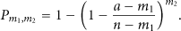
which means that, for a component of order $m_{\mathrm{1}}$ , the circle of acquaintances of this component may consist of $n[\mathrm{1}-(\mathrm{1}-P{)}^{m_{\mathrm{1}}}]$ nodes on average. Let $a=n[\mathrm{1}-(\mathrm{1}-P{)}^{m_{\mathrm{1}}}]$ , the probability $P_{m_{\mathrm{1}},m_{\mathrm{2}}}$ that there is at least one common acquaintance between components $C_A$ and $C_B$ is

$$\begin{array}{cc}& P_{m_{\mathrm{1}},m_{\mathrm{2}}}=\mathrm{1}-{\left(\mathrm{1}-\frac{a-m_{\mathrm{1}}}{n-m_{\mathrm{1}}}\right)}^{m_{\mathrm{2}}}.\end{array}$$

(4)

For example, one may see that, for a network $n=\mathrm{10,000}$ , $m_{\mathrm{1}}=\mathrm{200}$ , and $m_{\mathrm{2}}=\mathrm{1}$ , the probability $P_{m_{\mathrm{1}},m_{\mathrm{2}}}$ tends to 1 when $P>\mathrm{0.02}$ . This provides intuition that, a component of order 200 is attractive and will swallow nodes nearby to form a larger component, a kind of “rich get richer” phenomenon. For two components of order $m_{\mathrm{1}}=m_{\mathrm{2}}=\mathrm{50}$ , the probability $P_{m_{\mathrm{1}},m_{\mathrm{2}}}$ approximates 1 if $P>\mathrm{0.002}$ . In general, the larger the components are, the more likely they are to be mixed together.

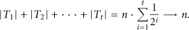
In a random graph $G_{n,N}$ with n vertices and N edges, if $N~cn$ with $c\ge \mathrm{1}/\mathrm{2}$ , the greatest component has (with probability tending to 1 for $n\to +\infty$ ) approximately $n^{\mathrm{2}/\mathrm{3}}$ vertices [10]. As a special case, when $n=\mathrm{10,000}$ , $n^{\mathrm{2}/\mathrm{3}}\approx \mathrm{464}$ , such large component in graph $G_{n,n_{\mathrm{0}}}$ will swallow the whole network with high probability.

Next, we investigate the relationship between the connectivity property of graph $G_{n,n_{\mathrm{0}}}$ and value $n_{\mathrm{0}}$ . To determine the value $n_{\mathrm{0}}$ which will guarantee the connectivity of graph $G_{n,n_{\mathrm{0}}}$ , we employ a well-known algorithm to generate random graphs $G_{n,p}$ with a given degree distribution [11]. Each graph generated has n nodes and $n_{\mathrm{0}}=np$ links per node. The algorithm may lead to a multigraph, either by connecting a node to itself or by connecting two nodes together more than once. However, as n increases, these events become rare and their number becomes statistically insignificant.

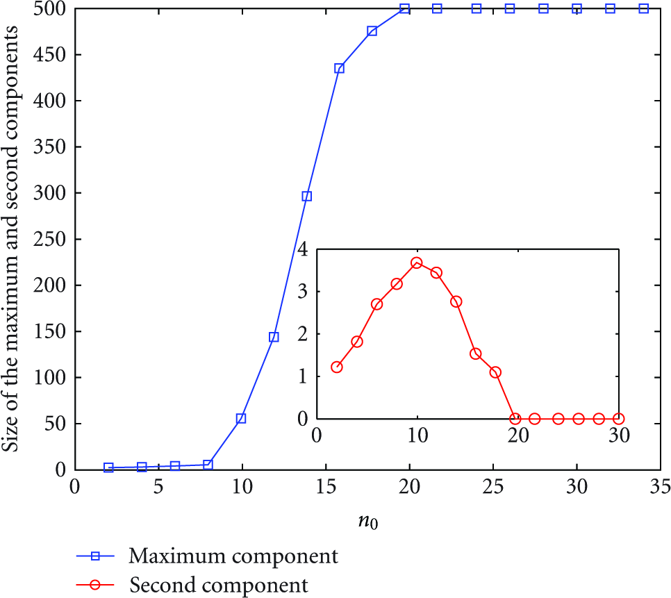
We first generate a random graph with n nodes and $n_{\mathrm{0}}$ links per node, then deploy the nodes into a square region to obtain a random topology. For $n=\mathrm{500}$ , $r=\mathrm{35}\hspace{0.17em}\text{m}$ , and $n_{\mathrm{0}}$ varying, we repeat our simulations 50 times to yield an acceptable confidence of results. For each simulation, we measure empirical values for the maximum component and the second component for each trial, averaged over 50 random topologies. In Figure 3, an interesting phenomenon observed is a “phase transition” as $n_{\mathrm{0}}$ increases. There is a critical value of $n_{\mathrm{0}}$ , above which the graph will almost surely be connected. The maximum component grows rapidly from a component of small size to a giant component when $n_{\mathrm{0}}>\mathrm{10}$ . On the contrary, the size of the second component decreases as $n_{\mathrm{0}}>\mathrm{10}$ .

Figure 3

Size of the maximum and second components in graph $G_{n,n_{\mathrm{0}}}$ for $n=\mathrm{500}$ , $r=\mathrm{35}\hspace{0.17em}\text{m}$ .

Within this context, we want to know, under what conditions is the graph $G_{n,n_{\mathrm{0}}}$ be connected? How can we choose $n_{\mathrm{0}}$ such that the graph $G_{n,n_{\mathrm{0}}}$ constructed by secrecy transfer will be connected with high probability? The answer to this question is crucial in determining the number of acquaintances that an arbitrary node should have initially.

3.1. Lower Bound of Connectivity Threshold

To get a fully connected graph $G_{n,n_{\mathrm{0}}}$ , two conditions must be satisfied. First, the graph $G_{n,r}$ must be connected, which means that, given the value n and a deployment region, the value r should be large enough to guarantee a connected random geometric graph $G_{n,r}$ . Assume n nodes are uniformly deployed in a unit square $[\mathrm{0,1}{]}^{\mathrm{2}}$ , the well-known connectivity threshold $r_c=\sqrt{(\log \hspace{0.17em}\hspace{0.17em}n\pm O(\mathrm{1}))/\pi n}$ [5]. Second, the value $n_{\mathrm{0}}$ must be large enough to get the random graph $G_{n,p}$ fully connected. Consider an arbitrary pair of adjacent nodes A and B in graph $G_{n,n_{\mathrm{0}}}$ which have not established secret key between them. For $G_{n,p}$ is connected, there is at least one path in graph $G_{n,p}$ , say $P_{AB}=A{x}_{\mathrm{0}}{x}_{\mathrm{1}}\cdots x_{k}B$ between nodes A and B. Given any adjacent nodes in path $P_{AB}$ , say $x_i$ and $x_{i+\mathrm{1}}$ , there must exist a path $P\prime =x_i{y}_{\mathrm{1}}{y}_{\mathrm{2}}\cdots y_t{x}_{i+\mathrm{1}}$ from $x_i$ to $x_{i+\mathrm{1}}$ in graph $G_{n,r}$ , for graph $G_{n,r}$ is connected.

For a random graph $G_{n,p}$ , when p is zero, the graph does not have any edge, whereas when p is one, the graph is fully connected. Bolbbás showed that, for monotone properties, there exists a value of p such that the property moves from “nonexistent” to “certainly true” in a very large random graph [1]. The function defining p is called the threshold function of a property. Given a desired probability $P_c$ for graph connectivity, the threshold function p of $G_{n,p}$ is defined by

$$\begin{array}{cc}& P_c=\underset{n\to \infty }{\lim }{P}_r\left[G_{n,p}\text{\hspace{0.17em}is\hspace{0.17em}connected}\right]=e^{e^{-c}},\end{array}$$

(5)

where $p=\ln \hspace{0.17em}(n)/n+c/n$ and c is any real constant.

Therefore, given n we can find p for which the resulting graph $G_{n,p}$ is connected with desired probability $P_c$ . Thus, the lower bound of connectivity threshold of $n_{\mathrm{0}}$ is

$$\begin{array}{cc}& n_{\mathrm{0}}=p\times \left(n-\mathrm{1}\right)=\frac{n-\mathrm{1}}{n}\left[\ln \left(n\right)-\ln \left(-\ln \left(P_c\right)\right)\right].\end{array}$$

(6)

3.2. Analysis Results of Connectivity Threshold

Notice that when $n_{\mathrm{0}}$ is below the lower bound of connectivity threshold mentioned above, the graph $G_{n,p}$ is not connected with high probability, and hence the graph $G_{n,n_{\mathrm{0}}}$ also is not connected with high probability. However, a greater $n_{\mathrm{0}}$ above the lower bound cannot guarantee a connected graph $G_{n,n_{\mathrm{0}}}$ when $n\prime$ is small, where $n\prime$ is the average number of neighbors of a node. For a tighter bound of $n_{\mathrm{0}}$ , correlated with n, $n\prime$ , is not known yet, we only present some analysis results of $n_{\mathrm{0}}$ below.

After the initialization phase of secrecy transfer, we get a random graph. Erdös and Rényi showed that for random graphs, a giant component exists if the average degree of node $〈k〉>\mathrm{1}$ [10]. If $〈k〉<\mathrm{1}$ only small components exist, and the size of the largest component is proportional to $\ln \hspace{0.17em}n$ (n is the number of nodes in the graph). Exactly at the threshold, $〈k〉=\mathrm{1}$ , a component whose size is proportional to $n^{2/3}$ emerges. In the sequel, when $n=\mathrm{10,000}$ , $n\prime =\mathrm{10}$ , and $n_{\mathrm{0}}=\mathrm{200}$ , after the initialization phase of secrecy transfer, the average degree of nodes in the graph $G_{n,n_{\mathrm{0}}}$ , $〈k〉=n^{\prime }(n_{\mathrm{0}}/n)=\mathrm{10}\times (\mathrm{200}/\mathrm{10000})=\mathrm{0.2}$ . In this occasion, the initial graph $G_{n,n_{\mathrm{0}}}$ only consists of small components, such as trees of small size. As the simulation results of initialization phase shown in Figure 2(a), the graph $G_{n,n_{\mathrm{0}}}$ only contains small isolated trees. Our goal is to determine how many such components exist, and the probability that they will be connected to form a giant component.

Let the graph $G_{n,n_{\mathrm{0}}}$ in the initialization phase contains components $C_{\mathrm{1}},C_{\mathrm{2}},\dots ,C_i$ , such that the size of component $C_i$ is $|C_i|={\lambda }_i$ , and ${\lambda }_{\mathrm{1}}\ge {\lambda }_{\mathrm{2}}\ge \cdots \ge {\lambda }_i\ge \mathrm{2}$ . For two components $C_i$ and $C_j$ of order ${\lambda }_i$ and ${\lambda }_j$ , if they are adjacent, the probability that they will be connected through secrecy transfer is

$$\begin{array}{cc}& P_{{\lambda }_{\mathrm{1}},{\lambda }_{\mathrm{2}}}=\mathrm{1}-{\left(\mathrm{1}-\frac{a-{\lambda }_{\mathrm{1}}}{n-{\lambda }_{\mathrm{1}}}\right)}^{{\lambda }_{\mathrm{2}}},\end{array}$$

(7)

where $a=n[\mathrm{1}-{(\mathrm{1}-P)}^{{\lambda }_{\mathrm{1}}}]$ , $P=n_{\mathrm{0}}/n$ .

When secrecy transfer is applied, the graph $G_{n,n_{\mathrm{0}}}$ will evolve continuously. A larger component is more attractive and will swallow nodes nearby to form a larger component with high probability. Popularity is attractive. If a component can absorb nodes nearby by secrecy transfer, it is termed as expandable. Next we estimate the asymptotic probability $P_{\text{expandable}}$ that at least one component in $C_{\mathrm{1}},C_{\mathrm{2}},\dots ,C_i$ is expandable. At first we estimate the number of neighbors $n_{\lambda }^{\prime }$ of a component of size λ.

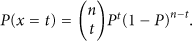
Suppose n nodes distributed uniformly and independently at random in a unit area S, that is, $S=\mathrm{1}$ . Let a component C of size $|C|=\lambda$ lie inside a circle of radius R, $n_{\lambda }^{\prime }$ neighbors of the component C lie outside the circle and be at distance at most r from nodes in the component. Let $S\prime$ be a subarea in the deployment area S, $S\prime \ll S$ . The probability that a node is placed within area $S\prime$ is $P=S\prime /S=S\prime$ . Then, the probability $P(x)$ that of t nodes are placed in the area $S\prime$ is

$$\begin{array}{cc}& P\left(x=t\right)=\left(\begin{array}{c}n\\ t\end{array}\right)P^t{\left(\mathrm{1}-P\right)}^{n-t}.\end{array}$$

(8)

When $n\gg \mathrm{1}$ and $S\prime \ll S$ , we can approximate it with a Poisson distribution,

$$\begin{array}{cc}& P(x=t)\approx \frac{e^{-nP}\cdot {\left(np\right)}^t}{t!}=\frac{e^{-nS\prime }{\left(n{S}^{\prime }\right)}^t}{t!},\end{array}$$

(9)

and the average number of nodes within area $S\prime$ is

$$\begin{array}{cc}& t=nS\prime .\end{array}$$

(10)

In the initial graph $G_{n,n_{\mathrm{0}}}$ , any component of size λ is small ( $\lambda \ll n$ ), and the area $S\prime$ it occupied is also small, that is, $S\prime \ll S=\mathrm{1}$ . Therefore, we have approximately

$$\begin{array}{cc}& \lambda =n\pi R^{\mathrm{2}},\hspace{1em}\hspace{1em}n\prime =n\pi r^{\mathrm{2}}.\end{array}$$

(11)

Thus,

$$\begin{array}{cc}& n_{\lambda }^{\prime }=n\left[{\left(R+r\right)}^{\mathrm{2}}\pi -r^{\mathrm{2}}\pi \right]=n\prime +\mathrm{2}\sqrt{\lambda n\prime }.\end{array}$$

(12)

Therefore, the probability $P_{\lambda }$ that a component of size λ is expandable is

$$\begin{array}{cc}& P_{\lambda }=\mathrm{1}-{\left(\mathrm{1}-P_{\lambda ,\mathrm{1}}\right)}^{n_{\lambda }^{\prime }},\end{array}$$

(13)

where $P_{\lambda ,\mathrm{1}}=(a-\lambda )/(n-\lambda )$ , $a=n[\mathrm{1}-(\mathrm{1}-P{)}^{\lambda }]$ , $P=n_{\mathrm{0}}/n$ .

For a set of components $C_{\mathrm{1}},C_{\mathrm{2}},\dots ,C_i$ , $|C_i|={\lambda }_i$ , the probability $P_{\text{expandable}}$ can be calculated as

$$\begin{array}{ll}& P_{\text{expandable}}\\ \hspace{1em}=\mathrm{1}-\left(\mathrm{1}-P_{{\lambda }_{\mathrm{1}}}\right)\left(\mathrm{1}-P_{{\lambda }_{\mathrm{2}}}\right)\cdots \left(\mathrm{1}-P_{{\lambda }_i}\right)\\ \hspace{1em}=\mathrm{1}-{\left(\mathrm{1}-P_{{\lambda }_{\mathrm{1}},\mathrm{1}}\right)}^{n_{{\lambda }_{\mathrm{1}}}^{\prime }}{\left(\mathrm{1}-P_{{\lambda }_{\mathrm{2}},\mathrm{1}}\right)}^{n_{{\lambda }_{\mathrm{2}}}^{\prime }}\cdots {\left(\mathrm{1}-P_{{\lambda }_i,\mathrm{1}}\right)}^{n_{{\lambda }_{\text{i}}}^{\prime }}\\ \hspace{1em}\approx \mathrm{1}-\exp \left\{-\left(n_{{\lambda }_{\mathrm{1}}}^{\prime }{P}_{{\lambda }_{\mathrm{1}},\mathrm{1}}+n_{{\lambda }_{\mathrm{2}}}^{\prime }{P}_{{\lambda }_{\mathrm{2}},\mathrm{1}}+\dots +{n^{\prime }}_{{\lambda }_i}{P}_{{\lambda }_i,\mathrm{1}}\right)\right\}.\end{array}$$

(14)

Note that for two sets of components $ℂ=\{C_{\mathrm{1}},C_{\mathrm{2}},\dots ,C_i\}$ ( $|C_i|={\lambda }_i$ ) and $ℂ\prime =\{{C\prime }_{\mathrm{1}},{C\prime }_{\mathrm{2}},\dots ,{C\prime }_i\}$ ( $|{C\prime }_i|={\lambda }_i^{\prime }$ ), if ${\lambda }_{\mathrm{1}}\ge {\lambda }_1^{\prime }$ , ${\lambda }_{\mathrm{2}}\ge {\lambda }_2^{\prime }$ , $\dots {\lambda }_i\ge {\lambda }_i^{\prime }$ , then

$$\begin{array}{cc}& n_{{\lambda }_{\mathrm{1}}}^{\prime }\ge n_{{\lambda }_1^{\prime }}^{\prime },\dots ,n_{{\lambda }_{\text{i}}}^{\prime }\ge n_{{\lambda }_i^{\prime }}^{\prime },\\ P_{{\lambda }_{\mathrm{1}},\mathrm{1}}\ge P_{{\lambda }_1^{\prime },\mathrm{1}},\dots ,P_{{\lambda }_i,\mathrm{1}}\ge P_{{\lambda }_i^{\prime },\mathrm{1}}.\end{array}$$

(15)

Therefore, the probability $P_{\text{expandable}}$ that at least one component in set ℂ is expandable is greater than that in set $ℂ\prime$ .

Given parameters n, $n\prime$ , and $n_{\mathrm{0}}$ , after the initialization phase of secrecy transfer, the graph $G_{n,n_{\mathrm{0}}}$ may contain some components $C_{\mathrm{1}},C_{\mathrm{2}},\dots ,C_i$ . The expandable probability of this component set $P_{\text{expandable}}\to \mathrm{1}$ , implies that at least one component in $C_{\mathrm{1}},C_{\mathrm{2}},\dots ,C_i$ is expandable and will grow larger with high probability. Let a component $C_{\mathrm{1}}$ be expandable and become a larger component $C_1^{\prime }$ by swallowing nodes nearby. For $|C_1^{\prime }|>|C_{\mathrm{1}}|$ , the expandable probability $P_{\text{expandable}}^{\prime }$ of components $C_1^{\prime },C_{\mathrm{2}},\dots ,C_i$ is greater than the expandable probability $P_{\text{expandable}}$ of components $C_{\mathrm{1}},C_{\mathrm{2}},\dots ,C_i$ , that is,

$$\begin{array}{cc}& P_{\text{expandable}}^{\prime }>P_{\text{expandable}}⟶\mathrm{1}.\end{array}$$

(16)

Thus, if the expandable probability $P_{\text{expandable}}$ of the initial graph approximates 1, it will become even greater almost surely, and the graph $G_{n,n_{\mathrm{0}}}$ will eventually evolve into a connected graph with high probability if both $G_{n,p}$ and $G_{n,r}$ are connected graphs. However, small expandable probability of the initial graph $G_{n,n_{\mathrm{0}}}$ cannot guarantee a connected graph with high probability and secrecy transfer will terminate with isolated components.

However, exact results of the critical threshold $n_{\mathrm{0}}$ are not known yet, we only present some analysis results below.

In an Erdös-Rényi random graph $G_{n,N}$ with n nodes and N links [10], if $N~l·n^{(k-\mathrm{2})/(k-\mathrm{1})}$ where $l>\mathrm{0}$ , then the number of trees of order k contained in $G_{n,N}$ has in the limit for $n\to +\infty$ a Poisson distribution with mean value

$$\begin{array}{cc}& \stackrel{-}{\lambda }=\frac{{\left(\mathrm{2}l\right)}^{k-\mathrm{1}}{k}^{k-\mathrm{2}}}{k!}.\end{array}$$

(17)

Among these trees, the probability $P_{\text{expandable}}$ that at least one tree of order k is expandable is

$$\begin{array}{cc}& P_{\text{expandable}}=\mathrm{1}-{\left(\mathrm{1}-P_k\right)}^{\stackrel{-}{\lambda }},\end{array}$$

(18)

where $P_k$ is the probability that a tree of order k is expandable, $P_k=\mathrm{1}-{(\mathrm{1}-P_{k,\mathrm{1}})}^{n_k^{\prime }}$ , $n_k^{\prime }=n\prime +\mathrm{2}\sqrt{kn\prime }$ , $P_{k,\mathrm{1}}=(a-k)/(n-k)$ , $a=n[\mathrm{1}-{(\mathrm{1}-n_{\mathrm{0}}/n)}^k]$ , and $\stackrel{-}{\lambda }=(\mathrm{2}l{)}^{k-\mathrm{1}}{k}^{k-\mathrm{2}}/k!$ .

For the graph $G_{n,n_{\mathrm{0}}}$ after the initialization phase of secrecy transfer, the number of links in $G_{n,n_{\mathrm{0}}}$ is

$$\begin{array}{cc}& N=\frac{\mathrm{1}}{\mathrm{2}}n\cdot n\prime P=\frac{\mathrm{1}}{\mathrm{2}}n\cdot n\prime \frac{n_{\mathrm{0}}}{n}=\frac{\mathrm{1}}{\mathrm{2}}n\prime n_{\mathrm{0}}~l\cdot n^{\left(k-\mathrm{2}\right)/\left(k-\mathrm{1}\right)},\end{array}$$

(19)

which yields the result

$$\begin{array}{cc}& k~\mathrm{1}+\frac{\ln n}{\ln \left(2ln/n^{\prime }{n}_0\right)}.\end{array}$$

(20)

Using the above considerations, we can estimate the expandable probability $P_{\text{expandable}}$ of the components (trees) of order k.

We see that, for $n=\mathrm{10,000}$ , $n\prime =\mathrm{10}$ , and $n_{\mathrm{0}}=\mathrm{100}$ , the probability $P_{\text{expandable}}\approx \mathrm{0.6991}$ ; for $n_{\mathrm{0}}=\mathrm{200}$ , the probability $P_{\text{expandable}}\approx \mathrm{1}$ . This indicates that, in this occasion, for $n_{\mathrm{0}}\ge \mathrm{200}$ , the graph $G_{n,n_{\mathrm{0}}}$ will eventually evolve into a connected graph by secrecy transfer with high probability. However, for $n_{\mathrm{0}}<\mathrm{100}$ , the graph $G_{n,n_{\mathrm{0}}}$ may be fragmented and contains no giant component of order n. Furthermore, the critical threshold of $n_{\mathrm{0}}$ is rather sensitive to $n\prime$ . For $n=\mathrm{100,000}$ , $n\prime =\mathrm{30}$ , and $n_{\mathrm{0}}=\mathrm{200}$ , the probability $P_{\text{expandable}}\approx \mathrm{0.9337}$ . If we reduce $n\prime$ to $\mathrm{5}$ , then $P_{\text{expandable}}\approx \mathrm{0.5391}$ . This is because the decline in $n\prime$ will result in the decline in the number of neighbors of a component, so does the expandable probability.

On the other hand, the probability $P_{\mathrm{0}}$ that secrecy transfer cannot take place after the initialization phase is

$$\begin{array}{cc}& P_{\mathrm{0}}={\left[{\left(\mathrm{1}-\frac{n_{\mathrm{0}}}{n}\right)}^{n^{\prime }}\right]}^n={\left(\mathrm{1}-\frac{n_{\mathrm{0}}}{n}\right)}^{n\cdot n\prime }\approx e^{-n_{\mathrm{0}}\cdot n\prime },\end{array}$$

(21)

which is only dependent on $n_{\mathrm{0}}$ and $n\prime$ . Less $n_{\mathrm{0}}$ or $n\prime$ , higher the probability $P_{\mathrm{0}}$ .

4. Heterogeneous Network

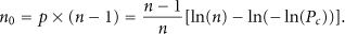
Consider graph $G_{n,r}$ of n nodes with $n_{\mathrm{0}}$ acquaintances per node randomly selected among the nodes in the graph, we are also interested in the number of rounds needed for secrecy transfer to reach a stable state. It is shown in Section 3 that a necessary condition for graph $G_{n,n_{\mathrm{0}}}$ to be connected is that graphs $G_{n,p}$ and $G_{n,r}$ must be fully connected. However, the speed of the convergence of secrecy transfer depends on the values of $n_{\mathrm{0}}$ , r for given n. To gain insight, we first consider the value r and perform a simulation-based study of it. Employing a uniform random generator, we position $n=500$ nodes in a square planar region of $\mathrm{500}\times \mathrm{500}\hspace{0.17em}{\text{m}}^{\mathrm{2}}$ , following our deployment from Section 3. For each random topology, we estimate the speed of the convergence of secrecy transfer as the number of rounds that it needs to perform to reach its stable state. At each round, each pair of adjacent nodes in the graph $G_{n,n_{\mathrm{0}}}$ employ secrecy transfer to try to get connected. If there is no new edge is added in this round, secrecy transfer reaches its stable state and terminates. We observe from Figure 4 that, as the value r increases, the stable state is reached with a faster speed, and for value $n_{\mathrm{0}}$ , the number of rounds reaches its peak when $n_{\mathrm{0}}$ approximates to its connectivity threshold.

Figure 4

Value $n_{\mathrm{0}}$ versus. number of rounds of secrecy transfer for various values of the radius r.

Conventionally, a wireless network consists of some nodes as supernodes with greater communication radius than normal nodes. The use of these supernodes lead to important characteristics of complex networks [12]: a small average shortest path length between all nodes, and a high-cluster coefficient, which help us saving network resources, avoiding excessive communication, and reducing the time to data delivery. Figure 5 depicts plots of secrecy transfer with $n=\mathrm{500}$ nodes deployed over a $\mathrm{500}\times \mathrm{500}\hspace{0.17em}{\text{m}}^{\mathrm{2}}$ field, $n_{\mathrm{0}}=\mathrm{20}$ , and $r=\mathrm{35}\hspace{0.17em}\text{m}$ , among them there are 25 supernodes (squares in the figures) with a larger communication radius $R=\mathrm{150}\hspace{0.17em}\text{m}$ and only bidirectional links are considered.

Figure 5

Secrecy transfer process in a heterogeneous network, $n=\mathrm{500}$ , $s=\mathrm{25}$ , $r=\mathrm{35}\hspace{0.17em}\text{m}$ , and $R=\mathrm{150}\hspace{0.17em}\text{m}$ .

From the simulation results illustrated in Figure 6, we conclude that, compared to the homogeneous network case, for a heterogeneous network with supernodes, as the radius R of supernodes grows, the value of $n_{\mathrm{0}}$ required to maintain connectivity of graph $G_{n,n_{\mathrm{0}}}$ decreases, the speed of the convergence of secrecy transfer accelerates. Hierarchically, supernodes can form a higher layer, while normal nodes constitute a lower layer of the network. An implication of a heterogeneous network is that it has better performance with regard to improving energy, power and topology control, scalability, and fault-tolerance and routing efficiency.

Figure 6

The maximum component and rounds of secrecy transfer in heterogeneous networks.

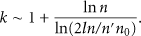
One of the most important properties of a network is the degree distribution, or the fraction $P(k)$ of nodes having k connections (degree k). Although the degree distribution alone is not enough to characterize the network, it has great influence on the network's structure and behavior. A well-known result for Erdös-Rényi random graph is that the degree distribution is Poissonian, $P(k)=e^{-\lambda }{\lambda }^k/k!$ , where $\lambda =〈k〉$ is the average degree. For many real networks, such as the Internet, WWW, citations of scientific articles, airline networks, and many more, they often exhibit a scale-free degree distribution, $P(k)=C{k}^{-\gamma }$ , $k=m,\dots ,K$ , where $C\approx (\gamma -\mathrm{1})m^{\gamma -\mathrm{1}}$ is a normalization faction, and m and K are the lower and upper cutoffs for the degree of a node, respectively. A scale-free network with $\mathrm{2}<\gamma <\mathrm{3}$ and N nodes have diameter $d~\ln \hspace{0.17em}\hspace{0.17em}\ln \hspace{0.17em}\hspace{0.17em}N$ and can be considered as “ultra small-world” network. In fact, the diameter of network is relevant in many fields regarding communication and computer networks, such as routing, searching, and transport of information. All these processes become more efficient when the diameter is smaller.

Intuitively, compared to homogeneous networks, a heterogeneous network with supernodes has a degree distribution different from Poisson distribution. Next, we discuss the degree distribution of heterogeneous networks. Let n nodes and s supernodes be distributed uniformly and independently at random in a square of area 1, $[\mathrm{0,1}{]}^{\mathrm{2}}$ , the communication radii of nodes and supernodes are r and R ( $r<R$ ), respectively, and only bidirectional links are taken into considerations.

For a heterogeneous network, there are two degree distributions, one for each type of nodes. For normal nodes with radii r, the degree distribution $P_n(k)$ is Poissonian,

$$\begin{array}{cc}& P_n\left(k\right)=\frac{e^{-{\lambda }_n}{{\lambda }_n}^k}{k!},\hspace{1em}\text{where}\hspace{0.17em}{\lambda }_n=〈k〉=\pi \left(n+s\right)r^{\mathrm{2}},\end{array}$$

(22)

whereas the degree distribution of supernodes is

$$\begin{array}{cc}& P_s\left(k\right)=\frac{e^{-{\lambda }_s}{{\lambda }_s}^k}{k!},\hspace{1em}\text{where}\hspace{0.17em}{\lambda }_s=〈k〉=\pi \left(n{r}^{\mathrm{2}}+s{R}^{\mathrm{2}}\right).\end{array}$$

(23)

Therefore, the degree distribution $P_{\mathrm{2}-h}(k)$ of the heterogeneous network is

$$\begin{array}{cc}& P_{\mathrm{2}-h}\left(k\right)=\frac{n}{n+s}{P}_n\left(k\right)+\frac{s}{n+s}{P}_s\left(k\right).\end{array}$$

(24)

From the degree distribution $P_{\mathrm{2}-h}(k)$ derived above, we depict and compare it with two different networks. In Figure 7(a) we show the degree distribution of a heterogeneous network with $n=\mathrm{9,000}$ , $s=\mathrm{1,000}$ , $r=\mathrm{0.01}$ , and $R=\mathrm{0.1}$ . In Figure 7(b), we compare $P_{\mathrm{2}-h}(k)$ with power law $P(k)=k^{-\mathrm{2}}$ and Poisson distribution $P(k)={\lambda }^k{e}^{-\lambda }/k!$ , where $\lambda =(n+s)\pi r^{\mathrm{2}}$ . As the figures shown, the degree distribution of a heterogeneous network with two peaks is different from a Poisson distribution and right-skewed to a power law. The results imply that the behavior of a heterogeneous network has some characteristics of scale-free network, such as small diameter.

Figure 7

Degree distributions for different networks. The horizontal axis is node degree k (or $\log \hspace{0.17em}k$ ), and the vertical axis is the probability distribution $P(k)$ (or $\log \hspace{0.17em}P(k)$ ) of degrees, that is, the fraction of nodes that have degree greater than or equal to k. The network shown in (a) is a heterogeneous network with two types of nodes, three networks (of power law, heterogeneous, and Poisson distribution) are depicted in (b) with a logarithmic degree scale.

Now consider the placement of nodes with more types. Suppose that the network contains t types of nodes, denoted as $T_{\mathrm{1}},T_{\mathrm{2}},\dots ,T_t$ . For nodes of type $T_i$ , the number of nodes $|T_i|$ in it and node's communication radius $r_i$ satisfy the conditions,

$$\begin{array}{cc}& r_{\mathrm{1}}<r_{\mathrm{2}}<\cdots <r_t,\\ \left|T_{\mathrm{1}}\right|>\left|T_{\mathrm{2}}\right|>\cdots >\left|T_t\right|.\end{array}$$

(25)

For simplicity, let n denote the total number of nodes in the network, and

$$\begin{array}{cc}& \left|T_{\mathrm{1}}\right|=\frac{n}{\mathrm{2}},\hspace{1em}\hspace{1em}\left|T_{\mathrm{2}}\right|=\frac{n}{{\mathrm{2}}^{\mathrm{2}}},\dots ,\hspace{1em}\left|T_t\right|=\frac{n}{{\mathrm{2}}^t}.\end{array}$$

(26)

It is clear that when $n\to +\infty$ and $t\to +\infty$ ,

$$\begin{array}{cc}& \left|T_{\mathrm{1}}\right|+\left|T_{\mathrm{2}}\right|+\cdots +\left|T_t\right|=n\cdot \sum _{i=1}^t\frac{\mathrm{1}}{{\mathrm{2}}^i}⟶n.\end{array}$$

(27)

Recall that the degree of each type of nodes has a Poisson distribution with different mean value. To derive the degree distribution $P_{t-h}(k)$ of the network, we first determine the degree distribution $P_i(k)$ of nodes of type $T_i$ ,

$$\begin{array}{cc}& P_i\left(k\right)=\frac{e^{-{\lambda }_i}{\lambda }_i^k}{k!},\hspace{1em}\left(i=\mathrm{1},\dots ,t\right),\end{array}$$

(28)

where,

$$\begin{array}{ll}& {\lambda }_{\mathrm{1}}=\pi r_{\mathrm{1}}^{\mathrm{2}}n,\\ {\lambda }_{\mathrm{2}}=\pi \frac{r_{\mathrm{1}}^{\mathrm{2}}+r_{\mathrm{2}}^{\mathrm{2}}}{\mathrm{2}}n,\\ {\lambda }_{\mathrm{3}}=\pi \frac{\mathrm{2}{r}_{\mathrm{1}}^{\mathrm{2}}+r_{\mathrm{2}}^{\mathrm{2}}+r_{\mathrm{3}}^{\mathrm{2}}}{\mathrm{4}}n,\\ {\lambda }_{\mathrm{4}}=\pi \frac{\mathrm{4}{r}_{\mathrm{1}}^{\mathrm{2}}+\mathrm{2}{r}_{\mathrm{2}}^{\mathrm{2}}+r_{\mathrm{3}}^{\mathrm{2}}+r_{\mathrm{4}}^{\mathrm{2}}}{\mathrm{8}}n,\\ {\lambda }_{\mathrm{5}}=\pi \frac{\mathrm{8}{r}_{\mathrm{1}}^{\mathrm{2}}+\mathrm{4}{r}_{\mathrm{2}}^{\mathrm{2}}+\mathrm{2}{r}_{\mathrm{3}}^{\mathrm{2}}+r_{\mathrm{4}}^{\mathrm{2}}+r_{\mathrm{5}}^{\mathrm{2}}}{\mathrm{16}}n,\\ \hspace{1em}\cdots \cdots .\end{array}$$

(29)

Therefore, the degree distribution of the heterogeneous network with t types of nodes is

$$\begin{array}{ll}& P_{t-h}\left(k\right)=\frac{\mathrm{1}}{\mathrm{2}}{P}_{\mathrm{1}}\left(k\right)+\frac{\mathrm{1}}{\mathrm{4}}{P}_{\mathrm{2}}\left(k\right)+\cdots +\frac{\mathrm{1}}{{\mathrm{2}}^t}{P}_t\left(k\right)\\ =\frac{\mathrm{1}}{k!}(\frac{\mathrm{1}}{\mathrm{2}}{e}^{-{\lambda }_{\mathrm{1}}}{\lambda }_{\mathrm{1}}^k+\frac{\mathrm{1}}{\mathrm{4}}{e}^{-{\lambda }_{\mathrm{2}}}{\lambda }_{\mathrm{2}}^k+\cdots +\frac{\mathrm{1}}{{\mathrm{2}}^t}{e}^{-{\lambda }_t}{\lambda }_t^k).\end{array}$$

(30)

For $P_{t-h}(k)$ is complicated, we present some numerical results on it. Figure 8 shows the degree distribution $P_{t-h}(k)$ for $r_{\mathrm{1}}=\mathrm{0.01}$ , $r_{\mathrm{2}}=\mathrm{0.03}$ , $r_{\mathrm{3}}=\mathrm{0.05}$ , $r_{\mathrm{4}}=\mathrm{0.07}$ , $r_{\mathrm{5}}=\mathrm{0.09}$ , $r_{\mathrm{6}}=\mathrm{0.11}$ , $r_{\mathrm{7}}=\mathrm{0.13}$ , and $r_{\mathrm{8}}=\mathrm{0.2}$ . As expected, the degree distribution of the heterogeneous network approaches power law $P(k)\propto k^{-\mathrm{2}}$ . This implies that heterogeneous network maintains some statistical properties of a scale-free network. Therefore, it is plausible that the convergence speed of secrecy transfer in a heterogeneous network is faster than that in a homogeneous network.

Figure 8

Degree distributions.

5. Implementation of Secrecy Transfer

In this section, we elaborate the implementation method of secrecy transfer. The method contains three phases: the initialization phase, the secrecy transfer phase, and the update phase. To implement secrecy transfer efficiently, we use Bloom Filter [13] for membership queries.

Bloom Filter

A Bloom Filter is a popular data structure used for membership queries. It represents a set $S=[s_{\mathrm{1}},\dots ,s_n]$ using k independent hash functions $h_{\mathrm{1}},\dots ,h_k$ and a string of m bits, each of which is initially set to 0. For each $s\in S$ , we hash it with all the k hash functions and obtain their values $h_i(s)$ ( $\mathrm{1}\le i\le k$ ). The bits corresponding to these values are then set to 1 in the string. To determine whether an item $s\prime$ is in S, bits $h_i(s\prime )$ are checked. If all these bits are 1s, $s\prime$ is considered to be in S.

Since multiple hash values may map to the same bit, Bloom Filter may yield false positives. That is, an element is not in S but its bits $h_i(s)$ are collectively marked by elements in S. If the hash is uniformly random over m values, the probability that a bit is 0 after all the n elements are hashed and their bits marked is $(\mathrm{1}-\mathrm{1}/m{)}^{kn}\approx e^{-kn/m}$ . Therefore, the probability for a false positive is $(\mathrm{1}-(\mathrm{1}-\mathrm{1}/m{)}^{kn}{)}^k\approx (\mathrm{1}-e^{-kn/m}{)}^k$ . The right hand side is minimized when $k=(m/n)\hspace{0.17em}\ln \hspace{0.17em}\mathrm{2}$ in which case it becomes $(\mathrm{1}/\mathrm{2}{)}^k=(\mathrm{0.6185}{)}^{m/n}$ .

5.1. Initialization Phase

We first generate a random graph with n nodes and $n_{\mathrm{0}}$ links per node. For each link a secret key is assigned to it. Each node stores the ID of its neighbors and the corresponding secret key between them. For instance, if node i has $n_{\mathrm{0}}$ neighbors $i_{\mathrm{1}},\dots ,i_{n_{\mathrm{0}}}$ , it constructs an acquaintanceship set

$$\begin{array}{cc}& A_i=\left\{\left(i_{\mathrm{1}},K_{i,i_{\mathrm{1}}}\right),\dots ,\left(i_{n_{\mathrm{0}}},K_{i,i_{n_{\mathrm{0}}}}\right)\right\},\end{array}$$

(31)

where $K_{i,i_{\mathrm{1}}}$ is the assigned secret key between node i and its neighbor $i_{\mathrm{1}}$ .

After that nodes are deployed randomly over a field.

5.2. Secrecy Transfer Phase

Suppose two adjacent components, $C_A$ and $C_B$ , have, respectively, $m_{\mathrm{1}}$ and $m_{\mathrm{2}}$ nodes, nodes $A\in C_A$ and $B\in C_B$ are adjacent. For component $C_A$ , a component head (at first after initialization phase, each node is a component head of its own since all nodes are isolated. After several rounds of secrecy transfer process, some large components emerge. To reduce the communication cost, a node is selected to be a component head according to its centrality in the component. To simply the procedure, the node with the highest degree is chosen to be the component head) is selected. He stores all the ID of nodes belonging to the component $C_A$ in a component member set

$$\begin{array}{cc}& \text{C}{\text{M}}_{C_A}=\left\{a_{\mathrm{1}},\dots ,a_{m_{\mathrm{1}}}\right\},\end{array}$$

(32)

where $a_i\in C_A$ .

Each node stores a Bloom Filter ${\text{BF}}_{C_A}$ which contains all the nodes in the acquaintance circle of $C_A$ . That is, the nodes in $C_A$ and the acquaintances of node i for all $i\in C_A$ . If an adjacent node k is added to $C_A$ , the Bloom Filter ${\text{BF}}_k$ of node k is inserted into ${\text{BF}}_{C_A}$ , that is, a new Bloom Filter ${\text{BF}}_{C_A^{\prime }}$ for the new component $C_A^{\prime }=C_A+k$ is created, that is, ${\text{BF}}_{C_A^{\prime }}={\text{BF}}_{C_A}+{\text{BF}}_k$ .

If two components $C_A$ and $C_B$ get connected and melt into a larger component $C_{AB}$ , a new Bloom Filter of component $C_{AB}$ , ${\text{BF}}_{C_{AB}}={\text{BF}}_{C_A}+{\text{BF}}_{C_B}$ , is created and stored in nodes of $C_{AB}$ . To further improve the performance, not all nodes in $C_A$ or $C_B$ need to update its ${\text{BF}}_{C_A}$ or ${\text{BF}}_{C_B}$ to ${\text{BF}}_{C_{AB}}$ , only nodes whose neighbors are not all connected to them need to store the updated Bloom Filter ${\text{BF}}_{C_{AB}}$ of the new component $C_{AB}$ . As depicted in Figure 9, $C_A$ and $C_B$ melt into a larger component $C_{AB}$ , an isolated node E is adjacent to nodes A, B, F, and G. After $C_A$ and $C_B$ get connected, only nodes A, B, F, and G in $C_{AB}$ have unconnected neighbor. Therefore, they need to store the new ${\text{BF}}_{C_{AB}}$ and will broadcast it later.

Figure 9

Secrecy transfer phase.

Next, we give an overview of the operations of secrecy transfer. In general, the operation of secrecy transfer is initiated by a new created component. Let $C_A$ be a new component that has “swallowed” node H, nodes A and F have already updated their ${\text{BF}}_{C_A}$ (to insert the ID of node H into it), and let $C_B$ be an adjacent component of $C_A$ . After that, nodes A and F broadcast ${\text{BF}}_{C_A}$ to their adjacent nodes B and E. On receiving the ${\text{BF}}_{C_A}$ from component $C_A$ , node B sends a query message containing ${\text{BF}}_{C_A}$ to the component head of $C_B$ , say node I, where the component member set of $C_B$ , $\text{C}{\text{M}}_{C_B}=\{b_{\mathrm{1}},\dots ,b_{m_{\mathrm{2}}}\}$ , is stored. The component head I then determines whether the nodes in set $\text{C}{\text{M}}_{C_B}$ are in the Bloom Filter ${\text{BF}}_{C_A}$ . If a node, say $D\in \text{C}{\text{M}}_{C_B}$ , is found in the Bloom Filter ${\text{BF}}_{C_A}$ , node I answers node B by sending D to it. Node B then tells A that there is a node $D\in C_B$ belonging to the acquaintance circle of component $C_A$ . After that, nodes A broadcasts a query message with the ID of node D in component $C_A$ . Each node in $C_A$ verifies whether node D belongs to its acquaintanceship set. As illustrated in Figure 9, if the acquaintanceship set of node $C\in C_A$ contains node D, that is, $A_C=\{\dots ,(D,K_{CD}),\dots \}$ , the node C transmits a response message (C, D) to node A. After obtaining the acquaintance node pair (C, D) from C, node A knows that nodes $C\in C_A$ and $D\in C_B$ are acquaint with each other (they have a shared key $K_{CD}$ ). Now nodes A and B can establish a secret key $K_{AB}$ as mentioned in Section 2.

5.3. Updated Phase

After the secret key $K_{AB}$ between nodes A and B is established, two components become a larger component $C_{AB}$ , we then should update the acquaintance circle of $C_{AB}$ for nodes who have unconnected neighbors. A new component head is also need to be selected according to the degree distribution of nodes in $C_{AB}$ . As to the network in Figure 9, if node I is the new component head of $C_{AB}$ , the component member set is updated to be

$$\begin{array}{cc}& \text{C}{\text{M}}_{A_B}=\text{C}{\text{M}}_{C_A}+\text{C}{\text{M}}_{C_B}=\left\{a_{\mathrm{1}},\dots ,a_{m_{\mathrm{1}}},b_{\mathrm{1}},\dots ,b_{m_{\mathrm{2}}}\right\}.\end{array}$$

(33)

Finally, if nodes have updated their Bloom Filter ${\text{BF}}_{C_{AB}}$ , they broadcast the new ${\text{BF}}_{C_{AB}}$ to their neighbors to find chances for new links. Recursively, this procedure is applied until there is no node has updated its Bloom Filter.

5.4. Security Analysis

As discussed in Section 2, secrecy transfer is robust against eavesdrop attack, for each edge is added via the existing trustiness between nodes. In this subsection, we study the resilience of secrecy transfer against the node compromise attack. Let $n_c$ denote the number of nodes that have been captured. Suppose the compromised nodes are independently and random distributed among the entire deployment region.

Theoretically, as depicted in Figure 9, if any node in the paths $A-F-C$ and $D-I-B$ is compromised, the key $K_{AB}$ between nodes A and B is not secure. Suppose that the length of two paths are $l_{\mathrm{1}}$ and $l_{\mathrm{2}}$ , respectively. It is easy to estimate the probability that a new established key $K_{AB}$ is compromised as the following:

$$\begin{array}{cc}& P\left\{K_{AB}\hspace{0.17em}\text{is}\hspace{0.17em}\text{compromised}\right\}=\mathrm{1}-\frac{\left(\begin{array}{c}{l}_{\mathrm{1}}+l_{\mathrm{2}}\\ n-n_c\end{array}\right)}{\left(\begin{array}{c}{l}_{\mathrm{1}}+l_{\mathrm{2}}\\ n\end{array}\right)},\end{array}$$

(34)

where n is the number of node in the network.

Unfortunately, even if all nodes in two paths are not compromised, the key $K_{AB}$ may be unsecure. For instance, let a path from A to C be $A-H_{\mathrm{1}}-H_{\mathrm{2}}-H_{\mathrm{3}}-H_{\mathrm{4}}-C$ , and all nodes in the path have not been compromised. Node A sends $K_{AB}$ to $H_{\mathrm{1}}$ by sending ${\{K_{AB}\}}_{K_{A{H}_{\mathrm{1}}}}$ , $H_{\mathrm{1}}$ then transmits $\{K_{AB}{\}}_{K_{H_{\mathrm{1}}{H}_{\mathrm{2}}}}$ to node $H_{\mathrm{2}}$ until $K_{AB}$ reaches the last node C. If $K_{A{H}_{\mathrm{1}}},K_{H_{\mathrm{1}}{H}_{\mathrm{2}}},\dots ,K_{H_{\mathrm{4}}C}$ are not compromised, $K_{AB}$ is still secure after it is transmitted across the path. However, if a key, such as $K_{H_{\mathrm{1}}{H}_{\mathrm{2}}}$ , is compromised, an adversary may eavesdrop on the communication flows between nodes $H_{\mathrm{1}}$ and $H_{\mathrm{2}}$ to obtain $\{K_{AB}{\}}_{K_{H_{\mathrm{1}}{H}_{\mathrm{2}}}}$ , thus $K_{AB}$ is leaked.

In general, if there are compromised nodes in the network, any key established by secrecy transfer between two neighbors $H_{\mathrm{1}}$ and $H_{\mathrm{2}}$ may be unsecure unless nodes $H_{\mathrm{1}}$ and $H_{\mathrm{2}}$ are acquaint with each other initially. For any pair of acquaintance nodes, the secret key between them is preloaded before the network is deployed and is considered unbreakable (unless the node is compromised). As to any key established by secrecy transfer, compromised nodes may degrade its security since lots of nodes are involved in the process of the negotiation of a new link key.

In order to set up a more secure channel between nodes A and C, it is reasonable to use the acquaintanceship set of nodes. Suppose in a path $A-H_{\mathrm{1}}-H_{\mathrm{2}}-H_{\mathrm{3}}-H_{\mathrm{4}}-C$ , (A, $H_{\mathrm{3}}$ ), ( $H_{\mathrm{1}}$ , $H_{\mathrm{3}}$ ), and ( $H_{\mathrm{1}}$ , C) are three pair of acquaintances. To send a secret key $K_{AB}$ to C, node A can send $\{K_{AB}{\}}_{K_{A{H}_{\mathrm{3}}}}$ to $H_{\mathrm{3}}$ , $H_{\mathrm{3}}$ then sends $\{K_{AB}{\}}_{K_{H_{\mathrm{1}}{H}_{\mathrm{3}}}}$ to $H_{\mathrm{1}}$ . At last, node C can get $\{K_{AB}{\}}_{K_{H_{\mathrm{1}}C}}$ from $H_{\mathrm{1}}$ . The advantage of this method is that all communications are encrypted with predistributed keys. If nodes A, C, $H_{\mathrm{1}}$ , and $H_{\mathrm{3}}$ are not compromised, the key $K_{AB}$ is secure after the transmission. However, such a secure logical path in a set of nodes may not exist. For a path of l nodes, their initial acquaintanceship can be viewed as a random graph ${\widehat{G}}_{n,p}$ , where $n=l$ and $p=n_{\mathrm{0}}/n$ . If ${\widehat{G}}_{n,p}$ is connected, a logical path exists.

If an adversary is not present at the network before secrecy transfer has completed, or it takes more time than a secure interval to compromise nodes, the communication links established by secrecy transfer are secure; otherwise, undetected malicious nodes may degrade the security of secrecy transfer and jeopardize the network. In [14], authors investigated the potentially disastrous threat of node compromise spreading (via communication and preestablished mutual trust) in wireless sensor networks and proposed an epidemiological model to investigate the probability of a breakout. This model can be adapted to analyze the spread of malicious behavior of compromised nodes in the process of secrecy transfer. But how to design efficient countermeasures is still unknown.

5.5. Storage Overhead

A node, say i, needs to store

• (1)

an acquaintanceship set

$$\begin{array}{cc}& A_i=\left\{\left(i_{\mathrm{1}},K_{i,i_{\mathrm{1}}}\right),\left(i_{\mathrm{2}},K_{i,i_{\mathrm{2}}}\right),\dots ,\left(i_{n_{\mathrm{0}}},K_{i,i_{n_{\mathrm{0}}}}\right)\right\},\end{array}$$

(35)

where $i_{\mathrm{1}},i_{\mathrm{2}},\dots ,i_{n_{\mathrm{0}}}$ are the acquaintances of node i, $K_{i,i_{\mathrm{1}}},K_{i,i_{\mathrm{2}}},\dots ,K_{i,i_{n_{\mathrm{0}}}}$ are the corresponding secret keys with each acquaintance, respectively.

(2)

$n\prime$ secret keys established with its neighbors,

(3)

a Bloom Filter $\text{B}{\text{F}}_{C_A}$ ( $i\in C_A$ ).

For a component head j ( $j\in C_A$ ), in addition to the secret values a normal node stores, it also stores a component member set

$$\begin{array}{cc}& \text{C}{\text{M}}_{C_A}=\left\{a_{\mathrm{1}},\dots ,a_m\right\},\end{array}$$

(36)

where $a_{\mathrm{1}},\dots ,a_m$ are the members of component $C_A$ , m is the cardinality of the component.

6. Applications of Secrecy Transfer

The need for untethered distributed communications and computing continues to drive advances in mobile communications and wireless networking. To serve this purpose, wireless sensor networks have been envisioned to consist of groups of lightweight sensor nodes that may be randomly and densely deployed to observe data within a physical region of interest [15].

In many applications, such as target tracking, battlefield surveillance, and intruder detection, sensor networks are often deployed in hostile environments. To protect the sensitive data, secret keys should be established to achieve data confidentially, integrity, and authentication between communicating parties [16–19]. The first practical key predistribution scheme for sensor network is random key predistribution scheme introduced by Eschenauer and Gligor [7]. Its operation can be briefly described as follows. A random pool S of keys is selected from the key space. Each sensor node receives a random subset of m keys (key ring) from the key pool before deployment. Any two nodes able to find one common key within their respective subsets can use that key as their shared secret to initiate communication. Moreover, the network can be viewed as a random graph $G_{n,p}$ , each edge added if two adjacent nodes can find one common key within their key rings. A major advantage of this scheme is the exclusion of base stations in key management, but a fixed number of compromised sensors causes a fraction of the remaining network to become insecure. Successive sensor captures enable the adversary to reveal network key pool and use them to attack other sensors. In addition, the storage overhead is still high for lightweight sensor nodes. As mentioned previously, secrecy transfer can turn a random graph to a secure random geometric graph. If secrecy transfer is applied with the random key predistribution scheme, the storage overhead of nodes is lower and it can achieve better resilience against node capture attack.

In [20], an asymmetric key predistribution scheme AKPS for sensor networks was proposed. Each nodes only store two secret values initially, a large amount of storage is shifted to keying material servers (KMS). Since AKPS needs to provide public keying material for any pair of nodes, a KMS should store $\left(\begin{array}{c}n\\ 2\end{array}\right)$ public keying material for a network of n nodes. Roughly speaking, AKPS is not viable for arbitrary large network. We find that, if secrecy transfer is used, a KMS does not need to be preloaded with $\left(\begin{array}{c}n\\ 2\end{array}\right)$ public keying material. Specially, suppose $n^{*}$ out of $\left(\begin{array}{c}n\\ 2\end{array}\right)$ public keying material are randomly picked, the initial probability that two arbitrary sensors can establish a secret key is $p=n^{*}/\left(\begin{array}{c}n\\ 2\end{array}\right)=\mathrm{2}{n}^{*}/n(n-\mathrm{1})$ , which means that, any nodes has $n_{\mathrm{0}}=n\times p=\mathrm{2}{n}^{*}/(n-\mathrm{1})$ “acquaintances” on average. As before, if $n_{\mathrm{0}}$ is larger than the connectivity threshold, we can repeat the construction process of secrecy transfer to get a connected graph $G_{n,n_{\mathrm{0}}}$ which will guarantee that any pair of adjacent nodes can establish secret keys.

7. Conclusion

This work presented a secrecy transfer algorithm which is directly based on the idea that networks form primarily by people introducing pairs of their acquaintances to one another. The resulting network, showing both properties of random graph and random geometric graph, cannot only model the introduction process in social networks, but also be used to protect the network.