Mobile Sensor Waypoint Navigation via RF-Based Angle of Arrival Localization

Abstract

Over the past decade, wireless sensor networks have advanced in terms of hardware design, communication protocols, and resource efficiency. Recently, there has been growing interest in mobility, and several small-profile sensing devices that control their own movement have been developed. Unfortunately, resource constraints inhibit the use of traditional navigation methods because these typically require bulky, expensive sensors, substantial memory, and a generous power supply. Therefore, alternative navigation techniques are required. In this paper, we present a navigation system implemented entirely on resource-constrained sensors. Localization is realized using triangulation in conjunction with radio interferometric angle-of-arrival estimation. A digital compass is employed to keep the mobile node on the desired trajectory. We also present a variation of the approach that uses a Kalman filter to estimate heading without using the compass. We demonstrate that a resource-constrained mobile sensor can accurately perform waypoint navigation with an average position error of 0.95 m.

1. Introduction

Typically, autonomous navigation is performed by robots equipped with cameras, laser rangefinders, sonar arrays, and other sophisticated sensors for collecting range and bearing information. These sensor data are then used to compute spatial relationships such as position and proximity, which enable the robot to follow a given trajectory. However, these sensors are large, expensive, have considerable power requirements, and/or require a powerful computing platform to analyze sensor data. In recent years, mote-sized mobile sensor platforms have been developed, that are unable to use traditional navigation methods because of their small size and limited resources [1–5]. This emerging class of mobile sensor would greatly benefit from navigation techniques geared towards resource-constrained devices.

In order to enable navigation in mobile wireless sensor networks (MWSNs), we must develop new methods for estimating position and deriving motion vectors that are rapid and accurate in spite of the limited resources available. Localization in wireless sensor networks has been studied extensively, and several techniques exist that provide submeter accuracy. However, these techniques are often unacceptable for mobile sensor localization due to algorithm complexity and cost. For example, although GPS receivers are available for mote-scale devices, they are still relatively expensive [6]. The Cricket location-support system requires customized hardware with ultrasonic sensors [7]. Other techniques such as the radio interferometric positioning system (RIPS) do not require additional hardware support; however, localization latency is prohibitively high for mobile devices [8].

In this paper, we propose a localization and waypoint navigation system called TripNav, in which a mobile sensor node follows a path by navigating between position coordinates. Position estimates are obtained using a localization technique we developed that combines radio interferometric angle-of-arrival estimation [9] with least squares triangulation [10]. We use this approach because it provides rapid and accurate position estimates and runs on resource-constrained sensor nodes without the need for hardware modifications. These properties are desirable because they enable such a system to be assembled and deployed quickly and inexpensively using commercial off-the-shelf (COTS) components.

Way-finding represents a major category of navigational behavior [11]. Simple waypoint navigation scenarios include automated transportation routes and sentries that patrol a path along the perimeter of a secure area. For our research, the mobile sensor node is provided with a target speed and a set of waypoints and is instructed to pass by each waypoint in the order they are given. The node is comprised of an XSM mote [12] mounted to an iRobot Create [13]. The Create is a programmable robot that hosts a small suite of sensors; however, we use it only as a mobile platform, and all localization and navigation control operations are performed on the attached mote. In addition, we employ a digital compass for estimating heading, from which we can calculate the heading error of the mobile sensor with respect to the desired trajectory. An alternate method is also presented, in which the digital compass is not required, and heading is estimated using an extended Kalman filter (EKF). A simple controller, implemented in software, is then used to derive the necessary wheel speeds for maintaining the correct heading.

In previous work [9], we presented a system for estimating the angle-of-arrival of an interference signal. The system is comprised entirely of COTS sensor nodes, it is completely distributed, bearing can be estimated rapidly, and no additional hardware is required. Our present research builds on this technique by estimating bearing to multiple anchors and then determining position using triangulation. Because the technique is rapid, it is appropriate for mobile devices, which must continuously update their position estimates for navigation. By implementing our angle-of-arrival technique on a mobile platform and using a simple waypoint navigation approach for determining motion vectors, we are able to satisfy the main criteria for a successful MWSN [14]. These criteria include (1) no hardware modifications, (2) submeter position accuracy, (3) rapid position estimation on the order of seconds, and (4) implementation on a resource-constrained system.

The contributions of this work are as follows:

• (1)

we describe TripNav, a lightweight localization and waypoint navigation system for resource-constrained mobile wireless sensor networks, and demonstrate that our localization method is indeed suitable for mobile sensor navigation;

(2)

we perform error and timing analyses that show that location error, heading error, and latency do not significantly impact navigation;

(3)

we provide simulation results that show how waypoint navigation using TripNav can be performed without employing a digital compass;

(4)

we show experimentally that TripNav works reliably and has a trajectory error of less than one meter.

The remainder of this paper is organized as follows. In Section 2, we review other MWSN research that has recently appeared in the literature. In Section 3, we describe the radio interferometric positioning system and radio interferometric angle-of-arrival estimation, key components of our proposed navigation system. We then present the system design of our TripNav waypoint navigation method in Section 4. In Section 5, we analyze the main sources of TripNav error, as well as provide simulation results of the system performance using computational methods to estimate heading. We describe our real-world implementation in Section 6 and evaluate the performance of the system in Section 7. Finally, in Section 8, we conclude.

2. Related Work

To date, most mobile wireless sensor navigation applications deal with tracking a mobile embedded sensor (a mobile sensor that does not control its own movement) [15–17]. Tracking is the process of taking a series of measurements, and using that information to determine the history, current position, and potential future positions of the object. Tracking can be cooperative (i.e., the tracked object participates in its localization) or noncooperative. Mobile-actuated sensors, on the other hand, control their own movement. Navigation requires in-the-loop processing of location data to determine a motion vector that will keep the mobile entity on the desired trajectory. There are two main approaches for using mobile sensors for navigation: dead reckoning and reference-based [18].

Dead reckoning uses onboard sensors to determine the distance traveled over a designated time interval. Distance can be obtained using odometry via encoders or by inertial navigation techniques using accelerometers and gyroscopes. The main benefit of using dead reckoning systems is that no external infrastructure is required. Position can be inferred by integrating velocity, or doubly integrating acceleration, with respect to time; however, error will accrue unbounded unless the mobile node can periodically reset the error by using known reference positions.

In reference-based systems, mobile entities use landmarks in the region for correct positioning and orientation. Landmarks can be active beacons, such as sensor nodes and satellites, or physical structures, such as mountains and buildings. A common use for reference-based systems is model-matching, also referred to as mapping [18]. Mapping requires the ability to detect landmarks in the environment and match them to a representation of the environment that was obtained a priori and stored in the memory of the mobile device. For mobile robots, landmarks are typically detected using cameras. Landmarks do not need to be structural, however. Received signal strength (RSS) profiling is a type of model-matching technique, in which the observed signal strengths from multiple wireless access points are used to estimate position [19, 20]. Simultaneous localization and mapping (SLAM) is also a type of mapping, in which the mobile device builds a map of the environment at the same time as it determines its position [21]. Similarly, simultaneous localization and tracking (SLAT) is a technique to localize a mobile entity while keeping track of the path it has taken to arrive at its present position [22].

Most reference-based navigation techniques are difficult to implement on resource-constrained mobile sensors without increasing cost or modifying hardware. For example, in [4], position is determined using an overhead camera system. In many instances, the cost of the camera system alone can be higher than the rest of the sensor network, making this localization approach undesirable. Millibots use a combination of dead-reckoning and ultrasonic ranging [5]. Supporting ranging in this manner requires customized hardware with ultrasonic sensors, a feature typically not found on COTS sensor nodes. Another technique uses static sensors to guide the mobile sensor to a specific area [3, 23]; however, this approach can only achieve course-grained accuracy.

3. Background

3.1. The Radio Interferometric Positioning System

Our work is based on the Radio Interferometric Positioning System (RIPS), an RF-based localization method presented in [8]. RIPS was developed as a means for accurately determining the relative positions of sensor nodes over a wide area by only using the onboard radio hardware. It was originally implemented on the COTS Mica2 mote platform [24], which has a 7.4 MHz processor, 4 kB RAM, and a CC1000 tunable radio transceiver that operates in the 433 MHz range [25]. Although the radio hardware is quite versatile for its size and cost, 433 MHz is too high to analyze the received signal directly. Instead, RIPS employs transmitter pairs at close frequencies for generating an interference signal. The phase and frequency of the resulting beat signal can be measured by making successive reads of the received signal strength indicator (RSSI).

Figure 1 illustrates the approach. Two nodes, A and B, transmit pure sinusoids at respective frequencies $f_A$ and $f_B$ , such that $f_B<f_A$ . The two signals interfere, resulting in a beat signal with frequency $|f_A-f_B|$ . The phase difference between receiver pairs is a linear combination of the distances between the four participating nodes:

$$\begin{array}{cc}& \Delta \phi =\frac{\mathrm{2}\pi }{\lambda }\left(d_{AC}-d_{BC}+d_{BD}-d_{AD}\right)\hspace{0.17em}\left(\mathrm{mod}\hspace{0.17em}\mathrm{2}\pi \right),\end{array}$$

(1)

where $\mathrm{\Delta }\phi$ is the phase difference, λ is the wavelength of the transmitted signal, and $d_{AD}$ , $d_{BD}$ , $d_{BC}$ , and $d_{AC}$ are the respective distances between node pairs $(A,D)$ , $(B,D)$ , $(B,C)$ , and $(A,C)$ .

Figure 1

The radio interferometric positioning system.

The distance measurement ( $d_{AC}-d_{BC}+d_{BD}-d_{AD}$ ) is referred to as a quad-range. Because phase wraps to 0 at $\mathrm{2}\pi$ , an ambiguity exists, where an observed signal phase difference could correspond to several different quad-ranges. To resolve this, RIPS samples at multiple frequencies and searches for a unique quad-range that satisfies (1) for each measured phase difference and corresponding wavelength.

A single quad-range is not sufficient to determine the positions of the four nodes involved in the radio interferometric measurement. Instead, a genetic optimization algorithm is used that takes into consideration all participating nodes in the sensing region. The algorithm is able to simultaneously remove bad measurements while accurately estimating the position of the sensors. The quad-ranges between a sufficient number of participating nodes constrain each node to a unique position in the sensing region. RIPS was shown to have an accuracy of 3 cm at a range of up to 160 meters; however, it could take up to several minutes in large networks and thus is not suitable for localizing mobile nodes.

In order to achieve accurate localization in wireless sensor networks, fine-grained resolution clock synchronization is required. RIPS employs the elapsed time on arrival (ETA) SyncEvent primitive [26], which provides synchronization with an accuracy on the order of microseconds. The SyncEvent primitive declares a time in the future to begin the clock synchronization process. A node that wishes to coordinate its clock with the clocks of several other nodes broadcasts a SyncEvent message. Encoded in the message is the timestamp of the message sender (typically the localization coordinator), which is inserted into the message immediately before transmission, thus reducing the amount of nondeterministic latency involved in the synchronization. All nodes within broadcast range will receive the message at approximately the same time instant, and assuming a negligible transit time of the radio signal through air, will be able to transform the sender timestamp into their local timescale with minimal synchronization error.

3.2. Radio Interferometric Angle of Arrival Estimation

In [9], we presented a rapid technique for determining bearing to a target node at an unknown position from a stationary anchor node. The technique uses the same radio interferometric method as RIPS, but takes less than a second to complete.

The system consists of stationary antenna arrays and cooperating target (possibly mobile) wireless sensor nodes. The array contains three nodes: a primary (P) and two assistants $(A_1,A_2)$ , as shown in Figure 2. At a predetermined time, the primary, P, and one of the assistants, $A_{\mathrm{1}}$ , transmit a pure sinusoidal signal at slightly different frequencies, which interfere to create a low-frequency beat signal whose phase is measured by the other assistant in the array, $A_{\mathrm{2}}$ , and a target node, M, at an unknown position. Such a measurement is termed a radio interferometric measurement (RIM).

Figure 2

Array containing a primary node (P) and two assistant nodes $(A_1,A_2)$ . A target node (M) computes its bearing (β) from the array.

The difference in phase measured by receiver nodes M and $A_{\mathrm{2}}$ is a linear combination of the distances between the transmitters and receivers, and using (1), we have

$$\begin{array}{cc}& \Delta \phi =\frac{\mathrm{2}\pi }{\lambda }\left(d_{P{A}_{\mathrm{2}}}-d_{A_{\mathrm{1}}{A}_{\mathrm{2}}}+d_{A_{\mathrm{1}}M}-d_{PM}\right)\hspace{0.17em}\left(\mathrm{mod}\hspace{0.17em}\mathrm{2}\pi \right),\end{array}$$

(2)

where $\mathrm{\Delta }\phi$ is the phase difference, λ is the wavelength of the carrier frequency, $d_{PM}$ is the distance between the primary node and mobile node, $d_{A_{\mathrm{1}}M}$ is the distance between the assistant transmitter and the mobile node, and $d_{P{A}_{\mathrm{1}}}$ , $d_{P{A}_{\mathrm{2}}}$ , and $d_{A_{\mathrm{1}}{A}_{\mathrm{2}}}$ are the respective distances between all pairs of nodes in the array.

Note that the nodes in the array are equidistant from each other, and therefore $d_{P{A}_{\mathrm{2}}}-d_{A_{\mathrm{1}}{A}_{\mathrm{2}}}=\mathrm{0}$ . In addition, we can eliminate the modulo $\mathrm{2}\pi$ phase ambiguity by requiring the distance between antennas in the array to be less than half the wavelength. We can therefore rearrange (2) so that known values are on the right-hand side:

$$\begin{array}{cc}& d_{A_{\mathrm{1}}PM}=d_{A_{\mathrm{1}}M}-d_{PM}=\frac{\Delta \phi \lambda }{\mathrm{2}\pi }.\end{array}$$

(3)

We refer to $d_{A_{\mathrm{1}}PM}$ as a t-range [16]. The t-range is significant because it defines the arm of a hyperbola that intersects the position of mobile node M, and whose asymptote passes through the midpoint of the line $\overline{A_{\mathrm{1}}P}$ , connecting the primary and assistant nodes. Figure 3 illustrates such a hyperbola with foci $A_{\mathrm{1}}$ and P. From the figure, we see that the bearing of the asymptote is $\beta ={\tan \hspace{0.17em}}^{-\mathrm{1}}(b/a)$ , where $a=d_{A_{\mathrm{1}}PM}/\mathrm{2}$ , $b=\sqrt{c^{\mathrm{2}}-a^{\mathrm{2}}}$ , and $c=d_{A_{\mathrm{1}}P}/\mathrm{2}$ . In terms of known distances, the bearing of the asymptote is defined as

$$\begin{array}{cc}& \beta ={\tan }^{-\mathrm{1}}\left(\frac{\sqrt{{\left(d_{A_{\mathrm{1}}P}/\mathrm{2}\right)}^{\mathrm{2}}-{\left(d_{A_{\mathrm{1}}PM}/\mathrm{2}\right)}^{\mathrm{2}}}}{\left(d_{A_{\mathrm{1}}PM}/\mathrm{2}\right)}\right).\end{array}$$

(4)

Figure 3

The t-range defines a hyperbola that intersects target node M, and whose asymptote passes through the midpoint of the two transmitters in the array, $A_{\mathrm{1}}$ and P.

In [9], we demonstrated that we can estimate β with an average accuracy of $\mathrm{3}.{\mathrm{2}}^{°}$ using this technique.

4. The TripNav Waypoint Navigation System

The TripNav waypoint navigation system consists of anchor nodes as described in Section 3.2 and a mobile sensor that traverses a region in order to perform some task. In order for a mobile node to travel between waypoints, it is necessary to know the node's current position. By approximating the bearing of the mobile node from a sufficient number of landmarks, node position can be estimated using triangulation. Figure 4 illustrates a simple waypoint navigation scenario.

Figure 4

Waypoint navigation. A mobile device traverses the sensing region by navigating between position coordinates.

Determining spatial relationships for mobile sensor nodes is nontrivial due to the extreme resource limitations inherent in these types of devices. Designing appropriate localization and navigation algorithms becomes challenging in what would otherwise be a fairly straightforward process. Consequently, we make some assumptions about the system. We assume that all participating sensor nodes have wireless antennas and that we can use these to observe the phase of a transmitted sinusoidal interference signal. We also assume that the mobile platform is equipped with a digital compass or has some other capability for estimating its current orientation. Finally, we assume that a sufficient number of anchors are within range of the mobile node at all times. A minimum of two anchor bearings are required for triangulation; however, a greater number of bearings will result in a more accurate position estimate.

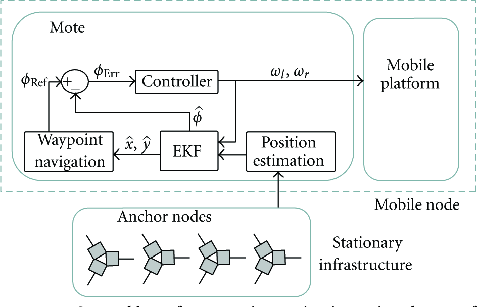
Figure 5 is a diagram of the control loop, which illustrates how the waypoint navigation system works. A mobile sensor node traverses the sensing region by moving from one waypoint to another. The waypoint coordinates are stored in the mote's memory. The mobile node observes the phase of interference signals transmitted sequentially by anchor nodes at known positions within the sensing region. Anchor bearings are estimated, from which the position of the mobile node, $(\widehat{x},\widehat{y})$ , is calculated using triangulation. These coordinates are then used by the waypoint navigation logic to determine if the mobile node has reached the next waypoint. If this is the case, a new heading ${\varphi }_{\text{Ref}}$ is computed and a course correction is determined based on the difference between the current estimated heading (obtained by the onboard digital compass) and the new computed heading. This heading offset, ${\varphi }_{\text{Err}}$ , is input into a simple controller, which appropriately updates the angular velocities of the wheels, ${\omega }_l$ and ${\omega }_r$ , in order to keep the mobile node on the correct trajectory to intercept the waypoint. This process runs continuously until the last waypoint is reached. We describe each step of this process in detail as follows.

Figure 5

Control loop for waypoint navigation.

4.1. Mobile Platform Kinematics

We use the following equations to describe the kinematic model of our two-wheel mobile platform with differential steering:

$$\begin{array}{cc}& \dot{x}=\frac{r\left({\omega }_r+{\omega }_l\right)}{\mathrm{2}}\cos \varphi ,\\ \dot{y}=\frac{r\left({\omega }_r+{\omega }_l\right)}{\mathrm{2}}\sin \varphi ,\\ \dot{\varphi }=\frac{r\left({\omega }_r-{\omega }_l\right)}{\mathrm{2}b},\end{array}$$

(5)

where x and y constitute the mobile node's position, ϕ is the heading, r is the wheel radius, b is the distance between the hub center of the driving wheel and mobile platform axis of symmetry, and ${\omega }_r$ and ${\omega }_l$ are the right and left wheel angular velocities, respectively. The speed of the mobile node is the magnitude of the velocity, and in terms of wheel angular velocity is represented as $|v|=r({\omega }_r+{\omega }_l)/\mathrm{2}$ .

4.2. Position and Heading Estimation

In order for a mobile node to travel between arbitrary waypoints, it is necessary to know its current position and heading. Having approximated the bearing of the mobile node from a sufficient number of anchors, we can estimate its position using triangulation. Triangulation is the process of determining the position of an object by using the bearings from known reference positions. When two reference points are used (Figure 6(a)), the target position will be identified as the third point in a triangle of two known angles (the bearings from each reference point) and the length of one side (the distance between reference points).

Figure 6

Triangulation. (a) As few as two bearings from known positions are required to estimate the position of a target. (b) Degenerate case where a third bearing is needed to disambiguate position. (c) Three bearings may not intersect at the same position.

The intersection of bearings can be calculated using the following equations:

$$\begin{array}{cc}& x=x_{\mathrm{2}}+\cos \left({\alpha }_{\mathrm{2}}\right)\frac{y_{\mathrm{2}}-y_{\mathrm{1}}-\tan \left({\alpha }_{\mathrm{1}}\right)\left(x_{\mathrm{2}}-x_{\mathrm{1}}\right)}{\cos \left({\alpha }_{\mathrm{2}}\right)\tan \left({\alpha }_{\mathrm{1}}\right)-\sin \left({\alpha }_{\mathrm{2}}\right)},\\ y=y_{\mathrm{2}}+\sin \left({\alpha }_{\mathrm{2}}\right)\frac{y_{\mathrm{2}}-y_{\mathrm{1}}-\tan \left({\alpha }_{\mathrm{1}}\right)\left(x_{\mathrm{2}}-x_{\mathrm{1}}\right)}{\cos \left({\alpha }_{\mathrm{2}}\right)\tan \left({\alpha }_{\mathrm{1}}\right)-\sin \left({\alpha }_{\mathrm{2}}\right)},\end{array}$$

(6)

where $(x,y)$ are the coordinates of the intersecting bearings (i.e., the position estimate of the mobile node), $(x_i,y_i)$ are the coordinates of the reference position (i.e., the anchor), and ${\alpha }_i$ is the bearing of the mobile node relative to the anchor.

When the position of the mobile node is directly between the two reference points (Figure 6(b)), two bearings are not sufficient to determine position because the mobile node could be located at any point on that axis. Therefore, a third bearing is required to disambiguate. However, three bearings may not intersect at the same point if any bearing is inaccurate (Figure 6(c)). Triangulation techniques are presented in [27–30], in which position estimation using more than two bearings is considered. The method we use is a least squares orthogonal error vector solution based on [10, 31], which is rapid, has low complexity, and still provides accurate position estimates from noisy bearing measurements.

Least squares triangulation using orthogonal error vectors works as follows. Figure 7 illustrates a simplified setup with a single anchor ( $T_i$ ) and mobile node (M). The actual bearing from the anchor to the mobile node is denoted by ${\beta }_i$ and the estimate by ${\widehat{\beta }}_i$ . Similarly, the vector pointing from the anchor position to the actual mobile node position is denoted by ${\mathbf{v}}_i$ and the vector pointing to the estimated mobile node position by ${\widehat{\mathbf{v}}}_i$ . Finally, we denote the difference between the actual and estimated bearing vectors as the orthogonal error vector ${\mathbf{e}}_i$ such that ${{\mathbf{e}}_i}^{⊺}{\widehat{\mathbf{v}}}_i=\mathrm{0}$ .

Figure 7

Least squares triangulation using orthogonal error vectors.

If we let ${\mathbf{a}}_i=\left[\begin{array}{c}\sin \hspace{0.17em}\hspace{0.17em}{\widehat{\beta }}_i\\ -\cos \hspace{0.17em}\hspace{0.17em}{\widehat{\beta }}_i\end{array}\right]$ , then the orthogonal error vector is formally defined as

$$\begin{array}{cc}& {\mathbf{e}}_i=\Vert \mathbf{M}-{\mathbf{T}}_i\Vert \sin \left({\widehat{\beta }}_i-{\beta }_i\right){\mathbf{a}}_i,\end{array}$$

(7)

where $\parallel \mathbf{M}-{\mathbf{T}}_i\parallel$ is the distance between the mobile node and anchor position vectors, ${\widehat{\beta }}_i-{\beta }_i$ is the Gaussian bearing noise with zero mean and variance ${\sigma }_i^{\mathrm{2}}$ , and ${\mathbf{a}}_i$ is the unit vector orthogonal to ${\widehat{\mathbf{v}}}_i$ .

The position of the mobile node can be represented as $\mathbf{M}={\mathbf{T}}_i+{\widehat{\mathbf{v}}}_i+{\mathbf{e}}_i$ . To remove ${\widehat{\mathbf{v}}}_i$ , we multiply by the transpose of ${\mathbf{a}}_i$ , resulting in

$$\begin{array}{cc}& {{\mathbf{a}}_i}^{⊺}\mathbf{M}={{\mathbf{a}}_i}^{⊺}{\mathbf{T}}_i+{\eta }_i,\end{array}$$

(8)

where ${\eta }_i=\parallel \mathbf{M}-{\mathbf{T}}_i\parallel \sin \hspace{0.17em}\hspace{0.17em}({\widehat{\beta }}_i-{\beta }_i)$ . Considering all anchors ( $i=\mathrm{1},\dots ,N$ ), we have a system of equations that takes the form:

$$\begin{array}{cc}& \mathbf{A}\mathbf{M}=\mathbf{b}+\eta ,\end{array}$$

(9)

where $\mathbf{A}=[{{\mathbf{a}}_{\mathrm{1}}}^{⊺},{{\mathbf{a}}_{\mathrm{2}}}^{⊺},\dots ,{{\mathbf{a}}_N}^{⊺}{]}^{⊺}$ and $\mathbf{b}=[{{\mathbf{a}}_{\mathrm{1}}}^{⊺}{\mathbf{T}}_{\mathrm{1}},{{\mathbf{a}}_{\mathrm{2}}}^{⊺}{\mathbf{T}}_{\mathrm{2}},\dots ,{{\mathbf{a}}_N}^{⊺}{\mathbf{T}}_N{]}^{⊺}$ . A least squares solution for estimating M is given by

$$\begin{array}{cc}& \widehat{\mathbf{M}}={\left({\mathbf{A}}^{⊺}\mathbf{A}\right)}^{-\mathrm{1}}{\mathbf{A}}^{⊺}\mathbf{b},\end{array}$$

(10)

where $\widehat{\mathbf{M}}$ is the position estimate returned by the triangulation using noisy bearing measurements from N anchors.

Using this method, a node can determine its position with as little as two anchors, the minimum required for triangulation. The localization algorithm outputs the estimated position of the mobile nodes: $\widehat{x}$ and $\widehat{y}$ ; however, it is unable to estimate orientation. Therefore, to obtain the heading estimate $\widehat{\varphi }$ , we use a digital compass attached to the mobile platform. An alternative software-based method to estimate heading without a digital compass is presented in Section 5.4.

4.3. Waypoint Navigation

The mobile node needs to follow a trajectory (reference heading) that will lead it to the next waypoint. The bearing from the node's current position to the waypoint is one such trajectory. However, when the mobile node is close to the waypoint, a small localization error can contribute to large reference heading error. Instead, we define the reference heading as the bearing from the previous waypoint (or the initial position estimate of the mobile node) to the next waypoint:

$$\begin{array}{cc}& {\varphi }_{\text{Ref}}=\{\begin{array}{cc}{\tan }^{-\mathrm{1}}\left(\frac{w_{y_i}-\widehat{y}}{w_{x_i}-\widehat{x}}\right)\hfill & \text{if}\hspace{0.17em}\hspace{0.17em}i=\mathrm{1}\hfill \\ {\tan }^{-\mathrm{1}}\left(\frac{w_{y_i}-w_{y_{i-\mathrm{1}}}}{w_{x_i}-w_{x_{i-\mathrm{1}}}}\right)\hfill & \text{if}\hspace{0.17em}\hspace{0.17em}i>\mathrm{1},\hfill \end{array}\end{array}$$

(11)

where $w_{x_i}$ and $w_{y_i}$ are the coordinates of waypoint i and $\widehat{x}$ and $\widehat{y}$ are the estimated position of the mobile node. Initially, ${\varphi }_{\text{Ref}}$ is computed based on the position of the mobile node and the first waypoint. After the mobile node has reached the first waypoint, ${\varphi }_{\text{Ref}}$ is calculated once for each waypoint i at the time waypoint $i-\mathrm{1}$ is reached.

Heading error is then determined by subtracting the mobile node's heading estimate, $\widehat{\varphi }$ , from the reference heading, ${\varphi }_{\text{Ref}}$ :

$$\begin{array}{cc}& \begin{array}{c}{\varphi }_{\text{Err}}={\varphi }_{\text{Ref}}-\widehat{\varphi }.\end{array}\end{array}$$

(12)

4.4. Mobile Sensor Control

To arrive at the wheel angular velocities that will keep the mobile sensor on the reference trajectory, we use a PI controller that takes the heading error ${\varphi }_{\text{Err}}$ as an input. Because the heading wraps to $\mathrm{0}$ at $\mathrm{2}\pi$ , we shift the heading error to fall between $-\pi$ and π:

$$\begin{array}{cc}& {\varphi }_{\text{Err}}=\{\begin{array}{cc}{\varphi }_{\text{Err}}-\mathrm{2}\pi \hfill & \text{if}\hspace{0.17em}\hspace{0.17em}{\varphi }_{\text{Err}}>\pi \hfill \\ {\varphi }_{\text{Err}}+\mathrm{2}\pi \hfill & \text{if}\hspace{0.17em}\hspace{0.17em}{\varphi }_{\text{Err}}<-\pi \hfill \\ {\varphi }_{\text{Err}}\hfill & \text{otherwise}.\hfill \end{array}\end{array}$$

(13)

The controller then takes the following form:

$$\begin{array}{cc}& \dot{\varphi }=K_p{\varphi }_{\text{Err}}\left(T\right)+K_i{T}_e\sum _{t=\mathrm{1}}^T‍{\varphi }_{\text{Err}}\left(t\right),\end{array}$$

(14)

where $K_p$ and $K_i$ are constant proportional and integral gains, respectively, T is the current sample number, ${\varphi }_{\text{Err}}(t)$ is the heading error for sample t, and $T_e$ is the time elapsed from the previous sample. The output of the controller, $\dot{\varphi }$ , is the updated angular velocity of the mobile node; however, the mobile platform is commanded by specifying an angular velocity for each wheel. Consequently, we convert $\dot{\varphi }$ into individual wheel angular velocities, ${\omega }_l$ and ${\omega }_r$ , as follows:

$$\begin{array}{cc}& {\omega }_l=\frac{\left|v\right|-b\dot{\varphi }}{r},\\ {\omega }_r=\frac{\left|v\right|+b\dot{\varphi }}{r}.\end{array}$$

(15)

Here, r and b (defined in Section 4.1) are system parameters with known values. $|v|$ is an input parameter to this system and does not change even though the mobile platform may not actually achieve the desired value. This is because we are only interested in regulating the heading, and not the speed, of the mobile platform.

The effect of the above transformation is that both wheels will be set with an equal desired base speed. If heading error exists, the controller will minimize it by turning one wheel faster than the base speed, and the other wheel slower, which will result in the mobile node turning in the correct direction as it moves forward. This type of controller has low runtime complexity and does not require a substantial amount of memory.

5. Error Analysis

In this section, we analyze the main sources of error in TripNav. We do this by generating a simulated setup and observing how various error sources affect the results. We also analyze the system assuming that a digital compass is not available. The simulation engine models the dynamics of the mobile node and computes the ideal bearings from each anchor at each timestep. Triangulation is then performed using the computed bearings. For the error analysis, Gaussian noise is added to the heading and position estimates, as described below for each source of error. In the simulation, we position anchors at the corners of a $20\times 20$ meter region. The mobile node follows a path that takes around a $10\times 10$ meter square within the sensing region. The desired speed of the mobile node is fixed first at 100 mm/s and then at 400 mm/s. This setup is identical to our real-world experimental evaluation, described in detail in Section 7 and illustrated in Figure 18.

5.1. Position Estimation Error

Although position error can reach as high as several meters in the worst case, it contributes relatively little to TripNav error. This is because position estimates are only used to recognize waypoint proximity. The rest of the time, the digital compass is used to maintain the desired trajectory. To analyze the effect of localization accuracy on TripNav, we simulate the system under ideal conditions, while adding Gaussian noise to the position with zero mean and varying the standard deviation between zero and five meters. Figure 8 shows the simulated paths of the mobile node with different localization accuracies. We see from the figure that even with large position error, the mobile node will still complete the circuit; however, the path it follows can be offset significantly from the desired path. Note that there are a greater number of data points for the 100 mm/s simulation because the mobile sensor is moving slower and can therefore perform more measurements.

Figure 8

TripNav trajectories due to position error when the mobile node speed is (a) 100 mm/s and (b) 400 mm/s.

5.2. Digital Compass Measurement Noise

In order to compute the heading error of the mobile node, its current orientation must be known. To determine this, we use a digital compass. To understand how noisy compass sensor data affects navigation, we performed 100 simulated runs under ideal conditions, introducing a Gaussian noise to the compass heading with zero mean and a standard deviation of 0.5°, 1°, 2°, 3°, 4°, and 5°. Figure 9 shows the average associated position error for each. From the figure, we see that even a compass heading error as high as 5° does not contribute significantly to the position error.

Figure 9

TripNav average position error due to digital compass sensor noise when the mobile node speed is (a) 100 mm/s and (b) 400 mm/s.

5.3. Latency

Because the mobile node is in motion while performing localization, the accuracy of the position estimate will depend on the speed of the mobile node and the latency of the localization algorithm. Bearings from each anchor are estimated sequentially. Triangulation is then performed to determine position by finding the intersection of these bearing vectors. However, even if all other sources of error were absent from this system, these bearing vectors would still not intersect at a common point because each measurement is made from a slightly different physical location. In addition, once all measurements have been taken, the mobile node continues to change its location while phase data is being transmitted from the anchor nodes and the position estimate is computed. Therefore, the faster the TripNav control loop runs, the more accurate the position estimates will be because the mobile node will not have had a chance to move far from the position where the localization algorithm was initiated.

To analyze how this affects the accuracy of TripNav, we simulate the system under ideal conditions while varying the number of anchors. We performed 100 simulated runs and averaged the position error for each localization. Figure 10 shows the average position error we can expect due to latency when we use two, three, and four anchors. From the figure, we can see that the latency incurred by increasing the number of anchors affects TripNav position accuracy on the order of centimeters.

Figure 10

TripNav average position error due to latency using 2, 3, and 4 anchors, when the mobile sensor speed is (a) 100 mm/s and (b) 400 mm/s.

5.4. Waypoint Navigation without the Digital Compass

The digital compass used in our implementation (see Section 6) is the Honeywell HMR3300 [32]. The compass has a compact footprint measuring 2.54 cm by 3.81 cm, is accurate up to 1° with 0.1° resolution and 0.5° repeatability, and has tilt compensation. However, the compass is expensive relative to the mobile sensor, and is therefore not an ideal solution.

Instead, it is possible to obtain our heading without the digital compass by computing the angle with respect to an arbitrary axis between the previous and current positions, as illustrated in Figure 11(a). The accuracy of the heading estimate will depend on the accuracy of the position estimates and assume that the mobile device takes the shortest path between the two positions. If in fact the mobile device does not move between the two positions along a straight line (see Figure 11(b)), the heading estimate could be highly inaccurate. This can be caused, for example, by uneven terrain, drive motor wear and tear, and wheel slippage. However, successive position measurements taken relatively close in time will minimize the amount of heading inaccuracy that can occur. An extended Kalman filter (EKF) can further improve the heading estimate, thereby eliminating the need for the digital compass.

Figure 11

(a) Computing the heading of the mobile device. (b) Heading inaccuracy will result if the mobile device does not travel in a straight line.

The EKF linearizes the estimation about the current state of the mobile node by applying the partial derivatives of the process and measurement functions, which take the form:

$$\begin{array}{cc}& X_k=F\left(X_{k-\mathrm{1}},u_k,w_{k-\mathrm{1}}\right),\\ z_k=h\left(X_k,v_k\right),\end{array}$$

(16)

where $X_k$ is the state of the mobile node $\{x,y,\varphi ,\dot{x},\dot{y}\}$ , $u_k$ is the process input $\{{\omega }_l,{\omega }_r\}$ obtained from the controller, $w_k$ is the process noise with covariance Q, $z_k$ is the set of position estimates obtained from the anchor nodes, $v_k$ is the measurement noise with covariance R, and k is the timestep. The heading estimate $\widehat{\varphi }$ is computed as the angle of the velocity vector $\{\dot{x},\dot{y}\}$ with respect to the x axis. Replacing the digital compass with the EKF in our waypoint navigation system results in the control loop pictured in Figure 12.

Figure 12

Control loop for waypoint navigation using the EKF for heading estimation.

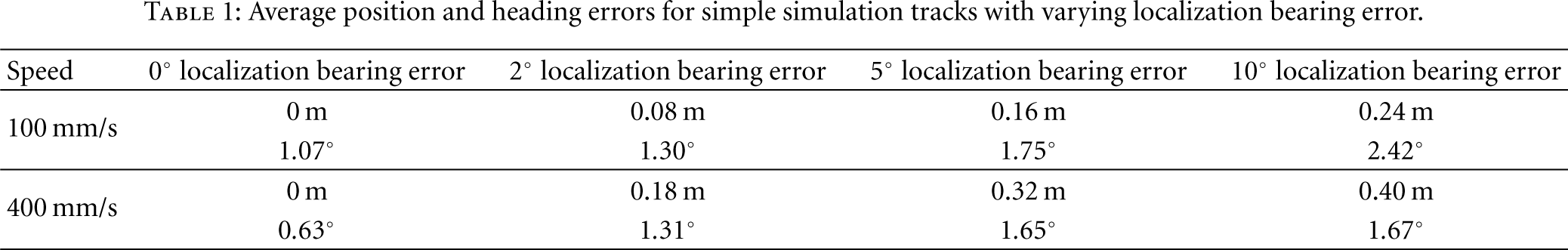
We ran simulations similar to our real-world experiments (see Section 7), both at 100 mm/s and 400 mm/s. For each set of simulations, we varied the bearing error of the localization algorithm (0, 2, 5, and 10 degrees). The wheel angular velocity error was fixed at 1 degree. The average position and heading errors for each simulation are listed in Table 1, and the tracks are pictured in Figures 13 and 14.

Table 1

Average position and heading errors for simple simulation tracks with varying localization bearing error.

Speed	${\mathrm{0}}^{\circ }$ localization bearing error	${\mathrm{2}}^{\circ }$ localization bearing error	${\mathrm{5}}^{\circ }$ localization bearing error	$\mathrm{1}{\mathrm{0}}^{\circ }$ localization bearing error
100 mm/s	0 m	0.08 m	0.16 m	0.24 m
	$\mathrm{1.0}{\mathrm{7}}^{\circ }$	$\mathrm{1.3}{\mathrm{0}}^{\circ }$	$\mathrm{1.7}{\mathrm{5}}^{\circ }$	$\mathrm{2.4}{\mathrm{2}}^{\circ }$
400 mm/s	0 m	0.18 m	0.32 m	0.40 m
	$\mathrm{0.6}{\mathrm{3}}^{\circ }$	$\mathrm{1.3}{\mathrm{1}}^{\circ }$	$\mathrm{1.6}{\mathrm{5}}^{\circ }$	$\mathrm{1.6}{\mathrm{7}}^{\circ }$

Figure 13

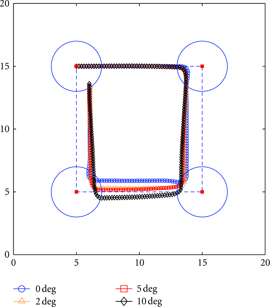
Simulations of mobile sensor waypoint navigation over a simple track at 100 mm/s using an EKF for heading estimation. Each track was run with different bearing errors of the localization algorithm.

Figure 14

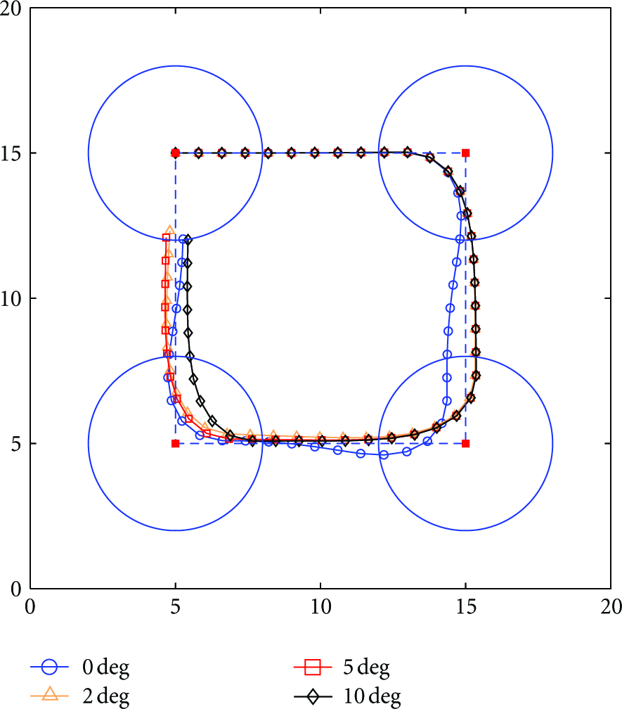
Simulations of mobile sensor waypoint navigation over a simple track at 400 mm/s using an EKF for heading estimation. Each track was run with different bearing errors of the localization algorithm.

In addition, we performed simulations over a more complex track similar to that used in [33]. The average position and heading errors for each simulation are listed in Table 2, and the tracks are pictured in Figures 15 and 16.

Table 2

Average position and heading errors for complex simulation tracks with varying localization bearing error.

Speed	${\mathrm{0}}^{\circ }$ localization bearing error	${\mathrm{2}}^{\circ }$ localization bearing error	${\mathrm{5}}^{\circ }$ localization bearing error	$\mathrm{1}{\mathrm{0}}^{\circ }$ localization bearing error
100 mm/s	0 m	0.23 m	0.47 m	0.86 m
	$\mathrm{0.4}{\mathrm{4}}^{\circ }$	$\mathrm{2.3}{\mathrm{7}}^{\circ }$	$\mathrm{3.0}{\mathrm{1}}^{\circ }$	$\mathrm{3.5}{\mathrm{0}}^{\circ }$
400 mm/s	0 m	0.26 m	0.52 m	0.87 m
	$\mathrm{1.3}{\mathrm{3}}^{\circ }$	$\mathrm{1.3}{\mathrm{6}}^{\circ }$	$\mathrm{1.6}{\mathrm{6}}^{\circ }$	$\mathrm{1.7}{\mathrm{1}}^{\circ }$

Figure 15

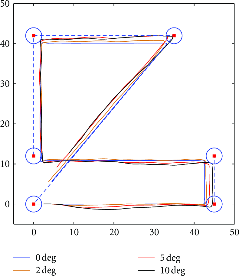
Simulations of mobile sensor waypoint navigation over a complex track at 100 mm/s using an EKF for heading estimation. Each track was run with different bearing errors of the localization algorithm.

Figure 16

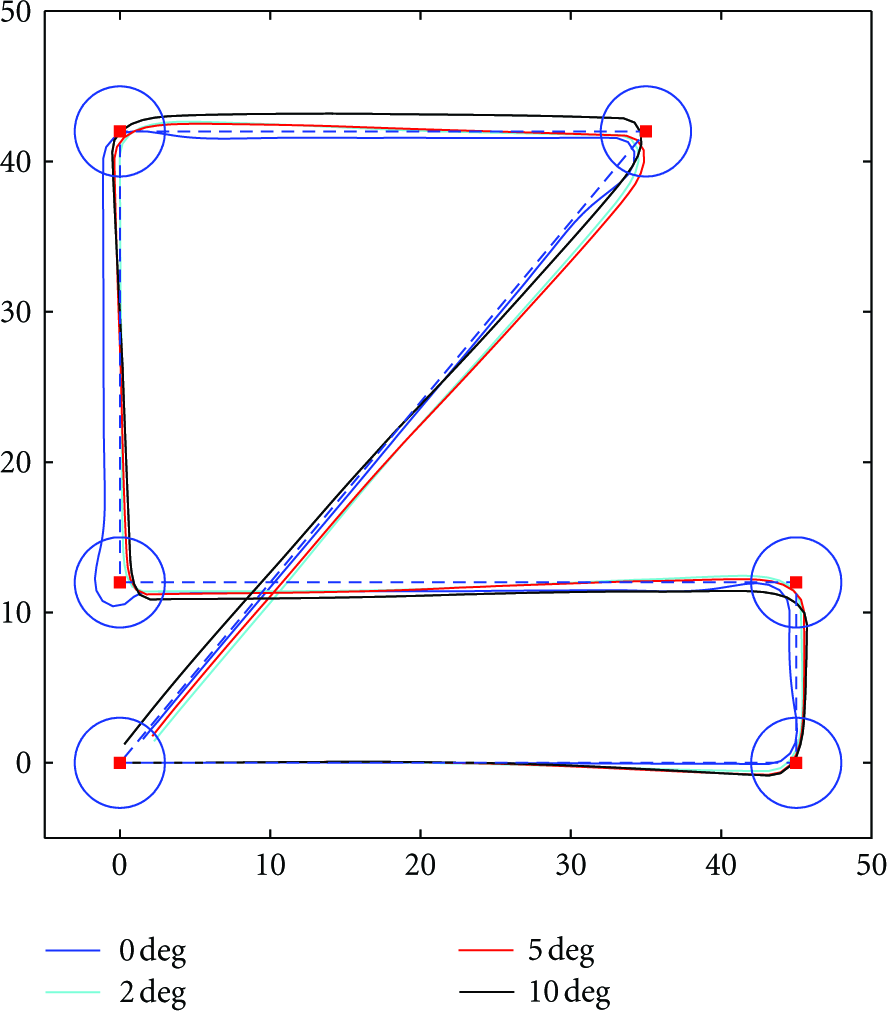
Simulations of mobile sensor waypoint navigation over a complex track at 400 mm/s using an EKF for heading estimation. Each track was run with different bearing errors of the localization algorithm.

It is clear from these simulation results that mobile sensor waypoint navigation can be achieved using the TripNav system without the need for a digital compass. This is beneficial to the overall system because we can still accurately maintain our desired trajectory without adding the weight, cost, and energy demand of additional hardware to the mobile platform.

6. Implementation

Our mobile sensor is comprised of an XSM mote [12] attached to an iRobot Create mobile platform [13], as pictured in Figure 17. All localization and control operations are performed on the mote, which communicates with the Create microcontroller over a serial interface. Mobile sensor heading is determined using a Honeywell HMR3300 digital compass [32]. The Create acts solely as a mobile platform and does not perform any computation or control independently of the mote. The anchor node implementation is described in [9].

Figure 17

The TripNav mobile platform.

Figure 18

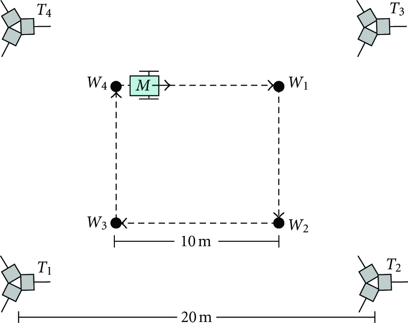
Waypoint navigation experimental setup. Anchors ( $T_{\mathrm{1}}\cdots T_{\mathrm{4}}$ ) surround the sensing region. The mobile node (M) is instructed to drive in a square, passing through each waypoint ( $W_{\mathrm{1}}\cdots W_{\mathrm{4}}$ ) before proceeding to the next.

The Create is a small-profile mobile platform, only 7.65 cm tall. Fixing the XSM mote to the Create body becomes problematic because the localization transmission signal is affected by ground-based reflections. We built a mount out of lightweight PVC pipe that places the mote 85 cm off the ground. We determined experimentally that 85 cm was sufficient to minimize the effect of ground-based reflections. The mount is fixed to the Create body, and houses the XSM mote, the digital compass, the connecting cable assembly for communicating with the Create and a battery pack.

One of the main implementation challenges for TripNav is designing an accurate rapid localization system as well as waypoint navigation and mobile control logic that is small enough to fit in the memory of a single mote. Our TripNav implementation consumes approximately 3.1 kB RAM and 60 kB of programming memory.

7. Experimental Evaluation

We place four anchors at the corners of a $20\times 20$ meter region in a nonmultipath outdoor environment. The mobile node is given as a series of four waypoint coordinates within the region and instructed to drive along the square route that connects the waypoints. Once the mobile node reaches the last waypoint (i.e., completes the circuit), it is instructed to come to a stop. Figure 18 illustrates this setup.

7.1. Performance Analysis

There are several tunable parameters for waypoint navigation using TripNav. Since TripNav only controls the heading of the mobile node and not its speed, an important system parameter is the target drive speed (the translational speed of the mobile node). The maximum speed of the Create is 500 mm/s. However, because we attached a sensor mount to the body of the Create, the increased weight (as well as uneven terrain) limits the speed to about 450 mm/s. Because the controller specifies wheel speeds such that one wheel may rotate faster than the target speed and the other slower, we set our maximum target drive speed to be 400 mm/s. For our experiments, we performed waypoint navigation with target drive speeds of 100 mm/s and 400 mm/s.

Because of localization error and continuous movement, the mobile sensor will not always be able to land exactly on the waypoint. We, therefore, select a waypoint range that specifies how close the mobile sensor must be to a waypoint before being allowed to proceed to the next. The size of the waypoint range is adjusted based on the speed of the mobile node and the latency of the localization. If the mobile node's speed is slower, we can reduce the size of the waypoint range. If the mobile node's speed is faster, we must increase the size of the waypoint range, otherwise the mobile node will not realize that it reached the waypoint. Because we make the design decision to not slow down as the mobile node nears the waypoint, or stop at the waypoint, turn, then start forward motion again, we must resort to using the waypoint range. For our experiments, we ultimately chose waypoint ranges of two meters when moving at 100 mm/s and three meters when moving at 400 mm/s. We found that if we increased the waypoint range beyond these values, the mobile node still completed its circuit; however, the path it followed had a high average position error.

Finally, to filter out inaccurate position estimates, we use a simple validation gate that approximates the distance traveled since the last position estimate by multiplying the elapsed time by the average wheel speed. If the distance difference between the current and previous position estimates is greater than the estimated travel distance plus a position error constant (to account for positioning and drive error), then the current position estimate is discarded. We chose a value of 2.5 meters for the position error constant.

We performed five waypoint navigation runs for both target drive speeds using TripNav. Figure 19 shows the average path of the mobile node over all runs. Note that the mobile node's path does not intersect with the waypoints and seems to stop short of the final waypoint. This is due to the waypoint range setting, where the mobile node considers the waypoint reached if it comes within the specified range. On average, position and heading accuracy with respect to the desired trajectory was 0.95 m and 4.75° when traveling at 100 mm/s and 1.08 m and 5.05° when traveling at 400 mm/s.

Figure 19

Waypoint navigation average position results when mobile sensor speed is (a) 100 mm/s, and (b) 400 mm/s. The dotted line represents the desired path. Waypoints are marked $W_{\mathrm{1}}\cdots W_{\mathrm{4}}$ , and the the surrounding circles represent the waypoint range of (a) 2 m and (b) 3 m.

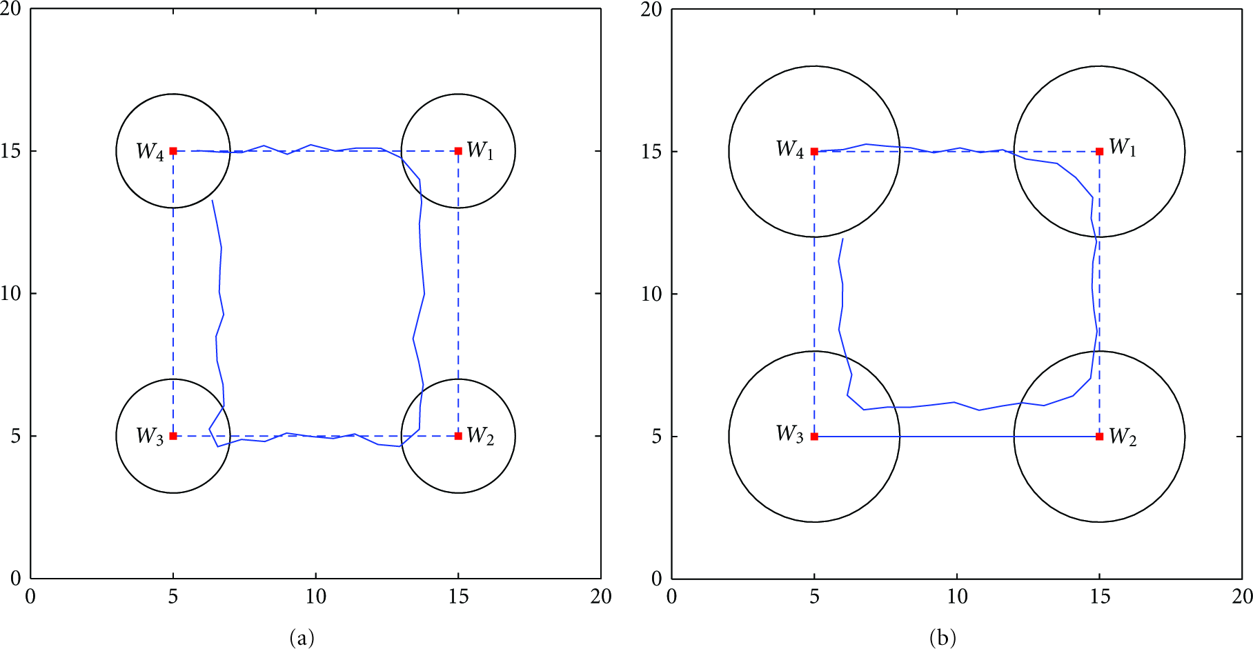
Figure 20 displays the outermost and innermost positions along the circuit of the mobile node over all runs. These are not individual paths, but bounds on the mobile sensor's movement over all five runs. This shows that one TripNav run does not significantly vary from another.

Figure 20

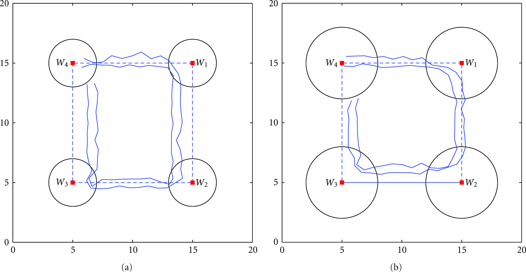
Waypoint navigation outermost and innermost path when mobile sensor speed is (a) 100 mm/s, and (b) 400 mm/s. The dotted line represents the desired path. Waypoints are marked $W_{\mathrm{1}}\cdots W_{\mathrm{4}}$ , and the the surrounding circles represent the waypoint range of (a) 2 m and (b) 3 m.

7.2. Latency Analysis

Since the mobile sensor is moving while estimating its position, localization must be performed rapidly, otherwise the mobile node will be in a significantly different location by the time a result is returned. The speed of the entire localization process depends on the latency of each component within the TripNav system, and so we provide a timing analysis of those components here. A latency analysis of the individual components involved in bearing estimation is presented in [9].

Figure 21 shows a sequence diagram for each step in the TripNav control loop, in which two anchors (dotted boxes) and a single mobile node are used. Because phase difference is used to determine bearing, each node must measure the signal phase at the same time instant. This requires synchronization with an accuracy on the order of microseconds or better. A SyncEvent message [26] is broadcast by the primary transmitter and contains a time in the future for all participating nodes to start the first RIM. Each array then performs two RIMs, one for each primary-assistant pair. Signal transmission involves acquiring and calibrating the radio, transmitting the signal, then restoring the radio to enable data communication. The assistant nodes in the array store their phase measurements until both primary-assistant pairs have finished their RIMs, at which point they broadcast their phase measurements to the mobile node. The mobile node calculates its bearing from each array, determines its position using triangulation, obtains its heading from the digital compass, and then uses this information to move in the appropriate direction.

Figure 21

Sequence diagram of the TripNav control loop in which two anchors are used.

Table 3 lists the average and maximum execution times over 100 iterations for the components pictured in Figure 5. Note that TripNav execution time depends on the number of participating anchors because bearing from each anchor is estimated sequentially. A minimum of two anchors is required for triangulation; however, the accuracy of the localization will improve with the addition of more participating anchors. We, therefore, provide execution times for three scenarios, in which we vary the number of participating anchors between two (the minimum required) and four (the number we use in our real-world evaluation).

Table 3

Latency of TripNav components.

Component	Average latency (ms)	Maximum latency (ms)
Digital compass	49.61	89.48
Waypoint navigation	0.45	0.52
Controller	0.64	0.68
Localization (2 anchors)	888.72	956.22
Localization (3 anchors)	1283.81	1334.99
Localization (4 anchors)	1667.76	1734.48

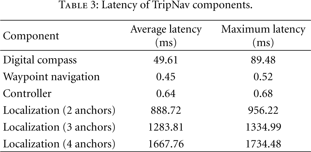
On average, the digital compass takes approximately 50 ms to estimate heading. This is in fact a limitation of the compass hardware, which provides heading estimates at a rate of approximately 8 Hz, or 125 ms. The 50 ms latency reflects the average time we must wait for the next heading estimate to be returned.

It is worth noting that because the mobile node acts solely as a receiver in this process, system latency is not affected by introducing more mobile nodes to the sensing region. TripNav is fully scalable in this respect; however, latency will increase as more anchors are employed, which will ultimately limit the size of the sensing region.

7.3. The Effect of TripNav Mobility on Position Accuracy

We performed our localization technique on a stationary sensor network deployment. Similar to the TripNav mobility experiments, four anchors were placed at the corners of a $20\times 20$ meter region in an outdoor environment. Twelve stationary target nodes, placed at least 2.5 m inside the sensing region, performed 50 position estimates each. The average localization error was 0.62 m.

The experiment demonstrates the effect of TripNav mobility on the accuracy of our localization technique. When the mobile node is moving at a speed of 100 mm/s, the average position error due to mobility is 0.33 m. At a speed of 400 mm/s, the average position error is 0.46 m.

8. Conclusion

Spatiotemporal awareness in mobile wireless sensor networks entails new challenges that result from integrating resource-constrained wireless sensors onto mobile platforms. The localization methods and algorithms that provide greater accuracy on larger-footprint mobile entities with fewer resource limitations are no longer applicable. Similarly, centralized and high-latency localization techniques for static WSNs are undesirable for the majority of MWSN applications. In this paper, we presented a waypoint navigation method for resource-constrained mobile wireless sensor nodes. The method is rapid, distributed, and has submeter accuracy.

One of the biggest challenges we face with RF propagation is multipath fading. Currently, TripNav will not work acceptably in multipath environments. Outdoor urban areas and building interiors are both major sources of multipath, and yet these are places where MWSNs have the greatest utility. An RF-based localization system that provides accurate results in these environments would be a major step forward. This is a future direction for our MWSN localization and navigation research, and we have already obtained encouraging preliminary results. In [34], we were able to demonstrate that precise RF indoor 1-dimensional tracking is indeed possible, and we are currently investigating how we can extend this technique to two and three dimensions. Such fine-grained RF-based localization would enable mobile sensors to navigate through hallways of burning buildings, help to evacuate shopping malls in the event of an emergency, and monitor the health of patients in every room of their house.