An Energy-Efficient Distributed Algorithm for Virtual Backbone Construction with Cellular Structure in WSN

Abstract

The construction of virtual backbone within wireless sensor network (WSN) is an important means to reduce the redundant transmission and conserve limited energy resources. However, if there is not a rotation scheme for the virtual backbone, the network lifetime is still considerably limited due to the quick exhaustion of the backbone Nodes' energy. In this paper, we propose an Energy-efficient Distributed algorithm for virtual backbone construction with Cellular structure (EDBC) in WSN. The algorithm combines optimal coverage theory based on cellular structure and energy consumption model for different kinds of sensor nodes to achieve the construction and rotation of backbone in multiple rounds. The simulation results have shown that it improves the balance of energy consumption among sensor nodes and extends the network lifetime. It also provides good network stability as the number of backbone nodes selected in each round remains small and relatively constant.

1. Introduction

The sensor nodes in wireless sensor network (WSN) are usually battery powered [1]. The energy resource of nodes is severely constrained and difficult to be recharged or replaced. It is necessary for the extension of network lifetime to decrease the unnecessary energy consumption by reducing the redundant transmission. The construction of virtual backbone is one of the important means to achieve these goals in wireless sensor networks [2, 3]. A smaller backbone will help to set up energy-efficient routing paths and conserve the energy of nonbackbone nodes which can switch into the energy-saving sleep mode when no monitoring tasks available. However, if there is not a rotation scheme for the backbone nodes, that is they continuously operate without being replaced by other nodes with more residual energy, the fast energy exhaustion of backbone nodes will become the bottleneck for the extension of network lifetime and lead to the unbalanced energy consumption among nodes.

Recently, there are many literatures that focus on the virtual backbone construction in wireless sensor networks [4–7]. One class of algorithms such as the typical EMISB [5] and OHCDS [6] algorithms utilizes the connected dominating set (CDS) in graph theory. In EMISB, the virtual backbone is constructed on the approximate minimum connected dominating set which is derived from the maximal independent set. With the rotation of backbone, the energy consumption is balanced among sensor nodes. As EMISB requires the two-hop neighbor knowledge, it incurs much message exchange and rapid energy dissipation of nodes. Meanwhile the redundancy in the number of backbone nodes increases as the scale and density of networks increase. In OHCDS algorithm, the CDS is derived from the minimal forwarding set based on the one-hop neighbor knowledge. However, the number of redundant backbone nodes of OHCDS is quite high especially in large-scale or high node density networks though it uses one-hop neighbor information. This adversely affects the network performance. Another class of algorithms uses geometric calculations to determine the locations of backbone nodes. The representative one is the Adaptive Broadcast Protocol (ABP) [7] which is founded on the theory that the hexagonal lattice is the most efficient arrangement of circles to cover the plane [8]. ABP applies the cellular structure (hexagonal lattice) to select the nodes which are nearest to the vertices of regular hexagons to be the backbone nodes. The vertices are also referred to as the strategic locations. Because the successive hexagons in ABP are created from the last backbone nodes as one vertex, the cellular structure is distorted and the strategic locations are not in the optimal positions once the nodes deviate from the locations of supposed vertices [9]. The distortion effect may propagate and get worse as approaching the boundary of the network. The distortion inevitably happens in real networks even with high node density and causes the algorithm failure.

In this paper, we propose an energy-efficient distributed algorithm for virtual backbone construction with cellular structure (EDBC). It uses a revised scheme to construct the virtual backbone. Unlike ABP, the cellular structure and each strategic location in EDBC are fixed without being changed by the actual location of nodes to minimize the distortion and enhance the reliability. Furthermore, the energy factors are introduced to fulfill the selection and rotation of backbone nodes in multiround to balance the energy consumption and prolong the network lifetime. The operation of EDBC is divided into rounds. Each round begins with the backbone setup phase, when the backbone nodes are selected, followed by the state-transition phase, when the nodes within the network perform data gathering and delivering functions. The simulation results show that EDBC algorithm achieves good reliability that the number of backbone nodes remains small and stable with different node densities, and the lifetime and energy efficiency of network are improved due to the balanced energy consumption.

The rest of this paper is organized as follows. Section 2 analyzes the problems and proposes the solutions. Section 3 describes the implementation of EDBC algorithm. Section 4 presents simulation results, and Section 5 concludes the paper.

2. Problem Statements

There are two important issues to be considered in EDBC algorithm. The first is the scheme of virtual backbone construction based not only on the cellular structure but on the energy level of nodes. The second is to determine the start or stop of a round to realize the multiround running.

2.1. The Construction of Virtual Backbone

The possible solution to combine the cellular structure with energy factors for the virtual backbone construction is using the distance to the strategic locations together with the energy level of nodes as the criteria to select backbone nodes. To eliminate the distortion effect, we use fixed cellular structure which means that all of the strategic locations are fixed. In the fixed cellular structure, the nearest nodes to the certain strategic locations with higher energy level will become the candidate for backbone nodes. The strategic location as the reference point for the backbone node to be selected is also termed as related strategic location to that backbone node.

As shown in Figure 1, suppose node A is the initiator of the algorithm which is also the first backbone node and its location is the first strategic location a. Node B which is A's farthest 1-hop neighbor with high energy level is chosen to be the second backbone node. Strategic location b can be calculated by use of similar triangle theory given by:

$$\begin{array}{c}\frac{l_{\text{AB}}}{R}=\frac{x_{\text{A}}-x_{\text{B}}}{x_{\text{A}}-x_b}=\frac{y_{\text{A}}-y_{\text{B}}}{y_{\text{A}}-y_b},\end{array}$$

(1)

where ( $x_{\text{A}},y_{\text{A}}$ ), ( $x_{\text{B}},y_{\text{B}}$ ), and ( $x_b,y_b$ ) are coordinates of backbone nodes A, B and strategic location b respectively, $l_{\text{AB}}$ is the distance between node A and B and R is the communication range of nodes.

Figure 1

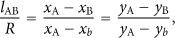
The backbone nodes selection in the fixed cellular structure.

Once the first edge $e_{ab}$ connecting strategic locations a and b are determined, the entire cellular structure and all the strategic locations are determined and fixed. For example, in Figure 1, the vertices a, b, c, and d form a geometric unit with three edges containing angles of 120 degrees. The coordinates of strategic locations c and d are calculated by the law of cosines as (2), given the coordinates of a and b:

$$\begin{array}{c}\frac{\mathrm{2}{R}^{\mathrm{2}}-\left[{\left(x_b-x_d\right)}^{\mathrm{2}}+{\left(y_b-y_d\right)}^{\mathrm{2}}\right]}{\mathrm{2}{R}^{\mathrm{2}}}=\cos \left(\frac{\mathrm{2}\pi }{\mathrm{3}}\right)=-\frac{\mathrm{1}}{\mathrm{2}},\\ {\left(x_a-x_d\right)}^{\mathrm{2}}+{\left(y_a-y_d\right)}^{\mathrm{2}}=R^{\mathrm{2}}.\end{array}$$

(2)

Among the 1-hop neighbors of backbone node A, the nodes such as nodes C and D, which are closest to their related strategic locations c and d, respectively and having higher energy level, become the candidate backbone nodes. This selection criterion is represented as the minimum of $R(i)$ as follows:

$$\begin{array}{c}R\left(i\right)=\alpha *\frac{E_{\text{ini}}-E\left(i\right)}{E_{\text{ini}}}+\frac{D\left(i\right)}{R},\end{array}$$

(3)

where for node i, $E_{\text{ini}}$ is its initial energy level, $E(i)$ is its energy level at the beginning of the current round, $D(i)$ is its distance to the related strategic locations, and parameter α is used to control the weight of energy factors in the decision on backbone nodes selection.

Similarly, we can calculate the coordinates of strategic locations e and f and select the candidate backbone nodes associated with e and f, respectively, from the set of 1-hop neighbors of node B. With the known coordinates of a, c, and d, another group of strategic locations g, h, I, and j are obtained, and subsequently the corresponding candidate backbone nodes are selected from 1-hop neighbor nodes of C and D, respectively. Repeating the process outward in the same way, all the strategic locations and associated candidate backbone nodes can be obtained.

2.2. Energy-Driven Multiround Operation

The rotation of backbone nodes in EDBC is implemented by multiround selection. The key to realize such operation is to determine the duration time of each round, which can be calculated based on the relationship between the energy consumption of nodes and time. This relationship can be derived by modeling the nodes' operation based on the theory of discrete-time Markov chain [10–12]. Because in each round, the energy consumption of nodes in setup phase is much lower than that of state-transition phase and thus can be ignored, only the energy consumption within state-transition phase is taken into account.

Within each discrete-time interval time_step, any node is in one definite state. If the node has S operation modes, its operation can be represented by the Markov chain with S states. According to the roles of nodes, there are three different types of nodes with different states in the network: the backbone nodes, nonbackbone nodes and isolated nodes.

When the virtual backbone is constructed, the clusters are organized. In state-transition phase, the backbone nodes act as cluster heads and mainly transfer data from nonbackbone nodes to the sink. Their 1-hop neighbor nodes, that is, the nonbackbone nodes, are the cluster members and perform the environmental monitoring and measuring tasks. The nodes beyond 1-hop radius from backbone nodes are isolated nodes and they do not participate in the data sensing and transferring tasks in current round. The modeling of these three types of nodes is presented as follows.

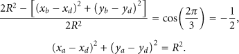
2.2.1. The State-Transition Model of Nonbackbone Node

Concerning one nonbackbone node in a cluster, the cluster head is backbone node i and the number of nonbackbone nodes as cluster members is $N_i$ . The nonbackbone node has four states: sending, receiving, idle, and sleep. The state diagram is shown in Figure 2, where p, q, and s are, respectively, the probability of transition from the idle state to the receiving state, from the idle state to the sending state and from the sleep state to the idle state. Because in the ordinary WSN, the nonbackbone nodes always send the data that they have sensed to the backbone nodes and seldom receive data or commands from the backbone nodes, thus $p\ll q$ and p is usually assigned a relatively small number (≈10⁻³). The sleeping time of the nonbackbone nodes is subject to the geometric distribution with parameter s[11, 12]. The probability q is

$$\begin{array}{c}q=g\times P_{\text{success}}.\end{array}$$

(4)

Figure 2

The state diagram of nonbackbone node.

For a nonbackbone node, g is the probability of generating one data packet during time_step and $P_{\text{success}}$ is the probability of its success in contending the channel with other nodes within the cluster. $P_{\text{success}}$ can be calculated by referring to CSMA/CA protocol specified by IEEE 802.15.4 [10] as:

$$\begin{array}{c}{P}_{\text{success}}=\iota \times {\left(\mathrm{1}-\iota \right)}^{{\stackrel{\sim }{N}}_i-\mathrm{1}}\times \left(\mathrm{1}-\gamma \right),\end{array}$$

(5)

where ι is the probability that clear channel assessment (CCA) is started in any slot and γ is the probability that the channel is occupied in one slot. ${\stackrel{\sim }{N}}_i$ is the number of nonbackbone nodes which are in idle state during one time_step. As $p,q\ll s$ , the probability $P_{\text{idle}}$ that the nonbackbone node is in idle state is $P_{\text{idle}}\approx (1-p-q)\times s\approx s$ and ${\stackrel{\sim }{N}}_i=N_i\times P_{\text{idle}}\approx N_i\mathrm{\hspace{0.17em}\hspace{0.17em}}\times s$ .

The average number of CCA executed by a node before it accomplishes data sending is given by

$$\begin{array}{lll}\bar{R}\hfill & =\hfill & (1-\gamma )+2\gamma (1-\gamma )+\cdots +(K-1){\gamma }^{K-2}(1-\gamma )\hfill \\ \hfill & \hfill & +K{\gamma }^{K-1}=\sum _{k=0}^{K-1}{\gamma }^k,\hfill \end{array}$$

(6)

where K is the number of backoff. The average time for sending one data packet is

$$\begin{array}{c}\stackrel{\_\_}{X}\mathrm{\hspace{0.17em}\hspace{0.17em}}=\mathrm{\hspace{0.17em}\hspace{0.17em}}{\sum }_{k=\mathrm{0}}^{K-\mathrm{1}}{\gamma }^k\left(b_k+\mathrm{1}\right)+\left(\mathrm{1}-{\gamma }^K\right)L,\end{array}$$

(7)

where $b_k$ is the average time of the $k_{\text{th}}$ backoff and L is the time required to send one data packet. Thus, γ and ι are represented as

$$\begin{array}{c}\iota =\frac{\stackrel{\_\_}{R}}{\stackrel{\_\_}{X}}=\frac{{\sum }_{k=\mathrm{0}}^{K-\mathrm{1}}{\gamma }^k}{{\sum }_{k=\mathrm{0}}^{K-\mathrm{1}}{\gamma }^k\left(b_k+\mathrm{1}\right)+\left(\mathrm{1}-{\gamma }^K\right)L},\\ \gamma =\frac{L\left(\mathrm{1}-{\left(\mathrm{1}-\iota \right)}^{{\stackrel{\sim }{N}}_i}\right)}{\mathrm{1}+L\left(\mathrm{1}-{\left(\mathrm{1}-\iota \right)}^{{\stackrel{\sim }{N}}_i}\right)}.\end{array}$$

(8)

Using (8), γ and ι can be calculated by iterative method. Thus, $P_{\text{success}}$ and then q can be obtained using (5) and (4) respectively.

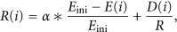
2.2.2. The State Transition Model of Backbone Node

The backbone node has three states: sending, receiving, and idle; it never goes into sleep state. The state diagram is shown as Figure 3. The probabilities of transition from the idle state to the sending or the receiving state are represented by α and β.

Figure 3

The state diagram of backbone node.

The probability of backbone node i receiving one packet during time_step includes two parts: the probability that one of its member nonbackbone nodes sends a packet is ${\stackrel{\sim }{N}}_i\times q_i\times (\mathrm{1}-q_i{)}^{{\stackrel{\sim }{N}}_i-\mathrm{1}}$ and the probability that one of its neighboring backbone nodes sends a packet. We assume that there are j neighboring backbone nodes of backbone node i and the probabilities of sending one packet for each of them are ${\alpha }_{i-\mathrm{1,1}},{\alpha }_{i-\mathrm{1,2}},\dots ,{\alpha }_{i-1,j}$ , respectively. Only one node can send packets in time_step, thus the probability that one neighboring backbone node sends a packet is

$$\begin{array}{c}{\sum }_{l=\mathrm{1}}^j\left({\alpha }_{i-\mathrm{1},l}\times \prod _{k=\mathrm{1},k\ne l}^j\left(\mathrm{1}-{\alpha }_{i-\mathrm{1},k}\right)\right).\end{array}$$

(9)

Because backbone node i mainly transfers the data that it has received and seldom sends packet to its member nonbackbone nodes, we can assume that ${\alpha }_i={\beta }_i$ and ${\beta }_i$ is consequently derived from the iteration process given as

$$\begin{array}{lll}{\beta }_i\hfill & =\hfill & {\stackrel{\sim }{N}}_i\times q_i\times {(1-q_i)}^{{\stackrel{\sim }{N}}_i-1}\times \prod _{k=1}^j(1-{\alpha }_{i-1,k})+{(1-q_i)}^{{\stackrel{\sim }{N}}_i}\hfill \\ \hfill & \hfill & \times \sum _{l=1}^j\left({\alpha }_{i-1,l}\times \prod _{k=1,k\ne l}^j(1-{\alpha }_{i-1,k})\right)(j\ne 0),\hfill \\ {\beta }_i\hfill & =\hfill & {\stackrel{\sim }{N}}_i\times q_i\times {(1-q_i)}^{{\stackrel{\sim }{N}}_i-1}(j=0)\hfill \end{array}$$

(10)

The probability α and β of each backbone node can be calculated using (10) starting from the leaf of the routing tree established by all the backbone nodes.

2.2.3. The State-Transition Model of Isolated Node

Though the isolated nodes do not participate in any operation of the network in the current round, they may become backbone nodes or nonbackbone nodes in next rounds. Hence the isolated nodes should always remain in one state—idle state, repeatedly listen to the channel until receive the initiation message launching new round and join the process of backbone nodes selection.

2.2.4. Duration Time of the Round

The duration of each round can be derived from the relationship between the energy consumption of nodes and time.

Suppose that the initial state of any node i is m. The number that the node is in state s during Ttime_steps is ${\sum }_{n=\mathrm{1}}^T{P}_{ms}(\mathrm{1},n)$ , where $P_{ms}(1,n)$ is the n-step transition probability. As the energy consumption of node i in state s within one time_step is $E_s=P_s\times time\_step$ , where $P_s$ is the power value for state s, its total energy consumption during T  time_steps is given as

$$\begin{array}{c}{E}_i\left(T\right)={\sum }_{s=\mathrm{1}}^S\left({\sum }_{n=\mathrm{1}}^T{P}_{ms}\left(\mathrm{1},n\right)\right)\times E_s.\end{array}$$

(11)

The state-transition model of backbone nodes and nonbackbone nodes can be proved to be time-homogenous Markov chains as p, q, α, and β are time-independent. It means that n-step transition matrix is the nth power of the single-step matrix. From Figures 2 and 3, the corresponding single-step transition matrix P and $P^{\prime }$ of nonbackbone node and of backbone node can be obtained, respectively,

$$\begin{array}{c}P=\mathrm{\hspace{0.17em}\hspace{0.17em}}\left[\begin{array}{cccc}\mathrm{0}& q& p& \mathrm{1}-q-p\\ \mathrm{1}& \mathrm{0}& \mathrm{0}& \mathrm{0}\\ \mathrm{1}& \mathrm{0}& \mathrm{0}& \mathrm{0}\\ s& \mathrm{0}& \mathrm{0}& \mathrm{1}-s\end{array}\right],\\ P^{\prime }=\left[\begin{array}{ccc}\mathrm{1}-\alpha -\beta & \alpha & \beta \\ \mathrm{1}& \mathrm{0}& \mathrm{0}\\ \mathrm{1}& \mathrm{0}& \mathrm{0}\end{array}\right].\end{array}$$

(12)

Thus using (12), the n-step transition probability $P_{ms}(1,n)=P_{ms}(n)$ for backbone nodes is the entries in the mth row and the sth column of transition matrix $P^{\prime n}$ and for nonbackbone nodes it is the entry of $P^n$ . With $P_{ms}(1,n)$ and (11), we can obtain the relationship between the energy consumption and time for all the backbone nodes and nonbackbone nodes within one round. The energy consumption of isolated nodes which always remain in idle state is linear with time.

For any node i, a threshold $E_{\lim }(i)$ is defined as

$$\begin{array}{c}{E}_{\lim }\left(i\right)=\min \left(b\times E\left(i\right),E\left(i\right)-E_{\text{th}}\right),\end{array}$$

(13)

where $E_{\text{th}}$ is the residual energy of a node that it can be regarded to be dead and constant parameter $0<b<1$ . If the energy consumption of any node meets the threshold, that is, $E_i(T)\ge E_{\lim }(i)$ , it can broadcast a initiation message to launch a new round. Given the threshold and relationships of energy consumption and time for all nodes, the duration time τ of the current round can be determined as the minimum value of T that satisfies

$$\begin{array}{c}\forall i\in \text{NODE},\hspace{0.17em}\forall T\in N^{+},\hspace{1em}\exists E_i\left(T\right)>E_{\lim }\left(i\right),\end{array}$$

(14)

where NODE denotes the set of all the nodes within the network.

3. Detailed Algorithm

3.1. Network Assumptions

We assume that the target region is a rectangular area and sensor nodes are randomly deployed in the region. The initiator of EDBC algorithm locates in the middle. All the nodes are location-aware and homogeneous in terms of initial energy, communication, and computing capabilities. The communication range is R and the initial energy level is $E_{\text{ini}}$ . All nodes learn their 1-hop neighbor information by neighbor discovery.

3.2. Setup Phase

EDBC algorithm runs in multiple rounds. In setup phase of each round, the backbone nodes are selected by applying the principle presented in Section 2.1.

Step 1.

Initialize the required parameters of EDBC, such as the number of nodes, the area of target region and the values of $E_{\text{ini}}$ , $E_{\text{th}}$ , time_step,g,s,p,α, and $\hspace{0.17em}\hspace{0.17em}L$ .

Step 2.

Determine the initial two backbone nodes and the related strategic locations. The initiator and the first backbone node A sets its location as the first strategic location a. It lists its one-hop neighbor nodes in a descending order according to (15) and then chooses the first one such as node B, which is farthest to A and has high energy level, to be the second backbone node:

$$\begin{array}{c}a*\frac{E\left(i\right)}{E_{\text{ini}}}+\frac{D\left(i\right)}{R}.\end{array}$$

(15)

Node A calculates the second strategic location b by using (1) and then informs backbone node B of the coordinates of a and b to be used by B to calculate the next strategic locations.

Given the strategic locations a and b, the cellular structure is fixed, go to Step 3 to compute the successive strategic locations and select the corresponding backbone nodes.

Step 3.

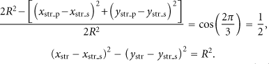
Calculate the successive strategic locations. Among the obtained backbone nodes, suppose BN stands for the current backbone node which will apply the law of cosines to calculate the next strategic location which is denoted by str_s. The related strategic location of BN and BN's last one-hop backbone node is represented by str and str_p, respectively. The coordinates of str_s can be calculated as follows:

$$\begin{array}{c}\frac{\mathrm{2}{R}^{\mathrm{2}}-\left[{\left(x_{\text{str}\_\text{p}}-x_{\text{str}\_\text{s}}\right)}^{\mathrm{2}}+{\left(y_{\text{str}\_\text{p}}-y_{\text{str}\_\text{s}}\right)}^{\mathrm{2}}\right]}{\mathrm{2}{R}^{\mathrm{2}}}=\cos \left(\frac{\mathrm{2}\pi }{\mathrm{3}}\right)=\frac{\mathrm{1}}{\mathrm{2}},\\ {\left(x_{\text{str}}-x_{\text{str}\_\text{s}}\right)}^{\mathrm{2}}-{\left(y_{\text{str}}-y_{\text{str}\_\text{s}}\right)}^{\mathrm{2}}=R^{\mathrm{2}}.\end{array}$$

(16)

Step 4.

Verify that the coordinates of str_s are in the reasonable range given by

$$\begin{array}{c}{x}_{\min }-adb<x_{\text{str}\_\text{s}}<x_{\max }+adb,\\ y_{\min }-adb<y_{\text{str}\_\text{s}}<y_{\max }+adb,\end{array}$$

(17)

where ( $x_{\max },y_{\max }$ ) and ( $x_{\min },y_{\min }$ ) define the target region.

If true, go to Step 5 to select candidate backbone node. Else, go to Step 3 to calculate other strategic locations.

Step 5.

Select the candidate backbone node related to strategic location str_s. BN lists its one-hop neighbor nodes in the order given by (18) and selects the smallest one to be the candidate backbone node. If the distance of the candidate to str_s is larger than a threshold th, the candidate is abandoned and go to Step 3. Otherwise BN informs the candidate of the coordinates of str and str_s:

$$\begin{array}{c}a\times \frac{E_{\text{ini}}-E\left(i\right)}{E_{\text{ini}}}+\frac{D\left(i\right)}{R}.\end{array}$$

(18)

Step 6.

Check for the existence of backbone nodes within one-hop radius from the candidate. If yes, the candidate becomes nonbackbone node. Else, the candidate becomes backbone node.

Step 7.

If no more backbone node is selected, setup phase ends. Otherwise, go to Step 3.

The expansion of region border by $adb$ in Step 4 intends to increase the number of backbone nodes in the border area because usually there are not enough nodes near the strategic locations especially near the border.

3.3. Station-Transition Phase

After setup phase is completed, station-transition phase starts and the normal functions of WSN are carried out. The duration of current round is determined to control the trigger of a new round.

Step 1.

Establish the state-transition models of all the backbone nodes, nonbackbone nodes and isolated nodes. By applying (11) with the transition matrixes P and $P^{\prime }$ , the quantitative relationship of every node between the energy consumption $E_i(T)$ and time T is obtained.

Step 2.

Determine the duration time τ of the current round by using (14).

Step 3.

Update the energy value of each node after time τ, that is, for all $i\in \text{NODE}$ , $E(i)\Leftarrow E(i)-E_i(\tau )$ and check whether the network is dead. If the residual energy level of any node satisfies (19), the network dies and EDBC algorithm stops. Else go to setup phase to start a new round:

$$\begin{array}{c}\forall i\in \text{NODE},\hspace{1em}\exists E\left(i\right)\mathrm{\hspace{0.17em}\hspace{0.17em}}<\mathrm{\hspace{0.17em}\hspace{0.17em}}{E}_{\text{th}}.\end{array}$$

(19)

3.4. Complexity of Algorithm

In the setup phase of EDBC algorithm, the complexity is introduced by two parts. (1) In the process to select the backbone nodes, each backbone node BN calculate the next strategic location str_s by using law of cosines and sorts its one-hop neighbors to select the candidate backbone node related to str_s. (2) The candidate checks the existence of backbone nodes among its one-hop neighbors before it can become the backbone node. Thus, the sorting and checking operations are conducting within the set of one-hop neighbor nodes. If we adopt Bubble Sort method, the complexity of the algorithm in the set-up phase is O(Δ), where Δ is the average degree of nodes in the network.

In the state-transition phase, the algorithm only involves the simple algebraic operations to calculate the corresponding state-transition probabilities and establish the transition model for every node. For the nonbackbone nodes, the calculations are performed on each node independently. For the backbone nodes, the calculations are carried out in a recursive process along the backbone. Thus, the complexity of state-transition phase is O( $N_{\text{BN}}$ ), where $N_{\text{BN}}$ indicates the number of backbone nodes which is considerably less than the number of nodes in the network.

4. Simulations

We present simulation experiments to test and compare the performance of EDBC with some other algorithms. One experiment verifies the stability in the size of backbone constructed by EDBC in comparison with EMISB, ABP, and OHCDS as the network density increases. Another experiment compares the effectiveness of backbone rotation for the balanced energy consumption of EDBC, EMISB, and a former version of EDBC without backbone rotation scheme—DBC [9].

4.1. Simulation Initialization

Simulations are carried out in 100 different topologies and the mean values are taken as the final results. Each topology is created as follows: nodes are randomly deployed in a $\mathrm{1800}\hspace{0.17em}\text{m}\times \mathrm{1800}\hspace{0.17em}\text{m}$ square region, the number of nodes varies from 300 to 1800 with the increment of 300, and the communication range R of each node is 240 m. The parameters in Markov model are initialized as follows: the initial energy of each node $E_{\text{ini}}=0.1\hspace{0.17em}J$ , $time\_step=4.8\hspace{0.17em}\text{ms}$ , $g=0.5$ , $s=0.12$ , $P=0.001$ , $L=5$ slots, and the values of average power in each state refer to the specification of the prototype node we have developed [13]. Other parameters are given as follows: $E_{\text{th}}=0.02\hspace{0.17em}J$ , $adb=R$ , $\text{th}=2R$ , the weight $\alpha =3$ or $\alpha =4$ , and constant $b=0.1$ .

4.2. Results and Analysis

4.2.1. Evaluation of the Stability in the Size of Virtual Backbone

As shown in Figure 4, the number of backbone nodes selected by EDBC and ABP remains stable despite the increase of network density. In comparison, the backbone size increases fast in EMISB when the number of nodes is more than 900. The backbone size in OHCDS increases almost linearly with the variation of network density because of its inherently high redundancy drawbacks. The result indicates that the cellular-structure-based algorithms including EDBC and ABP have good performance with small-sized virtual backbone to cover the 2D plane. EDBC algorithm surpasses ABP in decreasing the redundancy of backbone nodes by using a revised scheme with fixed cellular structure. The number of backbone nodes in EDBC is about 50% less than that in ABP algorithm. Meanwhile in the network with high density, the selected backbone nodes will be more nearer to the strategic locations and the real hexagons formed by the backbone nodes will be more close to the ideal ones. Thus, the number of backbone nodes is more stable in dense networks.

Figure 4

The size of backbone versus the number of nodes in the network.

4.2.2. Evaluation of the Network Lifetime and Efficiency of Energy Usage

The results to evaluate the effectiveness of backbone rotation scheme in EDBC, compared with EMISB and DBC in terms of network lifetime and efficiency of energy usage, are given in Figures 5 and 6. The network lifetime is defined as the time until the first node dies (FND). The efficiency of energy usage is the ratio of total energy consumption to the sum of initial energy for all nodes during network lifetime.

Figure 5

The network lifetime versus the number of nodes.

Figure 6

The efficiency of energy usage versus the number of nodes.

From the results between EDBC and DBC, it is obvious that the rotation of backbone contributes greatly to the improvement of energy usage efficiency and network lifetime. If there is not a backbone rotation scheme, like DBC algorithm, the network will die quickly when the energy of backbone nodes is depleted. In addition, due to the fact that there are many nonbackbone nodes still having much residual energy at the time of network death, the efficiency of energy usage is considerably low.

EDBC excels EMISB in the performance concerning the impact of network density. Both of them present the similar efficiency of energy usage and network lifetime in the scenarios with lower network density. However, in the case of higher density, the efficiency of energy usage and network lifetime of EMISB decrease while those of the EDBC still remain good. This is because that the rotation scheme of EMISB depends on much more multihop information and it leads to the redundancy of backbone nodes and high energy consumption of nodes for message exchange as the number of nodes increases.

Though the increase of the weight α in EDBC can improve the efficiency of energy usage and network lifetime, it also leads to more deviation of backbone nodes from the strategic locations of the fixed cellular structure. Thus, more isolated nodes will emerge and impairs the communication coverage of the region. There is upper bound for the improvement of energy efficiency by increasing the weight of energy factors. In our simulations, the network performance is best when $\alpha =4.0$ .

5. Conclusions

In this paper, we propose the algorithm EDBC to construct virtual backbone with a fixed cellular structure to minimize the distortion effect. It also establishes energy consumption model for all sensor nodes based on the theory of discrete-time Markov chain to control the rotation of backbone in multiple rounds. In each round, the backbone nodes will be replaced by new ones with higher energy level for balanced energy consumption. The simulation results show that EDBC constructs the backbone with smaller size and better stability than other algorithms, almost unaffected by the increase of node densities. Meanwhile the efficiency of energy usage is improved in EDBC and thus the network lifetime is prolonged.