A Distributed Algorithm for Virtual Backbone Construction with Cellular Structure in WSNs

Abstract

The normal node in wireless sensor networks (WSNs) often has no constant energy supply. To make efficient use of limited energy resources significant, a major way to save limited energy resources is constructing a smaller virtual backbone in WSNs. In this paper, we propose a distributed algorithm for virtual backbone construction with cellular structure in WSNs (DBC), which is an improvement of algorithm ABP (Duresi and Paruchuri, 2008) and minimize the distortion of constructed cellular structure by improving the way of calculating strategic points using 1-hop neighbor information. Our simulation results show that algorithm DBC has smaller virtual backbone than algorithm ABP, and the number of backbone nodes is much fewer than that one.

1. Introduction

The energy supply of nodes in wireless sensor networks (WSNs) is normally battery powered. As battery energy is limited and battery replacement or recharging is usually impractical for WSNs, it is significant to reduce energy consumption by redundancy transmission to prolong network working hours. Constructing virtual backbone is one of major ways to save limited network resources and optimize network performance [1, 2]. A smaller virtual backbone will not only benefit the design of energy-efficient routing, but also save energy of nondominated nodes which can enter sleep (energy-saving) mode without monitoring task.

At present, researchers [3–11] focus on virtual backbone construction in WSNs. There are two major methods.

The first method is constructing a virtual backbone by calculating the minimum connected dominating sets (MCDS). As calculating MCDS of arbitrary graphs is a NP-complete problem, heuristic algorithms are usually used. Algorithm MISB [3] and algorithm OHDC [4] are two typical distributed algorithms. Algorithm MISB constructs virtual backbone by calculating MCDS on the basis of maximum independent set. The number of backbone nodes calculated from algorithm MISB is fluctuant according to the node density or scale. As network size is increasing, the backbone nodes also increase their redundancy. Furthermore, algorithm MISB needs two hops neighbor information to calculate MCDS. As a result, more messages are exchanged, which means more energy consumption and more time delay. Algorithm OHDC also constructs virtual backbone by calculating MCDS. Comparing with algorithm MISB, algorithm OHDC uses only 1-hop neighbor information; however, the backbone nodes' redundancy is higher. Especially when the network size is large or the density of nodes is high, the redundancy will seriously affect the WSN performance.

The second method is constructing a virtual backbone by generating a hierarchy topology of entire network. Paruchuri et al. [5, 7, 8] proposed algorithms based on the theory that hexagonal lattice arrangement is the most efficient way for circles covering a plane surface. These algorithms use delay mechanism to select backbone nodes without any neighborhood knowledge. However, the cellular structure constructed during the process of selecting backbone nodes is distorted seriously which results in the situation that the algorithm can fail to deliver all the recipients connected to the source, even for highly connected networks. The representative of these algorithms is ABP [5].

In this paper, a distributed algorithm, named virtual backbone construction with cellular structure in WSNs (DBC), is proposed, which is an improved algorithm of algorithm ABP. The algorithm minimizes the distortion of constructed cellular structure and has better reliability and lesser backbone nodes by improving the method of selecting backbone nodes and the way of constructing cellular structure. Simulation results show that the number of virtual backbone nodes calculated by algorithm DBC is much fewer than those of original algorithms and almost constant for the same network areas with different node density. The results also show that DBC is fit for large scale WSNs.

The rest of this paper is organized as follows. Section 2 describes terms used in this paper. Section 3 analyses the problem and gives the solutions. Section 4 presents details of our algorithm. Section 5 presents performance evaluation. Section 6 concludes the paper.

2. Terms Description

Terms used in this paper are shown in Table 1. We assume that the transmission radius of each node is R, and all nodes are randomly deployed in a 2-dimensional geographical region.

Table 1

Terms table.

Initiator	The initial node with which algorithm DBC started
Backbone nodes (BN)	The nodes selected by algorithm DBC and made up the virtual backbone (including the initiator)
Candidates	The intermediate state of nodes. Before node becomes backbone node during the process of selecting backbone nodes
Strategy point (SP)	Vertices of hexagons in the cellular structure
Related node (RN)	In the one-to-one relationship between strategy points and backbone nodes, the backbone node is the related node of a strategy point
Related point (RP)	RP is the related strategy point of certain backbone node in the one-to-one relationship between strategy points and backbone nodes
Father strategy point (FSP)	During the DBC process, RP will be FSP of the next hop BN's RP
Son strategy point (SSP)	During the DBC process, the next hop BN's RP is the SSP of the last hop BN's RP

3. Problem Statement

Kershner [6] has proved that hexagonal lattice arrangement is the most efficient arrangement of circles covering the plane. There are two ways to construct the virtual backbone based on the hexagonal lattice (cellular structure), one is the distributed method, where locations of strategy points depend on locations of local selected backbone nodes; another is the centralized method, where location of each strategy point is fixed and cellular structure is determined.

3.1. Distributed Method

As shown in Figure 1, BN A is SP a's RN, and BN B is SP b's, besides BN A is BN B's last hop BN. With the line $\overline{BA}$ between BN A and BN B as reference edge of regular hexagons, calculate SP c and SP f, so that edge $\overline{Bf}$ and edge $\overline{Bc}$ both satisfy that its length is equal to the side of regular hexagon and it forms an 120 degree angle with reference edge $\overline{BA}$ . Then select node C which is closest to SP c as its RN. In the same way, SP d and SP e can be selected. And keep on executing these processes until strategy points and backbone nodes of the entire network are selected.

Figure 1

The distributed method of constructing virtual backbone.

Algorithm ABP adopts this distributed method. Source node s locates at the centre of certain regular hexagon. It starts the process of broadcasting messages for constructing virtual backbone. The message contains locations of the current sender and last sender (for source node s, the two locations are same). After nearby nodes received the message, they will calculate the distance to the strategic point from position information included in the message and then set a time delay which varies with the distance, so the node closest to certain strategy point should become backbone node and broadcast the message with locations of current sender and last sender. Algorithm ABP is a distributed algorithm; it is easier to achieve this distributed method by setting time delay. However, as Figure 1 shows obviously, the cellular structure constructed in this way is not uniformed as expected, as it is impossible that every strategy point has a node in realistic networks. What is more, the distortion is magnified gradually using distributed method, and the structure will get more twisted as closer to the boundary of the network. As a result, the communication coverage of the obtained virtual backbone is not unreliable, and there might be a lot of nodes which cannot connect any backbone node within 1-hop.

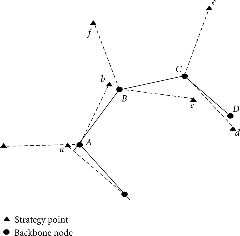
3.2. Centralized Method

Another is the centralized method, which means that locations of all strategy points are fixed and not affected by the positions of nodes, as long as any edge of certain regular hexagon is determinated. As shown in Figure 2, the initiator is node A whose position is the first strategy point a and chose its 1-hop neighbor node B which is farthest to node A as the second backbone node. Then utilizing similar triangle theory shown in Figure 3, calculate SP b by (1), in which $(x_A,y_A)$ is the location of BN A, and $(x_B,y_B)$ is BN B's, $(x_b,y_b)$ is SP b's, and $l_{AB}$ is the distance between BN A and BN B

$\frac{l_{AB}}{R}=\frac{x_A-x_B}{x_A-x_b}=\frac{y_A-y_B}{y_A-y_b}.$

(1)

Figure 2

The centralized method of constructing virtual backbone.

Figure 3

The schematic diagram of calculating SPs.

As the positions of SP a and SP b are determinated, according to the cellular structure, the locations of all the other strategy points in the network are fixed. As Figure 2 shows, vertices a, b, c, and d form a geometrical unit of which three edges form an 120 degree angle with each other, then calculate locations of all strategy points based on this geometrical unit. Utilizing cosine law shown in Figure 3, calculate SP c and SP d by (2) with known locations of SP a and SP b

$\begin{array}{c}\frac{2R^2-\left[{\left(x_b-x_d\right)}^2+{\left(y_b-y_d\right)}^2\right]}{2R^2}=\cos \left(\frac{2\pi }{3}\right)=-\frac{1}{2},\\ {\left(x_a-x_d\right)}^2+{\left(y_a-y_d\right)}^2=R^2.\end{array}$

(2)

Then select RN C for SP c and RN D for SP d in 1-hop neighbor nodes of BN A by (3), in which $D(i)$ means the distance between node i and certain SP and $N(A)$ means the set of BN A's all 1-hop neighbor nodes. Calculate locations of SP e and SP f and select RNs, respectively, from 1-hop neighbor nodes of BN B in the same way. And then locations of SPs g, h, i, and $\mathrm{\hspace{0.17em}\hspace{0.17em}}j$ can be obtained by locations of SPs a, c, and d, and their RNs will be chosen from 1-hop neighbor nodes of BN C and BN D. Execute this process along directions shown in Figure 2; locations and RNs of all RPs in the entire network are selected

$\mathrm{\hspace{0.17em}\hspace{0.17em}}{D\left(i\right)|}_{i=j}=\underset{i\in N\left(A\right)}{\min }\left(D\left(i\right)\right).$

(3)

Algorithm DBC adopts this centralized method, after initiator and second BN were determinate; locations of all the other SPs are determinated according to the cellular structure. What is more, each time we select a new BN, the distortion of constructed cellular structure will be amended as far as possible, so the communication coverage of obtained virtual backbone will be closest to the optimal coverage of ideal cellular structure, and the size of obtained virtual backbone is smaller than that of virtual backbone obtained from the distributed method. It is obvious that obtained virtual backbone will be closer to ideal case with higher node density, no matter through which method. That is why algorithm DBC has a better performance in the network with a higher node density.

4. Algorithm DBC

Assume that network area is a rectangle, and the initiator is at the center of the rectangle. Algorithm DBC comprises initiator subalgorithm described in Section 4.2 and backbone node subalgorithm described in Section 4.3.

4.1. Network Model and Assumptions

In this section, description about the network model and assumptions used in our algorithm DBC are provided.

• (1)

The initiator is at the center of the network area, and other nodes are randomly deployed in a two-dimensional geographical region.

(2)

Communication range: node is the center of a circle with radius R, and R is also the communication range.

(3)

All sensor nodes are homogeneous in terms of energy, communication, and processing capabilities.

(4)

All sensor nodes are location aware; that is, they are equipped with a GPS device.

(5)

All sensor nodes learn their 1-hop neighbor information including IDs and locations by neighbor discovery.

4.2. Initiator Subalgorithm

• (1)

  The initiator A sets its position as the first strategy point a, then chooses its 1-hop neighbor B which is the farthest to node A as a candidate, and then calculates SSP b (node B's RP) by (1). After that, initiator A sends candidate notice (CN) message containing locations of SP a and SP b to candidate B.

• (2)

  Calculate SSP c and SSP d by (2).

• (3)

  Select candidate C for SP c and candidate D for SP d within 1-hop neighbors of BN A by (3), which ensures the closest node to certain RP can be selected as far as possible. Then initiator A sends CN message containing locations of SP a and SP c or SP d to candidate C or candidate D.

• (4)

  End.

4.3. Backbone Node Subalgorithm

• (1)

  After received CN message, Candidate $b{n}_{pt}$ sends messages to $N(b{n}_{pt})$ to check out if any 1-hop neighbor backbone node is within the distance $thrd$ (always be set to R), which is to minish the redundancy of the virtual backbone. If it doesnot get any acknowledgement from neighbor node in time of τ, the delay time for waiting the acknowledgement, then candidate $b{n}_{pt}$ identifies itself BN $bn$ and notices its neighbor nodes. Otherwise, go to 5.

• (2)

  BN $bn$ calculates locations of SSP $\mathrm{\hspace{0.17em}\hspace{0.17em}}str.s_1$ and SSP $\mathrm{\hspace{0.17em}\hspace{0.17em}}str.s_2$ , that is, $(x_{str.s_1},\mathrm{\hspace{0.17em}\hspace{0.17em}}{y}_{str.s_1})$ and $\mathrm{\hspace{0.17em}\hspace{0.17em}}(x_{str.s_2},\mathrm{\hspace{0.17em}\hspace{0.17em}}{y}_{str.s_2})$ by (4) $(x_{str},\mathrm{\hspace{0.17em}\hspace{0.17em}}{y}_{str})$ means the location of $\mathrm{\hspace{0.17em}\hspace{0.17em}}bn$ 's RP $\mathrm{\hspace{0.17em}\hspace{0.17em}}str$ , and $(x_{str.f},\mathrm{\hspace{0.17em}\hspace{0.17em}}{y}_{str.f})$ means the location of $\mathrm{\hspace{0.17em}\hspace{0.17em}}str$ 's FSP $\mathrm{\hspace{0.17em}\hspace{0.17em}}str.f$

  $\begin{array}{cc}\hfill & \frac{2R^2-\left[{\left(x_{str.f}-x_{str.s}\right)}^2+{\left(y_{str.f}-y_{str.s}\right)}^2\right]}{2R^2}\hfill \\ \hfill & \hspace{1em}=\cos \left(\frac{2\pi }{3}\right)=-\frac{1}{2},\hfill \\ \hfill & {\left(x_{str}-x_{str.s}\right)}^2+{\left(y_{str}-y_{str.s}\right)}^2=R^2.\hfill \end{array}$

  (4)

• (3)

  The SSP of which coordinates satisfy requirement shown in (5) is a reasonable SP. If the number of reasonable SPs is 0, go to 5

  $\begin{array}{c}{x}_{\min }-adb<x_{str.s}<x_{\max }+adb,\\ y_{\min }-adb<y_{str.s}<y_{\max }+adb.\end{array}$

  (5)
  BN $bn$ selects candidates for its reasonable SP (or SPs) from $N(bn)$ according to (6), then sends CN message containing locations of RP $str$ and certain reasonable SP to corresponding candidate. After that, BN $bn$ notices last candidate to be new $b{n}_{pt}$ and go on executing backbone node subalgorithm
  $\begin{array}{c}{D\left(i\right)|}_{i=j}=\underset{i\in N\left(A\right)}{\min }\left(D\left(i\right)\right),\\ {D\left(i\right)|}_{i=j}<th.\end{array}$

  (6)

• (4)

  End.

Variable $adb$ in (5) is the length that algorithm DBC extends the boundary of cellular structure area, for it is impossible for nodes to exist on all strategy points in realistic networks. What's more, the virtual backbone network will be more misaligned for the cellular structure when closer to the boundary of the network, so the virtual backbone network shrinks toward the initiator, and it is possible that nodes which exist at boundary of the network cannot connect any backbone node with 1-hop. The reason of extending the cellular structure area is to increase the number of backbone nodes on the network boundary and amend the communication coverage of the obtained virtual backbone.

4.4. Complexity Analysis

4.4.1. The Complexity of Initiator Subalgorithm

The complexity of initiator subalgorithm is mainly caused by the following two parts. (1) Sort 1-hop neighbor vertices by the distance to initiator, and then choose the second backbone node. (2) Sort 1-hop neighbor vertices of initiator by the distance to certain strategy point in order to find out its RN.

Suppose $\mathrm{\Delta }$ indicates the degree of the node. If we adopt Bubble Sort, the complexity of both parts is $O(\mathrm{\Delta })$ , so the complexity of initiator subalgorithm is $O(\mathrm{\Delta })$ .

4.4.2. The Complexity of Backbone Node SubAlgorithm

The complexity of backbone node subalgorithm is mainly caused by the following two parts. (1) Candidate $b{n}_{pt}$ sends messages to $N(b{n}_{pt})$ to check out if it has any 1-hop neighbor backbone node within the distance $thrd$ . (2) Sort the 1-hop neighbor vertices of $b{n}_{pt}$ by the distance to certain strategy point in order to find out its RN.

Suppose that $\mathrm{\Delta }$ indicates the degree of the node. The complexity of first part is $O(\mathrm{\Delta })$ , and we adopt Bubble Sort in the second part; its complexity is $O(\mathrm{\Delta })$ . So the complexity of backbone node sub-algorithm is $O(\mathrm{\Delta })$ .

Algorithm ABP constructs virtual backbone by broadcasting and delaying, which makes the algorithm easy to execute; however, in the other hand, to obtain virtual backbone is restricted to time delay and positions of nodes in the realistic networks. Simulation results show that the virtual backbone obtained by algorithm ABP is larger and lacks reliability.

5. Simulation

5.1. Simulation Parameter Setting

To compare the performance of four different algorithms, algorithm DBC, algorithm MISB, algorithm ABP, and algorithm OHDC, simulations have been made in 100 different topologies. Figure 6 shows the average number of backbone nodes of 100 topologies with different network scale. The topologies of the WSNs are generated according to the rules as follows.

• (1)

Nodes disperse randomly in a 1800 m × 1800 m square area.

(2)

The transmission range of each node is 240 m.

(3)

The size of network changes from 300 nodes to 1800 nodes with increment of 150 nodes, respectively.

(4)

The final result is the average of testing with 100 different topologies.

In the simulations, the parameters of algorithm DBC are as follow: $adb=R$ , $th=2R$ . It means that the length of algorithm DBC which extends the boundary of cellular structure area is R, and the distance between certain SP and its RN must be limited in $2R$ .

5.2. Simulation Results and Analysis

Figure 4 shows the backbone networks of algorithm DBC and algorithm ABP, respectively, as there are 900 nodes. Similarly, when the number of nodes is 1800, the backbone networks are shown in Figure 5. In each figure, every point represents a WSN node, the thin lines represent the edges of cellular structure in optimal coverage, and the heavy lines represent the sides of backbone of algorithm DBC or ABP. The ID of initial node is 26, which lies in the centre of the square area. We choose the best value $th=0.35R$ of ABP provided in literature [7]. It is shown obviously in Figure 4 that the backbone of DBC is much fewer than that of ABP, and it has been proved that the cellular structure constructed is distorted increasingly from the centre to the boundary. And it is also shown that the backbone is increasingly similar to the cellular structure while the node density is increasing. So we can come to a conclusion that algorithm DBC has a good performance in high-density WSNs.

Figure 4

Comparison of the backbone between algorithm DBC (a) and algorithm ABP (b) when size of WSN is 900.

Figure 5

Comparison of the backbone between algorithm DBC (a) and algorithm ABP (b) when size of WSN is 1800.

Figure 6

Comparison of the average backbone size among algorithm MISB, algorithm DBC, algorithm OHDC, and algorithm ABP.

It is shown in Figure 6 that the amount of backbone nodes chosen by the two algorithms, algorithm ABP and algorithm DBC, based on cellular structure coverage are both stable and have little changes along with the size of WSNs. The simulation results indicate that the cellular structure coverage is the optimal solution for 2D covering problem as well. In spite of the network size changing, the amount of backbone nodes chosen by algorithm DBC is about 50 less than that gotten by algorithm ABP. It indicates that algorithm DBC has better performance when constructing low redundancy backbone network than algorithm ABP. When the network size is less than 900 nodes, the backbone network size of algorithm MISB is as little as algorithm DBC, but increases fast while the network size increases. However, the virtual backbone obtained by algorithm OHDC has high redundancy, and its size almost increases linearly along with the network size increasing.

In summary, the backbone network constructed by algorithm DBC has advantages for its low redundancy, small size, and little influence while network's size is changing.

6. Conclusion

In this paper, we proposed an algorithm DBC which is an improvement of algorithm ABP. Algorithm DBC is based on one-hop neighbor information and minimizes the distortion of constructed cellular structure by improving the method of selecting backbone nodes and the way of constructing cellular structure. The simulation results show that algorithm DBC has smallest virtual backbone, and the amount of backbone nodes is the fewest among the four algorithms, which almost doesnot change along with the variation of node density. Therefore, the superiority of algorithm DBC will show more obviously when the node density is high. It can benefit energy saving and reducing redundant forward nodes by constructing backbone route based on algorithm DBC.