Sage Journals: Discover world-class research

Abstract

The integrative collaboration of genetic algorithms and integer linear programming as specified by the Generate and Solve methodology tries to merge their strong points and has offered significant results when applied to wireless sensor networks domains. The Generate and Solve (GS) methodology is a hybrid approach that combines a metaheuristics component with an exact solver. GS has been recently introduced into the literature in order to solve the problem of dynamic coverage and connectivity in wireless sensor networks, showing promising results. The GS framework includes a metaheuristics engine (e.g., a genetic algorithm) that works as a generator of reduced instances of the original optimization problem, which are, in turn, formulated as mathematical programming problems and solved by an integer programming solver.

1. Introduction

High power consumption efficiency in wireless sensor networks is always desirable. The integrative collaboration of genetic algorithms and integer linear programming as specified by this methodology tries to merge their strong points and has offered significant results when applied to wireless sensor networks domains. However, its original implementation showed some deficiencies which limits its performance, being one of them the density explosion. Besides, it was conceived exclusively for this problem domain, the methodology could serve as a start point for using with other domains, since the genetic algorithm, implemented in this approach, is flexible and can be applied to many other problems. The correct use of a hybrid methodology to deal with a class of problem can show good results. The methodology mainly consists in reducing a problem, typically a high-complexity problem, that the time to solve it is infeasibly big, into subproblems. These subproblems maintain the original problem's basic characteristics and the time spent to find its solution is very small, allowing finding a feasible original problem's solution through the solution of many subproblems. So, the methodology consists in generating the subproblems, then solving them, and evaluating continuously, until a stop condition is satisfied. Genetic algorithm was chosen to be the subproblems generator. A genetic algorithm characteristic is the evolution, so it can evaluate and conduct the evolution of the subproblems to come closer to the original problem's optimal solution. A dynamic coverage and connectivity for wireless sensor network problem was adopted in this work [1–3]. In Section 2 is given an outline about wireless sensor network, with all the relevant features for this work. In Section 3 is shown the mathematical model implemented in this work. More details of the hybrid methodology are given in Section 4. Section 5 gives an improvement for the density explosion problem that could derail the whole approach. Section 6 presents the computational results obtained using the methodology described. Finally, in Section 7 is presented some conclusion obtained from this work.

2. The Wireless Sensor Network

A Wireless Sensor Network (WSN) typically consists of a large number of small, low-power, and limited-bandwidth computational devices, named sensor nodes. These nodes can frequently interact with each other, in a wireless manner, in order to relay the sensed data towards one or more processing machines (a.k.a. sinks) residing outside the network [4]. For such a purpose, special devices, called gateways, are also employed in order to interface the WSN with a wired, transport network. To avoid bottleneck and reliability problems, it is pertinent to make one or more of these gateways available in the same network setting, a strategy that can also reduce the length of the traffic routes across the network and consequently lower the overall current consumption. A typical sensor node is composed of four modules, namely, the processing module, the battery, the transceiver module, and the sensor module as described in [5]. Besides the packet building processing, a dynamic routing algorithm runs over the sensor nodes, in order to discover and configure in runtime, the “best” network topology in terms of transmission number and current waste. Due to the limited resources available to the microprocessor, most devices make use of a small operating system that supplies basic features to the application program. To supply the power necessary to the whole unit, there is a battery, whose lifetime duration depends on several aspects, among which its storage capacity and the levels of electrical current employed in the device. The transceiver module, conversely, is a device that transmits and receives data using radio-frequency propagation as media and typically involves two circuits, namely, the transmitter and the receiver. Due to the use of public-frequency bands, other devices in the neighborhood can cause interference during sensor communication [6]. Likewise, the operation/interaction among other sensor nodes of the same network can cause this sort of interference. So, the lower is the number of active sensors in the network, the more reliable tends to be the radio-frequency communication among these sensors. The last component, the sensor module, is responsible to gauge the phenomena of interest; the ability of concurrently collecting data pertaining to different phenomena is a property already available in some models of sensor nodes.

For each application scenario, the network designer has to consider the rate of variation for each sensed phenomenon in order to choose the best sampling rate of each sensor device. Such decision is very important to be pursued with precision as it surely has a great impact on the amount of data to be sensed and delivered, and, consequently, on the levels of current consumed prematurely by the sensor nodes [7]. This is the temporal aspect to be considered in the network design.

Another aspect to be considered is the spatial one. On the other hand, [8] define coverage as a measure of the ability to detect objects within a sensor field. The lower the variation of the physical variable being measured across the area, the shorter has to be the radius of coverage for each sensor while measuring the phenomenon. This will have an influence on the number of active sensors to be employed to cover all demand points related to the given phenomenon. The fact is the more sensors are active in a given moment, the bigger is the overall current consumed across the net. WSNs are usually deployed in hostile environments, with many restrictions of access. In such cases, the network would be very unreliable and unstable if the minimum number of sensor nodes was effectively used to cover the whole area of observation. If some sensor node fails to operate, its area of coverage would be out of monitoring, preventing the correlation of data coming from this area with others coming from other areas.

Another worst-case scenario occurs when we have sensor nodes as network bottlenecks, being responsible for routing all data coming from the sensor nodes in the neighborhood. In this case, a failure in such nodes could jeopardize the whole network deployment. To avoid these problems and make a robust design of the WSN, extra sensor nodes are usually employed in order to introduce some sort of redundancy. By this means, the routing topology needs to be dynamic and adaptive: when a sensor node that is routing data from other nodes fails, the routing algorithm discovers all its neighbor nodes and then the network reconfigures its own topology dynamically. One problem with this approach is that it entails unnecessary current consumption. This is because the coverage areas of the redundant sensor nodes overlap too much, giving birth to redundant data. And these redundant data bring about extra current consumption in retransmission nodes. The radio-frequency interference is also stronger, which can cause unnecessary retransmissions of data, increasing the levels of current expenditure. On the other hand, [9] present many integer linear programming models to minimize current consumption but do not consider the dynamic time scheduling.

3. Model

The solution proposed by [10, 11] is to create different schedules, each one associated with a given time interval, that activate only the minimum set of sensor nodes necessary to satisfy the coverage and connectivity constraints. The employment of different schedules prevents the premature starvation from some of the nodes, bringing about a more homogeneous level of consumption of battery across the whole network. This is because the alternation of active nodes among the schedules is often an outcome of the model, as it optimizes the current consumption of the whole network taking into account all time intervals and coverage and connectivity constraints.

In order to properly model the WSN setting, some previous remarks are necessary. (1)

A demand point is a geographical point in the region of monitoring where one or more phenomena are sensed. The distribution of such points across the area of monitoring can be regular, like a grid, but can also be random in nature. The density of such points varies according to the spatial variation of the phenomenon under observation. At least one sensor must be active in a given moment to sense each demand point. Such constraint is implemented in the model.

(2)

Usually, the sensors are associated with coverage areas that cannot be estimated with accuracy. To simplify the modeling, we assume plain areas without obstacles. Moreover, we assume a circular coverage area with a radius determined by the spatial variation of the sensed phenomenon. Within this area, it is assumed that all demand points can be sensed. The radio-frequency propagation in real WSNs is also irregular in nature. In the same way, we can assume a circular communication area. The radius of this circle is the maximum distance at which two sensor nodes can interact.

(3)

A route is a path from one sensor node to a sink possibly passing through one or more other sensor nodes by retransmission. Gateways are regarded as special sensor nodes whose role is only to interface with the sinks. Each phenomenon sensed in a node has its data associated with a route leading to a given sink, which is independent of the routes followed by the data related to other phenomena sensed in the same sensor node.

(4)

The electric charge consumption is actually the electric current drawn by a circuit in a given time period.

These are the decision variables:

$x_{i j}^{t} \in R^{+}$ : if sensor $i \in S$ covers demand point $j \in D$ in period $t \in T$ ;

$w_{i}^{t} \in R^{+}$ : if sensor i was activated in period t for at least one phenomenon;

$z_{l i j}^{t} \in {0,1}$ : If arc $i j$ belongs to the route from sensor $l \in S$ to a sink in period $t \in T$ ;

$y_{i}^{t} \in {0,1}$ : if sensor i is activated in period t;

$h_{j}^{t} \in {0,1}$ : if demand point j is not covered by any sensor in period t;

$e_{i} \in R^{+}$ : energy consumed by sensor i considering all time periods.

The objective function (1) minimizes the total electrical charge consumption through all time periods. The second term penalizes the existence of some uncovered demand points, but the solution continues feasible. It penalizes unnecessary activation for the phenomenon too:

\begin{matrix} \min \sum_{i \in S} e_{i} + \sum_{t \in T} \sum_{j \in D} E H h_{j}^{t} . \end{matrix}

(1)

These are the constraints adopted:

\begin{matrix} \sum_{i \in S} \sum_{j \in D} A D_{i j} x_{i j}^{t} + h_{j}^{t} \geq 1, \forall j \in D, \forall t \in T . \end{matrix}

(2)

Constraint (2) enforces the activation of at least one sensor node i to cover the demand point j in period t. Otherwise, the penalty variable h is set to one. This last condition will occur only in those cases when no sensor node can cover the demand point

\begin{matrix} x_{i j}^{t} \leq y_{i}^{t}, \forall i \in S, \forall j \in S, \forall t \in T . \end{matrix}

(3)

The y (which means that a sensor node is actively sensing in period t) is turned on, if it is associated sensor node is indeed allocated to cover any demand point. Constraint (3) indicates to the model that maintenance energy is being consumed, so the model could attribute the corresponding value for this consumption indicated in another constraint described later on

\begin{array}{l} \sum_{i \in (S - {j})} A_{i j} z_{l i j}^{t} - \sum_{k \in (S \cup M - {j})} A_{j k} z_{l j k}^{t} = 0, \\ \forall j \in S, \forall l \in S, \forall t \in T . \end{array}

(4)

According to the flow conservation principle applied to the connectivity issue, if there is an incoming route to a sensor node, there should be an outgoing route from this same sensor node. So, constraint (4) enforces this statement, setting an outgoing route from sensor node j to sensor node k if there is already an incoming route from sensor node i to sensor node j

\begin{matrix} \sum_{k \in (S \cup M - {l})} A_{i j} z_{l j k}^{t} = y_{l}^{t}, \forall l \in S, \forall t \in T . \end{matrix}

(5)

If there is an active sensor node, a route must be created. That is what constraint (5) above enforces

\begin{matrix} \sum_{i \in S} \sum_{j \in M} A_{i j} z_{l i j}^{t} = y_{l}^{t}, \forall t \in T, \forall l \in S . \end{matrix}

(6)

Constraint (6) is necessary to create a route that reaches a sink if a sensor is active

\begin{array}{l} A_{i j} z_{l i j}^{t} \leq y_{j}^{t}, \forall j \in S, \forall l \in (S - {j}) \\ \forall i \in (S - {j}), \forall t \in T . \end{array}

(7)

All data sensed must reach a sink node, but many sensors node have no direct connectivity to a sink node. So, other sensor nodes might be activated just to turn viably the route to the sink. In constraint (7), if there is an outgoing route passing through sensor node i, then this sensor node has to be active

\begin{array}{l} A_{i j} z_{l i j}^{t} \leq y_{i}^{t}, \forall j \in S, \forall l \in (S - {j}) \\ \forall i \in (S - {j}), \forall t \in T . \end{array}

(8)

In the same way, with constraint (8) if there is an incoming route passing through sensor i, then this sensor has to be active

\begin{array}{l} \sum_{t \in T} E M_{i} y_{i}^{t} + E A_{i} w_{i}^{t} + \sum_{l \in (S - {i})} \sum_{k \in S} E R_{i} z_{l k i}^{t} \\ + \sum_{l \in S} \sum_{j \in (S \cup M)} E T_{i j} z_{l i j}^{t} \leq e_{i}, \forall i \in S . \end{array}

(9)

The total electrical charge consumed by a sensor node is the sum of the parcels given constraint (9). The maintenance energy is attributed when the sensor is active for any reason. The activation energy is summed only when there was an effective activation through time intervals. The w variable values are given in other restrictions. The reception and transmission energy are given when there are incoming and outgoing routes, respectively, passing from a sensor node. The sum of these terms has to be equal or less than the battery's energy

\begin{matrix} 0 \leq e_{i} \leq E B_{i}, \forall i \in S . \end{matrix}

(10)

Constraint (10) enforces that each sensor node should consume at most the capacity limit of its battery

\begin{matrix} w_{i}^{0} - y_{i}^{0} \geq 0, \forall i \in S, \end{matrix}

(11)

If a sensor is active in the first time interval, it means that it consumed energy to activate. The w variable indicates this activation. Then, the variable's value is set to 1. On the other hand, if the sensor is kept off in the first time interval, the value is set to 0. Constraint (11) ensures that

\begin{matrix} w_{i}^{t} - y_{i}^{t} + y_{i}^{t - 1} \geq 0, \forall i \in S, \forall t \in T, t > 0 . \end{matrix}

(12)

In Constraint (12), the sensor's past and current activation states are compared. If the sensor node was active from period

t - 1

to period t, then w is set to 1, 0 otherwise.

4. The Base Hybrid Methodology

Although distinct, both the exact and metaheuristics approaches have pros and cons when dealing with hard combinatorial optimization problems. But their hybridization, when properly done, may allow the merging of their strong points in a complementary manner. For instance, it is well known that the direct application of exact methods is only possible for limited-sized instances. However, the size and complexity of the optimization problems faced nowadays has increased a lot, demanding for the development of new methods and solutions that can find acceptable results within a reasonable amount of time.

In [12–14], WSN problems were explored regarding the heterogeneity of the phenomena. This model however suffers a shortage of variables due to the increase of complexity as many matrices had gained one more dimension.

In this regard, it has become ever more evident that a skilled combination of concepts stemming from different metaheuristics can be a very promising strategy that one should resort to when having to deal with complicated optimization tasks. The hybridization of metaheuristics with other operations research techniques has been shown great appeal as well, as they typically represent complementary perspectives over the problem solving process as a whole. In general, the label of “hybrid metaheuristics” has referred to combinations of components coming from different metaheuristics and from more conventional exact methods into a unique optimization framework by [15–17].

In this context, a hybrid methodology has been recently introduced in the literature by [14, 18–23], trying to push forward the boundaries that limit the application of an exact method through the decomposition of the original problem into two conceptual levels. According to the framework underlying this approximate methodology (see Figure 1), the exact method (encapsulated in the solver of reduced instances (SRIs) component) works no more with the original problem, but with reduced instances (i.e., subproblems) of it that still preserve its conceptual structure. By this means, an optimal solution to a given subproblem will also be a feasible solution to the original problem. On the other hand, the metaheuristics component of the framework works on a complementary optimization problem, that is, the design of reduced instances of the original problem formulated as mathematical programming (namely, integer linear programming (ILP) models). It is referred to as the generator of reduced instances (GRIs), whose goal is to determine the subset of points of the reducible structure that could derive the best subproblem instance, that is, the subproblem which, when submitted to the SRI, would bring about the feasible solution with the highest possible objective function value. In this scenario, the objective function values of the solutions that could be realized by the solver are used as figure of merit (fitness) of their associated subproblems, thus guiding the metaheuristics search process. The interaction between GRI and SRI is iterative and repeats until a given stopping condition is satisfied.

Figure 1

The hybrid framework under investigation.

So far, the metaheuristics chosen to implement the generator of reduced instances has been a genetic algorithm (GA) as explained by [24]. This option is due mainly to the good levels of flexibility and adaptability exhibited by the class of evolutionary algorithms when dealing with a wide range of optimization problems as presented by [25]. The genetic representation of the individuals (chromosomes) follows a binary encoding that indicates which decision variables belonging to the reducible structure will be kept in the new subproblem to be generated. That is, those genes having “1” as alleles define the subset of variables that generates the reduced instance. Conversely, the exact method is assumed to be any state-of-the-art algorithm used to solve mixed integer-linear problems, such as Branch-and-bound or Branch-and-cut described in [26]. Usually, the solver libraries available incorporate sets of strategies, heuristics, and problem reduction techniques that complement the main exact method and enhance its performance.

According to the classification proposed in [27], the methodology falls into the category of integrative combinations. The quality of the solutions to the instances generated by the metaheuristic is determined when the subproblems are solved by the exact method, and the best solution obtained throughout the whole metaheuristic process is deemed to be the final solution to the original problem.

Although showing remarkable levels of performance for some case problems studied in the realm of cutting and packing problems in [14, 18–21], the original version of the aforementioned hybrid methodology has drawbacks, some of which are circumvented with the adoption of the mechanisms discussed here. Other impacting factor that must be noticed is that the original version addressed only the cutting and packing problem class. One consequence of this particularity is that it requires some changes in order to be adapted to new optimization problem classes, described as follows in Section 5.

5. Improvements for the Dynamic Coverage and Connectivity in Wireless Sensor Network Problem

Adopting the base hybrid methodology to be suitable for a totally different class of problem is a challenge. Even the direction of optimization is opposite and requires changing since genetic algorithms natively maximize, while this problem is a minimization one. Although this issue is easy to solve, it shows how distinct problem classes can be even right in the beginning. A drawback that has limited the effectiveness of the base hybrid methodology as presented in Section 3 relates to its propensity for bringing about an uncontrolled density explosion over the individuals (i.e., reduced instances of the original problem) produced by the GRI. We define “density of an individual” as the ratio between the number of genes having “1” as alleles (referred to as activated) and its total length. The fact is that an increase in density tends to generate subproblems more closer to the original problem, thus possibly yielding better solutions. This situation can be better pictured as if having some sort of an “attractor” pushing the overall population density up as the GRI (GA) evolves. Although expected, this phenomenon may have an undesirable side effect if it occurs prematurely. This is because, usually, high densities imply higher complexity to be dealt with by the SRI, which indirectly affects the search process conducted by the GRI as the time spent in each generation tends to become progressively higher. This may cause a drastic limitation to the number of search iterations performed by the SRI, hindering both the effectiveness and efficiency of the whole optimization.

Other undesirable characteristic of the original version of this methodology is that its binary chromosome encoding can be prohibitively long, depending on the chosen reducible matrix. Long chromosomes can lead to problems.

5.1. Spread Sensor Heuristic in Population Initialization

The first initial population generation strategy is a randomized one. Due to the evolutionary nature of genetic algorithm (GA), the start point should not necessarily be a good one. And this was the case.

However, there is a trend that sensor nodes that are selected to participate in a subproblem are too close to each other by comparing their coverage radii. Overlapping of coverage is desirable until a certain point because it provides diversity of choices and network reliability. But keeping sensor nodes too close can lead to a concentration of coverage in the most central part of the observation area and possibly leaving some peripheral areas uncovered. The configuration that maximizes the coverage area ratio (covered area divided by total area) with a minimum number of sensors is that where the distances between two neighbor sensor nodes are equal to two times the coverage radius (Figure 2).

Figure 2

Maximizing coverage.

The key parameter to provide good balance between reliability and the number of sensor nodes is the density. This density can be determined by the network designer based upon the requirements of the specific application. But due to irregular activation and deactivation of sensor nodes, this density tends to be not so homogeneous along the observation area. As a side effect, this model tries to distribute this density more homogeneously because this is the configuration where the uncovered points penalize less and the number of active sensors spending energy is reduced, minimizing the objective function.

The idea of the spread sensors heuristic is to provide a good starting point to the GA in order to reduce the time spent in the initial phase of the evolution process. It is based on the selection of sensor nodes spread along the observation area which are encoded in the chromosomes of the initial population. This heuristic criterion of sensor node selection causes the density to be more regular.

There is a risk of decreasing the genetic diversity and even of causing some genetic drift when a deterministic algorithm is used to create individuals within an initial population.

To avoid this possible drawback, some sort of stochastic behavior was maintained. The algorithm is described as follows.

The population is divided into two classes of individuals: the random and the heuristic.

A parameter controls the probability of each individual being generated by the heuristic approach. The others are created by the standard random procedure. The heuristic starts picking a random sensor node for the first gene.

Each other sensor node is selected as having the largest of the smallest distance from other previously selected sensor nodes. This procedure is repeated for each group of genes that represents the set of sensor nodes of each time interval.

5.2. Compact Chromosome Encoding

According to [24], the right representation of the individuals is one of the most difficult parts of designing a good evolutionary algorithm.

The binary chromosome encoding was used in the original version of the hybrid methodology. Each gene represents the inclusion of the equivalent element of the reducible structure that will be considered in the generation of the new subproblem. It is well suited for the cutting and packing problem class for which the methodology was designed. This type of chromosome encoding however is not appropriate for other problem domains like the one treated in this work. It would generate too large chromosomes (i.e., 10 times intervals × 36 sensors). Table 1 shows a possible chromosome with the binary encoding. Each color represents a set of 16 genes associated to its respective sensors of the each time interval.

Table 1

Part of a chromosome with binary encoding.

The proposed new encoding (Table 2) [18] represents the integer indexes of the sensors that must be taken in the subproblem generation. So there is no need of representing all sensors. Only a small amount of sensors has to be considered and the length of this chromosome can be down to 17% of the binary encoding one. In the original version of the hybrid methodology, the density rise was a problem as described in Section 4. The first resource created to avoid this undesirable effect was the density control operator that effectively accomplished its goal and is expected to be published soon. Here, the issue is solved with a much more controlled expedient: constant density.

Table 2

Part of a chromosome with the new compact encoding.

This new compact chromosome encoding has a side effect of turning the density constant, since the ratio of sensors considered in the subproblem and the total number of sensors is always fixed. Now the solver can work in its best range of operation, balancing efficiency and effectiveness.

6. Computational Results

The dynamic coverage and connectivity in wireless sensor networks problem is a very different problem class than the cutting and packing class used in the original version. This means a good opportunity to motivate changes in the Generate and Solve methodology towards flexibility. Moreover, the publication of some papers related to this subject [28] brought a good understanding about how to give new contributions to this area and present better solutions.

Experiments were made for the dynamic coverage and connectivity in wireless sensor networks problem using the mentioned hybrid methodology.

It follows most premises of Section 2. The grid sensor placement was used for simplicity sake because the random scenario did not present significant variation of the problem complexity which is the main concern of these experiments. The machine used on this test was an Intel Core 2 Quad 64 bits with 8 GB of RAM machine with openSUSE Linux 11.0 64 bits. As integer linear programming (ILP) solver, the IlogCplex 10.1 dynamic library [29] was used attached to the Java program implementation of the methodology. The pure integer linear Programming approach is a particular case of the methodology and is obtained by a proper parameter set in a XML script.

Table 3 presents the comparison of hybrid methodology (HM) and integer linear programming (ILP) approaches. In these experiments, the demand points are disposed in a grid. Due to the stochastically nature of the HM, it is presented the average and standard deviation of results found in a batch of 10 problem instances. The notation used here is the average value followed by the ± sign and the standard deviation value.

Table 3

Simulation results for demand point in grid com ILP.

	Hybrid methodology	Hybrid methodology	Integer linear programming
Time intervals	6	10	10
Demand points	400	400	400
Sensor nodes	36	36	16
Sinks	1	1	1
Time (minutes)	151.78 ± 14.61	189.80 ± 61.01	298.55
Time for first final solution	79.84 ± 54.65	104.14 ± 75.06	298.55
Uncovered demand points (%)	0.93 ± 0.39	2.35 ± 0.54	0.33
Real objective	22,223.27 ± 2,614.63	33,374.04 ± 2,389.76	26,665.91

In [30, 31], are conceived their computational experiments to produce WSNs with the minimum energy consumption as possible, while maintaining the coverage and connectivity constraints. The gain obtained in their paper is calculated by the comparison of the minimum set of sensors that have to be active and the waste of energy caused by the activation of all sensors with high coverage overlapping in a high-density configuration [1].

This idea seems coherent at first glance since energy waste reduction is often desirable. However, this point of view distorts the actual need of an WSN that stands in a place where it is infeasible to change the batteries: extend its lifetime as far as possible.

The objective function is composed of two parts. The summation of electrical charge consumption in all sensor nodes and the penalties. The penalties are an artifact that allow uncovered demand points giving flexibility to the model, but at the same time avoid the unnecessary use of this resource. Thus, the real objective is calculated by subtracting the artificial coverage penalties of the objective function or just calculating the first part (summation) of the objective expression.

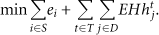
Table 4 shows the results of similar experiments. However, this time the demand points are spread randomly through the sensed area.

Table 4

Simulation results for demand point in aleatory positions.

	Hybrid methodology	Hybrid methodology
Time intervals	6	10
Demand points	400	400
Sensor nodes	36	36
Sinks	1	1
Time (minutes)	146.77 ± 32.45	366.28 ± 13.54
Time for first final solution	91.55 ± 47.14	196.05 ± 78.30
Uncovered demand points (%)	1.56 ± 0.61	2.10 ± 0.53
Real objective	20,472.51 ± 4,135.35	32,522.51 ± 2,628.33

The real purpose of this model is to extend the WSN lifetime as far as possible, preserving the WSN cost. So, lower electrical charge consumption is not necessarily an important issue if it does not reflect in more time slots. The number of time slots multiplied by the duration of each time slot represents this WSN lifetime.

Given this explanation it is reasonable to say that both solutions found by hybrid methodology (HM) and integer linear programming are equivalent in effectiveness. However, the HM approach can handle an amount of sensors 325% times larger, extending the working range of this application.

The only drawback here is the uncovered demand point rate, which is worse than ILP value. Despite this small imperfection of 2.35%, many real applications tolerate some lack of coverage by the nature of the observed phenomenon and other aspects. However, these uncovered demand points are often situated at the periphery of the observed area. The coverage radius does not reflect necessarily a sharp threshold of sensing.

Figure 3 shows the evolution of the best individual fitness in plain line and population fitness average in line with points as well.

Figure 3

Best individual and population average evolution.

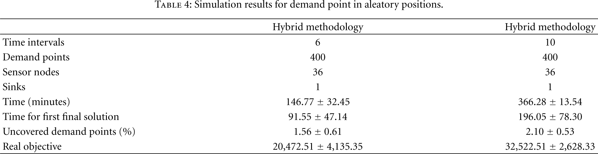
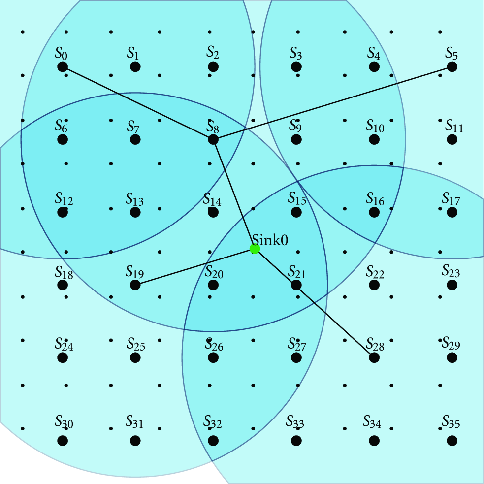
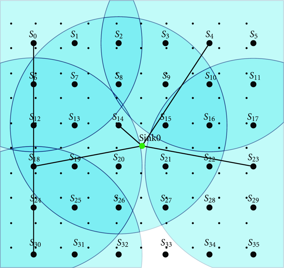
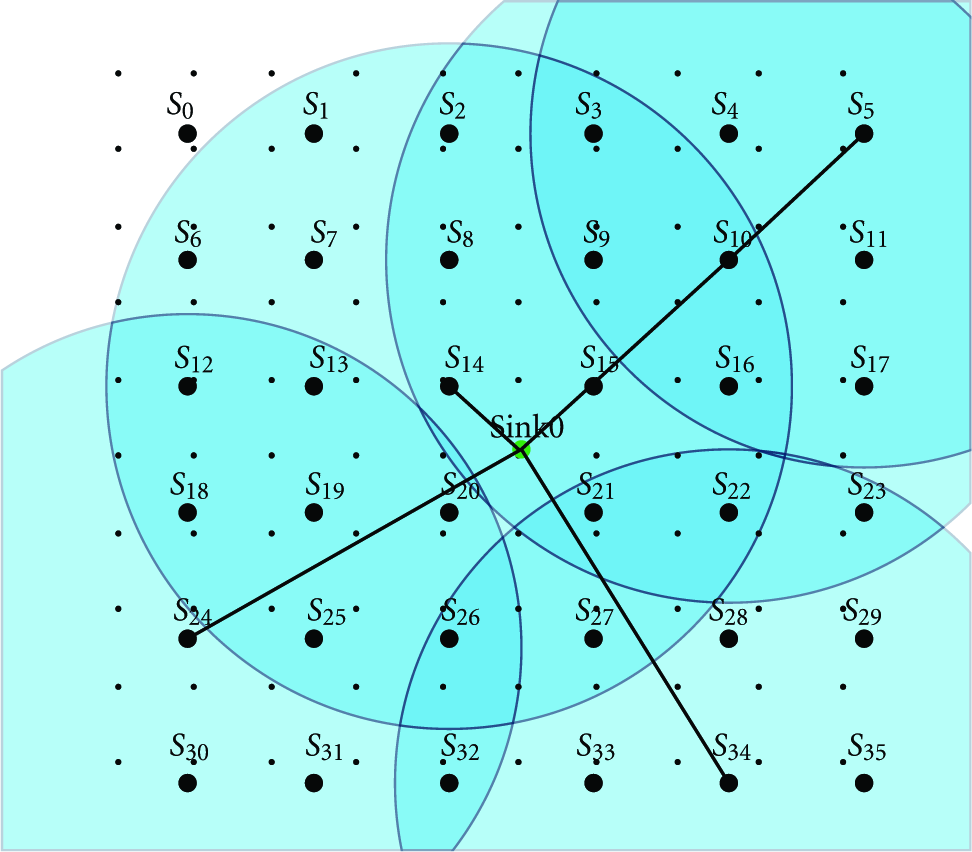
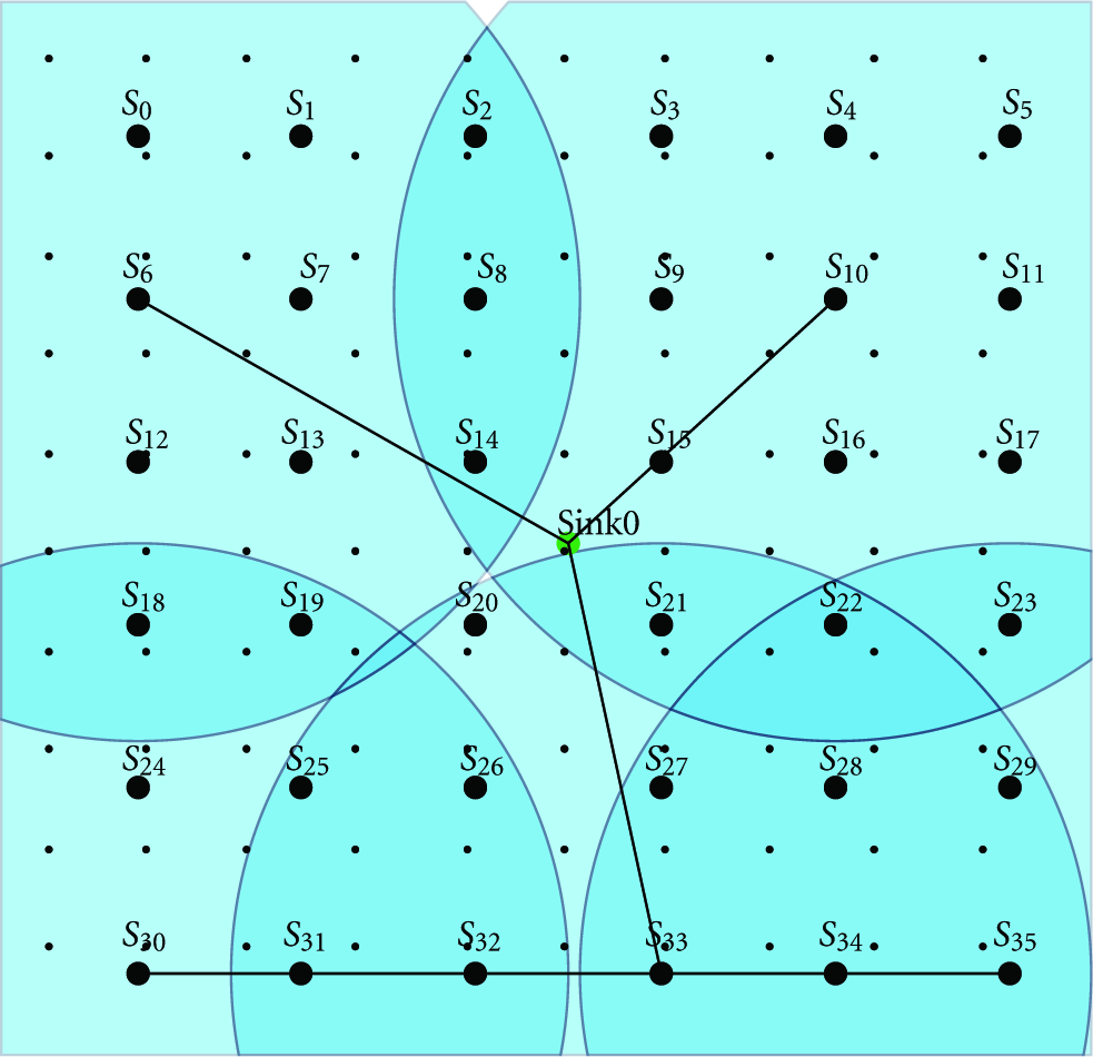
Figures 4, 5, 6, 7, 8, 9, 10, 11, 12, and 13 are graphical representations of 10 time slots of a solution example. It shows the active sensor nodes, their coverage radii, the covered and uncovered demand points, and the routes from sensor nodes to the sink in the center.

Figure 4

Figure 5

Figure 6

Figure 7

Figure 8

Figure 9

Figure 10

Figure 11

Figure 12

Figure 13

7. Conclusion and Future Works

This hybrid methodology is not only suitable for solving complex instances in the domain of cutting and packing problems, but also can be adapted to tackle other problem classes like WSN as shown here. The key point in this adaptation is finding the best or at least a good reducible structure. This analysis is very linked to the chromosome encoding choice as it represents a tradeoff between subproblem complexity range width and chromosome size. A good reducible structure allows a wide range of subproblem complexity from very light and fast subproblems to the actual real problem. On the other hand, the reducible matrix size affects the chromosome size and a large chromosome size reduces the GA effectiveness.

In this problem, a good reducible structure was found, but it is much larger than the ones found in the cutting and packing problem instance. That is the reason why a new chromosome encoding was developed. This new encoding makes the matrix choice viable. The use of integer linear programming approach is limited to a certain level of complexity that sometimes is not enough for a real size network (Table 3).

The results found are far better than reference literature and leave opportunities of future enhancements as new supplementary algorithms and heuristics aggregated to this methodology. In [32] is implemented a hybrid methodology using genetic algorithm to deal with dynamic coverage and connectivity heterogeneous wireless sensor network. The difference between the homogeneous, addressed in this paper, and the heterogeneous, is the last one that has the capacity to deal with different phenomena independently, giving different sample data and sensed range for each phenomenon. This implies in a different way to treat the network's transmission data. Although it does not implement any density explosion control, good solutions are found in feasible execution time for wireless sensor network that could not be possible if only ILP was applied.

Another promising line of investigation involves the design and implementation of parallel/distributed versions of the framework, by means of which several GRIs (generator of reduced instances) and SRIs (solver of reduced instances) instances could run concurrently, each one configured to explore different aspects of the optimization problem at hand. The use of insular GA can bring more diversity and possibilities, resulting in effectiveness enhancement. Also, other metaheuristics such as particle swarm could be experimented replacing or working cooperatively with GA.

Footnotes

Abbreviations

Acknowledgments

The first and second authors are thankful to National Counsel of Technological and Scientific Development (CNPq) via Grants no. 305844/2011-3 and no. 312934/2009-2, the third author is thankful to Coordination for the Improvement of Higher Education Personnel (CAPES), and the fourth author is thankful to Foundation for Support of Scientific and Technological Development Ceara State (FUNCAP) for the support received for this project. The authors also acknowledge IBM for making the IBM ILOG CPLEX Optimization Studio available to the academic community.

References

de Aguiar

A. B.

de Meneses Sobreira Neto

Cunha

R. P. P.

Pinheiro

P. R.

Coelho

A. L. V.

A hybrid methodology for coverage and connectivity in wireless sensor network dynamic planning

Proceedings of the 41st Simpósio Brasileiro de Pesquisa Operacional

2010

Bento Gonçalves, Brazil

Wang

Xing

Zhang

Pless

Gill

Integrated coverage and connectivity configuration in wireless sensor networks

Proceedings of the 1st International Conference on Embedded Networked Sensor Systems (SenSys '03)

November 2003

28 39

2-s2.0-18844371448

Pinheiro

P. R.

Coelho

A. L. V.

Aguiar

A. B.

Neto

A. M. S.

Applying the generate and solve methodology in the problem of dynamic coverage and connectivity in wireless sensor networks

Proceedings of the Information Science and Industrial Applications (ISI) (SERSC '12)

2012

Cebu, Philippines

252 257

Zhou

Liang

Xie

Multiobjective coverage control strategy for energy-efficient wireless sensor networks

International Journal of Distributed Sensor Networks 2012 2012 10

10.1155/2012/720734

720734

Quintão

F. P.

Nakamura

F. G.

Mateus

G. R.

Evolutionary algorithm for the dynamic coverage problem applied to wireless sensor networks design

Proceedings of the IEEE Congress on Evolutionary Computation (IEEE CEC '05)

September 2005

1589 1596

2-s2.0-27144530235

Ishebabi

Mahr

Bobda

Gebser

Schaub

Answer set versus integer linear programming for automatic synthesis of multiprocessor systems from real-time parallel programs

International Journal of Reconfigurable Computing 2009 2009 11

10.1155/2009/863630

863630

Nguyen

Cheung

S. C.

On reducing communication energy using cross-sensor coding technique

International Journal of Distributed Sensor Networks 2011 2011 12

2-s2.0-79955034759

10.1155/2011/837128

837128

Megerian

Koushanfar

Veltri

Potkonjak

Exposure in wireless sensor networks: theory and practical solutions

Wireless Networks 2002 8 5 443 454

2-s2.0-0036738161

10.1023/A:1016586011473

Megerian

Potkonjak

Lower power 0/1 coverage and scheduling techniques in sensor networks

2003 030001

Los Angeles, Calif, USA

University of California

10.

Martins

F. V. C.

Nakamura

F. G.

Quintão

F. P.

Mateus

G. R.

Model and algorithms for the density, coverage and connectivity control problem in flat WSNs

Proceedings of the International Network Optimization Conference

2007

11.

Nakamura

F. G.

Mateus

G. R.

Planejamento dinâmico para controle de cobertura e conectividade em redes de sensores sem fio

Proceedings of the Workshop de Comunicação sem Fio e Computação Móvel

2004

182 191

12.

de Aguiar

A. B.

Pinheiro

P. R.

Coelho

A. L. V.

Optimizing energy consumption in heterogeneous wireless sensor networks: a novel integer programming model

Proceedings of the 4th International Conference on Operational Research for Development (ICORD '07)

2007

496 505

13.

de Aguiar

A. B.

Pinheiro

P. R.

Coelho

A. L. V.

Neto

A. S.

Cunha

R. P. P.

Scalability analysis of a novel integer programming model to deal with energy consumption in heterogeneous wireless sensor networks

Communications in Computer and Information Science 2008 14 11 20

14.

Aguiar

A. B.

Tackling the problem of dynamic coverage and connectivity in wireless sensor networks with an extended version of the generate and solve methodology generate and solve methodology [M.S. dissertation] 2009

Graduate Program in Applied Informatics, University of Fortaleza

15.

Blum

Roli

Metaheuristics in combinatorial optimization: overview and conceptual comparison

ACM Computing Surveys 2003 35 3 268 308

2-s2.0-0344236266

10.1145/937503.937505

16.

Dumitrescu

Stützle

Combinations of local search and exact algorithms

Lecture Notes in Computer Science 2003 2611 211 223

2-s2.0-35248813358

17.

Talbi

E. G.

A taxonomy of hybrid metaheuristics

Journal of Heuristics 2002 8 5 541 564

2-s2.0-0036723306

10.1023/A:1016540724870

18.

Pinheiro

P. R.

Coelho

A. L. V.

de Aguiar

A. B.

Bonates

T. O.

On the concept of density control and its application to a hybrid optimization framework: investigation into cutting problems

Computers and Industrial Engineering 2011 61 463 472

2-s2.0-79955566544

10.1016/j.cie.2011.03.013

19.

Nepomuceno

N. V.

Pinheiro

P. R.

Coelho

A. L. V.

Tackling the container loading problem: a hybrid approach based on integer linear programming and genetic algorithms

4446

Proceedings of the EvoCOP

2007

Valência, Spain

Springer

154 165 Lecture Notes in Computer Science

20.

Nepomuceno

Pinheiro

Coelho

A. L. V.

A hybrid optimization framework for cutting and packing problems: case study on constrained 2D non-guillotine cutting

Studies in Computational Intelligence 2008 153 87 99

2-s2.0-51649094333

10.1007/978-3-540-70807-0_6

21.

Araújo

L. J. P.

Pinheiro

P. R.

Combining heuristics backtracking and genetic algorithm to solve the container loading problerm with weight distribution

Advances in Intelligent and Soft Computing 2010 73 95 102

22.

de Araujo

L. J. P.

Pinheiro

P. R.

Applying backtracking heuristics for constrained two-dimensional guillotine cutting problems

Lecture Notes in Computer Science 2011 7030 113 120

23.

Bhondekar

A. P.

Vig

Singla

M. L.

Ghanshyam

Kapur

Genetic algorithm based node placement methodology for wireless sensor networks

Proceedings of the International MultiConference of Engineers and Computer Scientists (IMECS '09)

2009

Hong Kong

18 20

24.

Eiben

A. E.

Smith

J. E.

Introduction to Evolutionary Computing 2003

Springer

25.

Back

Fogel

D. B.

Michalewicz

Handbook of Evolutionary Computation 1997

Bristol, UK

IOP

26.

Wolsey

L. A.

Integer Programming 1998

John Wiley & Sons

27.

Puchinger

Raidl

G. R.

Combining metaheuristics and exact algorithms in combinatorial optimization: a survey and classification

3562

Proceedings of the 1st International Work Conference on the Interplay between Natural and Artificial Computation (IWINAC '05)

June 2005

41 53 Lecture Notes in Computer Science

2-s2.0-26444552169

28.

de Aguiar

A. B.

Neto

A. d. M. S.

Pinheiro

P. R.

Coelho

A. L. V.

Applicability of a novel integer programming model for wireless sensor networks

International Journal of Computer Science and Information Security 2009 20093 1 7 13

29.

ILOG. ILOG CPLEX 10.0 User's Manual. United States of America, January 2006

30.

De Andrade

I. B. D.

Mateus

G. R.

Nakamura

F. G.

A GRASP heuristic to density control: solving multi-period coverage and routing problems in wireless sensor networks

Proceedings of the 14th IEEE Symposium on Computers and Communications (ISCC '09)

July 2009

Sousse, Tunisia

493 499

2-s2.0-70449507257

10.1109/ISCC.2009.5202370

31.

Quintão

F. P.

Nakamura

F. G.

Mateus

G. R.

A hybrid approach to solve the coverage and connectivity problem in wireless sensor networks

Proceedings of the 4th European Workshop on Metaheuristics: Design and Evaluation of Advanced Hybrid Metaheuristics

2004

Nottingham, UK

32.

Neto

A. M. S.

Um modelo em otimização de energia aplicado às redes de sensores sem fio heterogêneas

Graduation Conclusion Work, Graduate in Computer Science, University of Fortaleza, 2010

Towards Aid by Generate and Solve Methodology: Application in the Problem of Coverage and Connectivity in Wireless Sensor Networks

Abstract

1. Introduction

2. The Wireless Sensor Network

3. Model

4. The Base Hybrid Methodology

5. Improvements for the Dynamic Coverage and Connectivity in Wireless Sensor Network Problem

5.1. Spread Sensor Heuristic in Population Initialization

5.2. Compact Chromosome Encoding

6. Computational Results

7. Conclusion and Future Works

Footnotes

Abbreviations

Acknowledgments

References